This document describes sequence-to-sequence (seq2seq) models, including an overview of encoder-decoder architectures using recurrent neural networks. It explains how seq2seq models can be used for applications like machine translation, question answering, and summarization. Attention mechanisms are introduced to allow the decoder to focus on different parts of the input sequence at each time step. Variational seq2seq models with variational attention are also described, where the context vector is modeled as a random variable to avoid bypassing the latent code. The document provides examples and results on question generation and dialogue tasks.

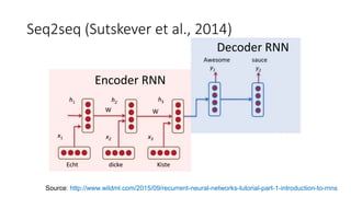
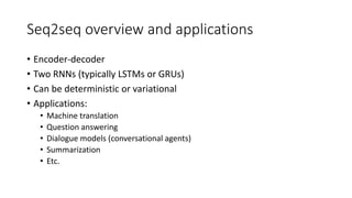
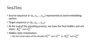
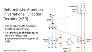
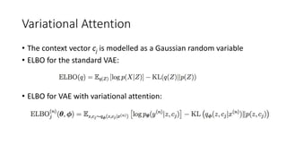
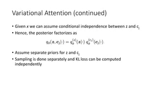
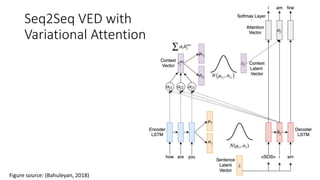
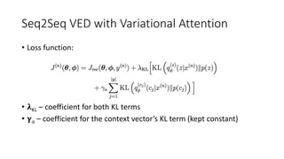
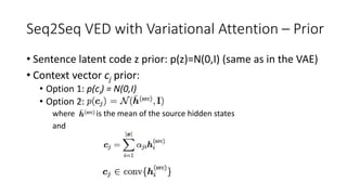
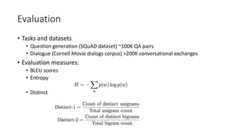
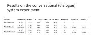
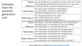
1. 27 Jan 2016
Sequence-to-sequence models

2. Seq2seq (Sutskever et al., 2014)
Source: http://www.wildml.com/2015/09/recurrent-neural-networks-tutorial-part-1-introduction-to-rnns
Encoder RNN
Decoder RNN

3. Seq2seq overview and applications
• Encoder-decoder
• Two RNNs (typically LSTMs or GRUs)
• Can be deterministic or variational
• Applications:
• Machine translation
• Question answering
• Dialogue models (conversational agents)
• Summarization
• Etc.

4. LSTM cell

5. Seq2Seq
• Source sequence x= (x1, x2,..., x|x|) represented as word embedding
vectors
• Target sequence y= (y1, y2,..., y|y|)
• At the end of the encoding process, we have the final hidden and cell
states
• Hidden state initialization:
• Set the initial states of the decoder to

6. Seq2seq (cont.)
• At each step of the decoder, compute
• yj-1 – ground truth previous word during training (“teacher forcing”),
and previously predicted word at inference time.
• θ – parameters (weights) of the network

7. Seq2seq (cont.)
• Predicted word at time step j is given by a softmax layer:
• Wout is a weight matrix
• Softmax function:
• yjk is the value of the kth dimension of the output vector at time step j

8. Softmax example
Source: (Bahuleyan, 2018)

9. Seq2seq model
Source: (Bahuleyan, 2018)

10. Selecting the word at each time step of the
decoder
• Greedy search: select word with the highest p(yi) given by the
softmax layer
• Beam search: choose k words with the highest p(yi) at each time step.
• k – beam width (typically 5-10)

11. Beam search
• Multiple possible replies
can be generated in
response to “Who does
John like?”
Image source: https://www.analyticsvidhya.com/blog/2018/03/essentials-of-deep-learning-sequence-to-sequence-modelling-with-attention-part-i/

12. Beam search (cont.)
Image source: https://www.analyticsvidhya.com/blog/2018/03/essentials-of-deep-learning-sequence-to-sequence-modelling-with-attention-part-i/
• Chose the proposed path
with the maximum
combined probability

13. Seq2seq resources
• https://blog.keras.io/a-ten-minute-introduction-to-sequence-to-
sequence-learning-in-keras.html

14. Attention mechanism in RNN encoder-
decoder networks – Intuitions
• Dynamically align target sequence with source sequence in the
decoder
• Pay different level of attention to words in the input sequence at each
time step in the decoder
• At each time step, the decoder is provided access to all encoded
source tokens
• The decoder gives higher weights to certain and lower to others

15. Attention mechanism – Formal definition
• Compute a probabilistic distribution at each decoding time step j
where is the weight given to source output i and
is a pre-normalized score

16. • Two methods to compute :
• Multiplicative (Luong et al., 2015)
• Additive (Bahdanau et al., 2014)
Attention mechanism – Formal definition (cont.)

17. • Take the sum of the source outputs weighted by to get
the context vector
• Compute attention vector
• Finally, feed attention vector to the softmax layer
Attention mechanism – Formal definition (cont.)

18. Seq2seq model
with attention
Figure source: (Bahuleyan, 2018)

19. Visualizing Attention in Machine Translation (1)
Source: https://aws.amazon.com/blogs/machine-learning/train-neural-machine-translation-models-with-sockeye/

20. Visualizing Attention in Machine Translation (2)
Source: https://aws.amazon.com/blogs/machine-learning/train-neural-machine-translation-models-with-sockeye/

21. Variational Attention for
Sequence-to-Sequence Models
Hareesh Bahuleyan, Lili Mou, Olga Vechtomova, Pascal Poupart
In Proc. COLING 2018

22. Figure source: (Bahuleyan, 2018)
• The decoder LSTM has direct
access to source via cj
• This may cause the decoder to
ignore z – bypassing
phenomenon (Bahuleyan et al.,
2018)
Deterministic Attention
in Variational Encoder-
Decoder (VED)

23. Variational Attention
• The context vector cj is modelled as a Gaussian random variable
• ELBO for the standard VAE:
• ELBO for VAE with variational attention:

24. Variational Attention (continued)
• Given x we can assume conditional independence between z and cj
• Hence, the posterior factorizes as
• Assume separate priors for z and cj
• Sampling is done separately and KL loss can be computed
independently

25. Seq2Seq VED with
Variational Attention
Figure source: (Bahuleyan, 2018)

26. Seq2Seq VED with Variational Attention
• Loss function:
• 𝛌KL – coefficient for both KL terms
• 𝛄𝑎 – coefficient for the context vector’s KL term (kept constant)

27. Seq2Seq VED with Variational Attention – Prior
• Sentence latent code z prior: p(z)=N(0,I) (same as in the VAE)
• Context vector cj prior:
• Option 1: p(cj) = N(0,I)
• Option 2:
where is the mean of the source hidden states
and

28. Seq2Seq VED with Variational Attention –
Posterior
• Both posterior distributions q(z|x) and q(cj|x) are
parameterized by the encoder LSTM
• For the sentence latent space (same as VAE):
• For the context vector cj at time step j:
Where , and is computed using feed-forward neural
network

29. Evaluation
• Tasks and datasets
• Question generation (SQuAD dataset) ~100K QA pairs
• Dialogue (Cornell Movie dialogs corpus) >200K conversational exchanges
• Evaluation measures:
• BLEU scores
• Entropy
• Distinct

30. Results on the question generation task
Source: Bahuleyan et al (2018) https://arxiv.org/abs/1712.08207

31. Results on the conversational (dialogue)
system experiment

32. Examples
from the
question
generation
task
Source: Bahuleyan et al (2018) https://arxiv.org/abs/1712.08207