Effects oftheExchange Interaction Parameter onthePhase Diagrams fortheTransverse Ising Model

Bayor Jude Simons et al Int. Journal of Engineering Research and Applications www.ijera.com
ISSN : 2248-9622, Vol. 5, Issue 1( Part 2), January 2015, pp.127-131
www.ijera.com 127|P a g e
Effects oftheExchange Interaction Parameter onthePhase
Diagrams fortheTransverse Ising Model
Bayor Jude Simons*, BaohuaTeng**, Manoj Kumar Shah***
*(School of Physical Electronics, University of Electronic Science and Technology of China, Chengdu
610054,P.R. China)
**(School of Physical Electronics, University of Electronic Science and Technology of China, Chengdu
610054,P.R. China)
*** (School of Optoelectronic Information, University of Electronic Science and Technology of China,
Chengdu 610054,P.R. China)
ABSTRACT
The microscopic effect of the exchange interaction parameter for the 2-Dimensional ising model with nearest
neighbor interaction has been studied. By supposing simple temperature dependent relationship for the exchange
parameter, graphs were straightforwardly obtained that show the reentrant closed looped phase diagrams
symptomatic of some colloids and complex fluids and some binary liquids mixtures in particular. By parameter
modifications, other phase diagrams were also obtained. Amongst which are the u-shapes and other exotic
shapes of phase diagrams. Our results show that the exchange interaction parameter greatly influence the size of
the ordered phase. Hence the larger the value of the constant, the larger the size of the ordered phase. This means
that the higher values of the exchange parameter brings about phase transitions that straddle a wider range of
polarizations and temperatures.
Keywords-closed loop, exchange interaction, order-disorder, phase diagram, reentrant behavior, transverse Ising
model (TIM).
I. Introduction
Phase diagrams can allow us to obtain a deeper
understanding of some intriguing states of matter
especially how various systems make transitions
between the different states of matter. Hence while
experimentally obtained phase diagrams have been
helpful in the onset, they have not been tractable in
disposition. The interest in phase diagrams lies in
how the size and shapes of the closed loops varied
with various parameters [1]. Thus with the aid of
mathematical models, calculations of phase diagrams
have enhanced the understanding of the underlying
microscopic physical property changes that takes
place within physic-chemical systems. Hence the
shapes of various phase diagrams have been obtained
by various models and simulations [2-27]. Teng et al
[27] investigated the phase diagram for a ferroelectric
thin film described by the TIM with four spin
interaction. Campi et al [25] studied Ising model with
temperature dependent interactions and reports that
the model can generate various phase diagrams, and
some having shapes as those of complex fluids.
Indeed the most intriguing aspect of phase
transition phenomena is the reentrant behavior of
some complex fluids and physico-chemical systems.
Reentrant phase behavior offers a lot more insight
into the microscopic behavior of atoms and
molecules of matter. Recently the studies of
reentrant behavior has gained the attention of some
researchers. Redner et al [28] studied the reentrant
phase behavior in active colloids with attraction. The
reentrant liquid-liquid phase separation in protein
solutions at elevated hydrostatic pressures was
investigated by Moller et al [29]. The observation of
a reentrant phase transition in incommensurate
potassium was studied by Lundegaard et al [30].
While Kaneyoshi et al studied reentrant phenomena
in a transverse Ising nanowire (or nanotube) with a
diluted surface: Effects of interlayer coupling at the
surface [31].
At this point it will be pertinent to explain the
reentrants behaviors as exhibited by complex fluids
especially in some binary liquids. This is because
binary liquids were the medium in which were first
discovered. Hence some binary mixtures of fluids
show this characteristic reentrant property of
reappearing phases. Thus a graph their temperature
versus concentration phase diagram are closed-
looped curves [32]. Earlier on the considerations of
energy effects alone was not sufficient to explain the
reasons why binary fluids become miscible at high
temperatures. The answer to this was found in the
concept of entropy. Hence a mixtures becomes
miscible at high temperatures because the system
tends not to minimize its energy but rather its
free energy. For a system at a low temperature,
entropy changes will not make much difference in
its free energy. At high temperatures, on the other
RESEARCH ARTICLE OPEN ACCESS

hand, changing the entropy by even a small
amount has a large effect on the free energy, and
so at high temperatures systems tend to maximize
their entropy and in so doing becomes disordered.
However the question remained unanswered how
the system becomes disordered again at low
temperatures, since entropy influence decreases with
decreasing temperature. As temperature is lowered,
energy tends to dominate. Hence gradually the
lowered energy becomes associated with the van
der Waals attraction which has a larger effect on
the free energy than the entropy does. The mixture
then becomes immiscible since there are grouping of
like molecules. Further lowering of the mixture's
temperature brings about the immiscible phase. At
sufficiently low temperature, then the low energy of
hydrogen bonding tend to have a greater effect on the
system’s free energy. At below this point the mixture
becomes miscible again. This mixture has the same
macroscopic properties as the high-temperature
miscible mixture [33].
Various models of this system have been studied.
Using the mean-field approximation approach,
Barker and Fock [34] obtained closed-looped phase
diagrams with the model. However there was a
difference between the observed coexistence phases
and the concentration by comparison with
experiment. Then, Wheeler [35] Andersen [36]
presented the model called the decorated lattice-gas.
This also produced closed-loop phase. In comparison
with the treatment by the Ising model. It doesn’t deal
well with the interactions amongst the nearest
neighbor molecules at each lattice as the Ising model
does.
In this paper, we investigate the microscopic
properties of TIM with temperature dependent
potential parameters. Of particular focus is how the
exchange interaction parameter affects the shapes of
various phase diagrams that all commonly originate
from the closed loop phase diagrams of binary fluids
by parameter modification.
II. The Model
We consider the transverse Ising model with
nearest neighbor interaction only, since it has proved
to be efficient in the calculation of phase diagram of
complex fluids [17-20, 37] with reentrant phase
behavior. Its Hamiltonian is given as follows [17-20,
37]:
,
x z z
i i j
i i j
H S JS S    
(1)
where x
iS and z
iS are the x- and z-components of a
pseudospin-1/2 operator at site i in the lattice, and
ji,
runs over only distinct nearest-neighboring
pairs. Ω is the transverse field and J is the
exchange interaction constant between nearest
neighbor spins.
Within the framework of the mean-field theory, the z
component of the pseudospin can be written as
(2)
where and .In fact,
the ensemble average of the pseudo-spin is
understood as the order parameter of the system
(subsequently, we use SS in place of in
labelling the graphs).Here the order parameter of the
system is the ensemble average of the pseudo-spin
z
iS , and describes the transition of the system from
order (
z
iS ≠0) to disorder (
z
iS =0) state [37].
Experimental research in complex fluids has
established that temperature changes in systems may
have a direct correlation with the exchange
interaction parameter [10-11], while for some crystal
materials the exchange parameter shows positive
relationship with temperature.
With the ising model concept of an effective
exchange interaction and the correlative temperature
dependence was used by Campi and Krivine [25] to
obtain closed-loop shaped phase diagrams and
described the reentrant phase behavior of complex
fluids. Therefore Simons et al using transverse Ising
model and supposing that the effective exchange and
effective transverse field parameters J and 
developed the simple temperature-dependent
relations as follows [37]:
0
0
n
T
J J
T
 
  
 
and
0
0
m
T
T
 
    
 
(3)
where 0T are arbitrary constant. Here the effective
parameters 0J , 0 and Bk T are reduced by 0Bk T ,
and simply are notated still as 0J , 0 and t. By this
therefore, we can calculate the phase diagram on the
polarization-effective temperature space with
effective temperature-dependent exchange interaction
parameters.
III. The Phase diagrams
In this section we obtain the phase diagrams in
polarization-temperature space. Graphs are plotted
with the polarizations for various parameters of (J0, n,
Ω0 and m) vrs the effective temperature t. By varying
the effective exchange parameter J0, we can observe
the effect it has on the phase transition diagram.
In fig.1, we see the effect of changing the
effective exchange parameter (J0) while keeping all
other parameters constant. The plots are closed
looped curves that are symmetrical along the
   0 02 tanh 2z
i BS k T  
2 2 2
0    z
i
i
J S  
z
iS
z
iS

horizontal axis and shows typical phase diagrams for
reentrant phase behavior. Thus at very low
temperatures, the system is in disordered state, while
at intermediate temperatures it is in the ordered state
then at high temperatures it is again in the disordered
state. When J0 is high (J0= 1.6), the closed looped
curves are broader and covers a wider spectrum of
concentration and temperature. This means the region
for which the system is ordered is bigger. As J0
decreases to 1.05, the closed loop profiles also
progressively decrease, and as a result the ordered
region diminishes while the disordered region
becomes more dominant.
Fig.1. Phase transition diagram showing the
polarization ss for various J0 parameters given n=1.5.,
Ω0=1.1 and m=2.2 vs temperature t.
Fig. 2 shows a system with mixed fortunes when
it comes to the property of reentrant behavior. First of
all for this system, when J0 is large, the system has
only two transition states, and is ordered at low
temperatures and disordered at high temperatures.
But when J0 is small, then the reentrant phase
property appears similar to fig. 1 above. Hence the
system is disordered at high temperatures, ordered at
intermediate temperatures and again becomes
disordered at low temperatures. For these systems,
the bigger the J0 values, the bigger the ordered phase.
Fig. 2Phase transition diagram showing the
polarization ss for various J0parameters given n=1.2,
Ω0=1.1 and m=2.2 against temperature t.
Fig. 3 shows the category of phase diagrams
which have the U-shape profiles. The phase profiles
are concentric half circles and these systems exhibit
the normal sequence of phase transitions with
temperature. Hence at low temperatures the system is
ordered and at high temperatures it is disordered. The
smaller the value of J0 becomes, the smaller the
region of the ordered phase. This means that the
range of polarization and temperature for the ordered
phase gets smaller while that of the disordered phase
gets larger. This phase diagram is synonymous with
ferromagnetic-paramagnetic phase transition systems.
Fig. 3. Phase transition diagram showing the
polarization ss for various J0parameters given n=1.0,
Ω0=1.1 and m=2.2 against temperature t.
The fourth category of phase behavior can be
found in fig. 4. Here at temperature t=0, all the
various systems are equally polarized. The phase
profiles are crescent-shaped half circles. This
therefore means that they have two distinct phase

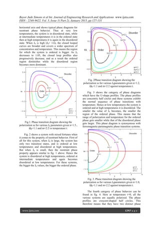
states. At low temperatures, the system is at the
ordered state and at high temperatures it is in the
disordered state. As J0 decreases from 2.5 to 1.1, the
region for the ordered phase also decreases and as a
result only the temperature range for the ordered
phase decreases.
Figure 4. Phase transition diagram showing the
polarization ss for various J0parameters givenn=0.6,
Ω0=1.1 and m=2.2) against temperature t
IV. Conclusions
This paper studies the effect of the exchange
interaction parameter J0 on the mathematical
framework of the ising model with temperature
dependent relations. Graphical plots were obtained
by theoretical formulations from the model using the
Mathcad software. First of all the graphs obtained
were categorized according to the various shapes of
phase diagrams that have been observed for systems
both theoretically and experimentally.
By obtaining the more complex phase diagram
of the reentrant closed loop phase behavior in the first
category, other phase diagrams were obtained by
parameter modifications of the first category systems.
Other exotic shapes such as U shape and the D-shape
and crescent-shaped were obtained and analyzed.
Our results basically show that systems become
more disordered when the exchange interaction
parameter is decreased. As a result, the ordered phase
ranges of polarization and temperatures diminishes
with a decrease in the exchange interaction parameter
influence.
References.
Journal Papers:
[1] J. S. Walker and C. A. Vause. Phys. Lett.
A, 79 (1980) 421.
[2] K. Murata and H. Tanaka. Nature Mater, 11
(2012) 436.
[3] R. Dong and J. C. Hao. Chem. Rev., 110
(2010) 4978.
[4] J. Liu, H. Gomez, J. A. Evans, T. J. R.
Hughes and C. M. Landis. J. Comput. Phys.,
248 (2013) 47.
[5] M. Laurati, C.M.C. Gambi, R. Giordano, P.
Baglioni, and J. Teixeira. J. Phys. Chem. B,
114 (2010) 3855.
[6] A. Reinhardt, A. J. Williamson, J. P. K.
Doye, J. Carrete, L. M. Varela, and A. A.
Louis. J. Chem. Phys., 134 (2011) 104905.
[7] N. S. A. Davies and R. D.Gillard. Trans.
Met. Chem., 25 (2000) 628.
[8] J. S. Walker and C. A. Vause. Reappearing
Phases, Sci. Am., May issue (1987) 90.
[9] S. Moelbert and P. De Los Rios.
Macromolecules, 36 (2003) 5845.
[10] S. H. Chen, J. Rouch, F. Sciortino, and P.
Tartaglia Chen. J. Phys.: Condens. Matter, 6
(1994) 10855.
[11] L. A. Davies, G. Jackson, and L. F. Rull.
Phys. Rev. Lett., 82 (1999) 5285.
[12] C. S. Hudson. Z. Phys. Chem., 47 (1904)
113
[13] J. C. Lang and R. D. Morgan. J. Chem.
Phys., 73 (1980) 5849.
[14] F. F. Nord, M. Bier, and S. N. Timasheff. J.
Am. Chem. Soc., 73 (1951) 289.
[15] T. Narayanan and A. Kumar. Phys. Rep.,
249 (1994) 135-218.
[16] C. L. Dias. Phys. Rev. Lett., 109 (2012)
048104.
[17] C. L. Wang, W. L. Zhong, and P. L. Zhang.
J. Phys.: Condens. Matter, 3 (1992) 4743.
[18] T. Kaneyoshi. Physica A, 293 (2001) 200
[19] J. M. Wesselinowa. Solid State Comm., 121
(2002) 489.
[20] A. Saber, S. Lo Russo, G. Mattei, and A
Mattoni. JMMM, 251 (2002) 129
[21] B. H. Teng and H. K. Sy. Phys. Rev. B, 70
(2004) 104115
[22]
[23] A. Badasyan, S. Tonoyan, A. Giacometti, R.
Podgornik, V. A. Parsegian, Y.
Mamasakhlisov and V. Morozov. Phys. Rev.
Lett., 109 (2012) 068101.
[24] M. Zamparo and A. Pelizzola. Phys. Rev.
Lett., 97 (2006) 068106.
[25] X. Campi and H. Krivine. Europhys. Lett.,
66 (4) (2004) 527.
[26] C. N. Likos. Phys. Rep., 348 (2001) 267.
[27] B. H. Teng and H. K. Sy. Europhys. Lett.,
73 (4). 2006. Pp 601-606
[28] G. S. Redner, A. Baskaran, and M. F.
Hagan. Physical Review E88, 012305 (2013)
[29] J. Möller, S. Grobelny, J. Schulze,S. Bieder,
A. Steffen, M. Erlkamp, M. Paulus,
M.Tolan, and R. Winter.Phys. Rev. Lett.,
112 (2014) 028101

[30] L. F. Lundegaard, G. W. Stinton, M.
Zelazny, C. L. Guillaume, J. E. Proctor, I.
Loa, E. Gregoryanz, R. J. Nelmes, and M. I.
McMahon. Physical Review B88, 054106
(2013)
[31] T. Kaneyoshi. Journal of Magnetism and
Magnetic Materials 339 (2013) 151–156
[32] A. Kumar, S. Guha and E.S.R. Gopal.
Physics Letters Volume 123, no. 9A (1987)
[33] B.C. McEwan, 3. Chem. Soc. 123 (1923)
2284.
[34] J.A. Barker and W. Fock, Discuss. Faraday
Soc. 15 (1953) 188.
[35] J.C. Wheeler, 3. Chem. Phys. 62 (1975) 433.
[36] G.R. Andersen and J.C. Wheeler, J. Chem.
Phys. 69 (1978) 2082.
[37] B. J. Simons, B. H. Teng, S. Zhou, L. Zhou,
X. Chen, M. Wu and H. Fu. Chem. Phys.
Lett., 605–606 (2014) 121
Books:
[22] D. Poland and H. A. Scheraga. Theory of
helix-coil transitions in biopolymers(New
York: Academic Press 1970)

Effects oftheExchange Interaction Parameter onthePhase Diagrams fortheTransverse Ising Model

More Related Content

What's hot

Viewers also liked

Similar to Effects oftheExchange Interaction Parameter onthePhase Diagrams fortheTransverse Ising Model

Recently uploaded

Effects oftheExchange Interaction Parameter onthePhase Diagrams fortheTransverse Ising Model