Using Spreadsheets.pptx

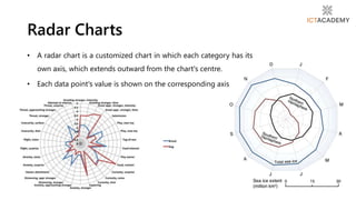
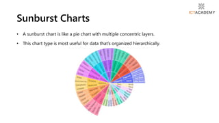
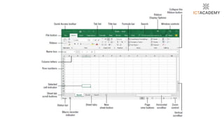
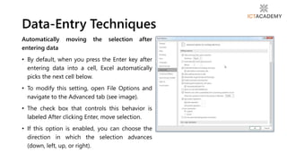
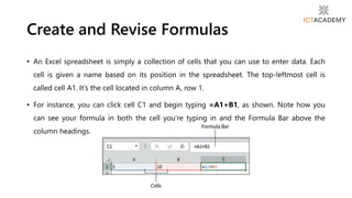
• The Excel worksheet is an electronic ledger created by the Microsoft Excel spreadsheet
program
• Excel has series of rows and columns separated into cells.
• Users can store and manipulate data in rows and columns divided by cells using
worksheets.
• Worksheets frequently enable users to easily write equations and logical functions to
execute certain worksheet features.
Introduction

Data Features, Formulas and Shortcuts
• Excel has a number of functions, formulae, and shortcuts that can be used to increase the
software's usefulness.
Accounting and Business use
• Excel is a widely used spreadsheet programme in finance and accounting.
• Additionally, numerous businesses conduct all budgeting, forecasting, and accounting
operations solely through Excel spreadsheets.
Introduction

Difference between Tables and Worksheets
• A worksheet contains tens of thousands of rows and columns, and occasionally even a million.
• Tables, on the other hand, are designed to use fewer rows and columns to organize related data for
sorting and filtering purposes.
• Tables also support the inclusion of links to external networks, although worksheets do not.
Formatting Tables
• Tables include many of the same formatting possibilities as spreadsheets, but they also allow users
to import and export data from external networks, display and use more tools in Excel tables, and
even sort and filter information inside the table based on current demand.
Introduction

Importing a Table from External Resources
• There are several ways to import a table from another source. The best approach to do this is to
copy and paste the data from the external resource into your worksheet.
• This form has various flaws. One of the main challenges with copying and pasting is that Excel
doesn't comprehend why you want to build a table.
• This means that after copying and pasting the data into your spreadsheet, you must insert it into a
table in the worksheet
Introduction

Exporting Table to External Resources
• The copy and paste method is similar to importing data, except that you can copy data from your
Excel table and paste it to an external network.
• It allows for more flexibility, but requires a deeper understanding of standard formats and external
resource architectures.
Creation of Excel
• Excel was developed by Microsoft Corporation in 1984.
• This was developed to make data measurement easier for spreadsheet users without using the DOS
command line.
• Until 1992, it was the only spreadsheet programme that required a window.
Introduction

Characteristics of Workbook
• Worksheets offer a variety of functions to Excel users.
• The major role of worksheets is to enable the storage and management of data in a centralized area.
• Nonetheless, with the introduction of spreadsheets, users can now quantify both simple and difficult
mathematical and financial problems, as well as visualize their stored data using any customized
charts and graphs.
• Additionally, Microsoft Excel Tools has developed essential tools and menus that enable Excel users
to customize their Excel programmes and files.
Introduction

Excel uses
• Create budgets, keep track of costs, analyse survey findings, and perform virtually any other type of
financial analysis you may imagine.
• Create a variety of highly customizable charts
• Use the row and column layout to store lists effectively
• Clean up and standardize text-based data
• Import data from variety of sources
• Create graphical dashboards – Summarize a large amount of business information in a concise manner
• Use graphics and diagrams to create professional look
Introduction

Components of MS Excel
Component Functionality or Purpose of the Component
File button
This button opens the Backstage view, which includes a variety of choices for
interacting with your document (including printing) and configuring Excel.
Quick Access
Toolbar
This customizable toolbar provides quick access to frequently used commands.
Regardless of the tab selected, the Quick Access toolbar is always visible.
Tab List Utilize these commands to create a new Ribbon, comparable to a menu.
Title bar
This displays the program's name and the current workbook's name. Additionally, it
contains the Quick Access toolbar (on the left) and a few control buttons for
modifying the window (on the right).
Formula bar This bar displays the information or formulas entered into a cell

Search
The Search control is a magnifying glass with the message "Inform me of your
intent." This control can be used to identify instructions or to have Excel execute
them automatically.
Ribbon Display
options
A drop-down control that offers three options related to displaying the Ribbon.
Window
Controls
These are three controls that are shared by practically all Windows applications for
minimizing the current window, maximizing or restoring the current window, and
shutting the current window.
Collapse the
Ribbon button
To temporarily hide the Ribbon, click this button. To keep the Ribbon visible, double-
click any Ribbon tab. Ctrl+F1 is a shortcut that performs the same function.
Ribbon
This is the primary area where Excel commands are stored. By selecting an item from
the tab list, you can alter the appearance of the Ribbon.

Name box
This box indicates the address of the currently active cell or the name of the
currently selected cell, range, or object.
Column letters
The letters range from A to XFD, one for each of the worksheet's 16,384 columns. You
can choose a complete column by clicking on a column heading, or you can modify
the column width by clicking between the columns.
Row numbers
There are a total of 1,048,576 numbers - one for each row in the worksheet. You can
choose a complete row by clicking on a row number, or you can modify the row
height by clicking between the row numbers.
Selected cell
indicator
To temporarily hide the Ribbon, click this button. To keep the Ribbon visible, double-
click any Ribbon tab. Ctrl+F1 is a shortcut that performs the same function.

Sheet tab scroll
buttons
These buttons allow you to scroll through the sheet tabs and display tabs that are
not visible. Additionally, you can right-click to display a list of sheets.
Status bar
This bar displays numerous messages in addition to the state of your keyboard's Num
Lock, Caps Lock, and Scroll Lock keys. Additionally, it displays summary information
about the specified region of cells. To alter the information displayed in the status bar,
right-click it.
Macro
recorder
Indicator
Click, to begin recording a macro in Visual Basic for Applications (VBA). While your
actions are being recorded, the icon changes. Click once more to pause the
recording.
Sheet tabs
Each of these notebook-style tabs corresponds to a distinct workbook sheet. A
workbook may have an unlimited number of sheets, and each sheet is identified by
its name in a sheet tab.

New Sheet
button
By clicking the New Sheet button, you may create a new worksheet (which is
displayed after the last sheet tab).
Page View
buttons
These buttons allow you to customize the way the worksheet is displayed.
Horizontal
Scrollbar
This tool is used to horizontally scroll the sheet.
Zoom control Use this to zoom your worksheet in and out.
Vertical
Scrollbar
Use this to scroll the sheet vertically.

Protect Workbook
• to password-protect the Excel workbook file, to protect its contents, or to verify the file's contents using a
digital signature
Inspect Workbook
• to look for hidden metadata (file information) and check for accessibility for disabilities and compatibility
with older Excel versions
Manage Workbook
• to recover or delete draught versions of Excel that have been saved using the AutoRecover function
Browser View Options
• to restrict which sections of an Excel workbook may be read and altered by individuals who access it via
the Web
Backstage View

Properties
• displays the file's size as well as any Title, Tags, and Categories set to it (to aid in identifying the file when
performing a search for the workbook)
• to add or modify additional file properties, click the Properties drop-down button and then on the Show
Document Panel or Advanced Properties drop-down option that appears.
Related Dates
• lists the date the file was Last modified, Created and last printed
Related People
• The author of the workbook is listed, as is the person who last edited the file.
Show All Properties Link
• When clicked, the list of Properties is expanded to include editable text boxes for the Comments,
Template, Status, Categories, Subject, Hyperlink Base, and Company.
Backstage View

Ribbon has following components
• Tabs: Excel's primary tasks are consolidated and shown together with all the commands that are often
required to complete that core job.
• Groups: Related command buttons can be grouped together to conduct subtasks that are generally
done as part of the tab's primary task.
Ribbon

Ribbon has following components
• Command button: Each group has command buttons that may be clicked to initiate a specific activity
or to launch a gallery. Take note that a number of the command buttons on specific tabs of the Excel
Ribbon are divided into mini-toolbars with associated settings.
• Dialog Box Launcher: This button is situated in the lower-right corner of several groups and opens a
dialogue box with a variety of extra choices.
Ribbon

Ribbon contains the seven tabs:
• Home: You're likely to spend the most of your time on the Home tab. This tab offers basic clipboard
instructions, formatting commands, style commands, row and column inserting and deleting
commands, as well as a variety of worksheet editing tools.
• Insert: This tab is used to add certain items to a spreadsheet, including as graphics, pivot tables, charts,
hyperlinks, and headers and footers. This tab is divided into sections for Tables, Illustrations, Apps,
Charts, Reports, Sparklines, Filter, Links, Text, and Symbol.
• Page Layout: This tab offers instructions that modify the look of your worksheet in general, as well as
several printing-related options. This tab is arranged into the Themes, Page Setup, Scale to Fit, Sheet
Options, and Arrange groups.
Ribbon

• Formulas: This tab allows you to insert a formula, name a cell or a range, use formula
auditing tools, and modify how Excel calculates. This tab is arranged into the Function
Library, Defined Names, Formula Auditing, and Calculation groups.
• Data: This tab is used to import, query, outline, and subtotal data included in a worksheet's
data list. This tab is arranged into the Get External Data, Connections, Sort & Filter, Data
Tools, and Outline groups.
• Review: This area offers options for spelling correction, word translation, adding comments,
and protecting sheets. This tab is arranged into the Proofing, Language, Comments, and
Changes groups.
Ribbon

• View: The View tab offers instructions that allow you to customize many aspects of the way a
sheet is displayed. This tab is arranged into the Workbook Views, Show, Zoom, Window, and
Macros groups.
• Help: Utilize this option to access online assistance and training for Excel, as well as to
provide feedback on the application.
Ribbon

• Excel supports contextual tabs in
addition to the basic tabs.
• When an item (such as a chart, a
table, or a SmartArt diagram) is
selected, the Ribbon displays tools
for interacting with that object.
• In this sample image, it has two
contextual tabs – Design and Format
Contextual Tabs

• AutoSave:
• Used to save all future updates to a workbook file that has been manually saved at least once to an online
folder on your OneDrive or SharePoint cloud website.
• If you truly want to control when updates to a workbook are saved, you can disable AutoSave by selecting its
On button and changing it to Off.
• Bear in mind that if you do this, you must utilize the Save command to prevent losing any editing changes
you wish to save.
• Save:
• When AutoSave is not available, saves any changes made to the current workbook manually using the same
filename, file format, and location.
Quick Access Toolbar

• Undo:
• Undoes the last editing, formatting, or layout change you made.
• Redo:
• Reverts to the previous editing, formatting, or layout modification that was undone using the Undo button.
Personalize Quick Access Toolbar
• You may personalize the Quick Access toolbar by adding more frequently used commands
or by deleting default controls.
• To add a command to your Quick Access toolbar, right-click the command and select Add
to Quick Access Toolbar from the context menu.

• When you click the down arrow to the right of the Quick Access toolbar, a drop-down
menu appears with some more commands that you may choose to add to your Quick
Access toolbar.
• Adding non-ribbon commands
• Select the type of command you are going to add, such as Popular Commands, Commands not
in the Ribbon, All Commands, and Macros, among others.
• Click the command option that you want to add to the Quick Access Toolbar in the Choose
Commands From list box on your left;
• Click the Add button to include the chosen command button to the bottom of the list box on
your right.
• Click OK to close the dialog box

• You can add new icons to your
Quick Access toolbar by using
the Quick Access Toolbar section
of the Excel Options dialog box

Launch Excel and Screen Navigation

Step 1: Select the File tab. Backstage view will appear.
Creating New Workbook

Step 2: Select New, then click Blank workbook.
Creating New Workbook

Step 1: Navigate to Backstage view, then click Open.
Opening existing Workbook

Step 2: Select Computer, then click Browse.

Step 3: The Open dialog box will appear. Locate and select your workbook, then click Open.

Step 1: Click the File tab to access Backstage view.
Creating Workbook from Template

Step 2: Select New. Several templates will appear below the Blank workbook option.
Step 3: Select a template to review it.

Step 4: A preview of the template will appear, along with additional information on how the
template can be used.
Step 5: Click Create to use the selected template.

Navigating Worksheets
Step 1: To navigate between worksheets in Excel, click the worksheet name tab of the worksheet
you want to view from the collection of worksheet name tabs in the workbook's lower-left corner.
Step 2: Alternatively, to move to the previous worksheet using a keyboard shortcut, press
“Ctrl+PageUp” on your keyboard.
Step 3: Alternatively, to move to the next worksheet using a keyboard shortcut, press
“Ctrl+PageDown” on your keyboard.
Step 4: Only after you have worksheet name tabs that have slid underneath the horizontal scroll
bar can you then click the “Previous Sheet” and “Next Sheet” buttons to the left of the
worksheet name tabs to move the names of the worksheet tabs out from underneath the
horizontal scroll bar until you can see the one you want to view.

Navigating Worksheets
Step 5: At that point, then click its worksheet name tab to view it.
Step 6: Alternatively, right-click either the “Previous Sheet” or “Next Sheet” buttons to select
the name of the worksheet to view from the “Activate” dialog box that appears.
Step 7: After selecting the sheet name to view, then click the “OK” button to activate the
selected worksheet.

Select Rows
Select Rows in a Worksheet:
Step 1: Click on a worksheet cell in the row to be selected to make it the active cell.
Step 2: Press and hold the Shift and Spacebar key on the keyboard.

Select Columns
Select Columns in a Worksheet.
Step 1: Click on a worksheet cell in the column to be selected to make it the active cell.
Step 2: Press and hold the Ctrl + Spacebar key on the keyboard.

Select All Cells
Use Shortcut Keys to Select All Cells
Step 1: Click on a blank area of a worksheet that contains no data in the surrounding cells.
Step 2: Press and hold the Ctrl + A key on the keyboard.

Select Multiple Worksheets
Not only can you use a keyboard shortcut to navigate between sheets in a workbook, but
you can also use it to select numerous nearby sheets. Simply substitute the Shift key to the
key combinations.
To select pages to the left:
Ctrl+Shift+PgUp
To select pages to the right:
Ctrl+Shift+PgDn

Insert a Worksheet
Step 1: Select the plus icon at the bottom of the screen.
Step 2: Or select Home > Insert > Insert Sheet.

Delete a Worksheet
Step 1: Right-click the Sheet tab and select
Step 2: Or select the sheet, and then select Home > Delete > Delete Sheet.

Saving new sheet
Once you’ve created a new workbook, you’ll need to save it if you want to use it again.
Step 1: Click the Save button.
Shortcut: Press Ctrl + S to quickly save a workbook.

Saving new sheet
Choose where you want to save your file:
• OneDrive: Save to Microsoft’s cloud-based storage so you can open the worksheet
on another computer.
• SharePoint: Save the workbook to a connected SharePoint server.
• PC: Save to the local storage on your computer.
• Browse: Opens a dialog box, where you can browse through your computer’s folders,
drives, and network shares.
Step 2: Enter a file name.
Step 3: Click Save.

Autosave Workbook
If an Excel file is saved online, the AutoSave feature in the top-left is automatically turned
on. However, this can be changed as needed.
Click the AutoSave toggle button to turn the feature on or off.

Print Worksheet
Step 1: On the File tab, click Print.
Step 2: To preview the other pages that will be printed, click 'Next Page' or 'Previous Page'
at the bottom of the window.

Preview Worksheet
When you select one or more sheets and then click File > Print, preview of how the data
will appear on the printout can be seen.
Step 1: Select the worksheet(s) you want to preview.
Step 2: Click File, and then click Print to display the Preview window and printing options.
To preview the next and previous pages, click the arrows for Next Page and Previous Page at
the bottom of the Print Preview window—or type the page number.

Close a Workbook
Step 1: Click the File tab
Step 2: Click the Close button

Worksheets, Entering and Editing Data

Step 1: At the bottom of the workbook, select the worksheet which you want to rename.
In this example, we are going to rename Sheet 1 as EMP_Salary_Details
Renaming Worksheet

Step 2: Right-click on the sheet name >> select Rename option from drop down menu.
Renaming Worksheet

• To activate a sheet, just click its sheet tab, which is located at the bottom of the workbook
window or use Ctrl+pgup to activate the previous sheet of Ctrl+pgdn to activate the next
sheet (if exists)
• If there are many sheets, use the tab scrolling controls to scroll the sheet tabs
Activating Worksheet

• Click the New Sheet control, which is the plus sign icon located to the right of the last
visible sheet tab.
• Press Shift+F11.
• From the Ribbon, choose Home  Cells  Insert  Insert Sheet.
• Right-click a sheet tab, choose Insert from the shortcut menu, and select the General tab
of the Insert dialog box that appears. Then select the Worksheet icon and click OK.
Adding a new Worksheet

• Select Delete from the shortcut menu by right-clicking its sheet tab.
• Activate the unwanted worksheet and choose Home  Cells  Delete  Delete Sheet.
• If the worksheet is not empty, Excel prompts you to confirm the deletion.
Deleting a Worksheet

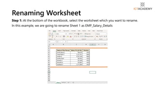
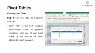
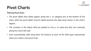
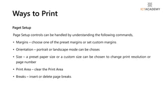
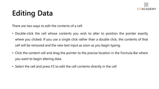
• From the Ribbon, choose Home  Cells  Format  Rename Sheet.
• Double-click the sheet tab.
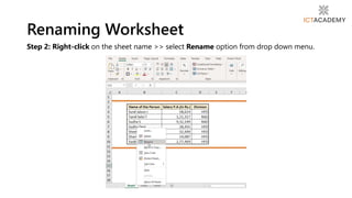
• Right-click the sheet tab and choose Rename Sheet.
• Sheet names may consist up to 31 characters, including spaces.
• However, the following characters are not permitted in sheet names:
• : (colon), / (slash), (backslash), [ ] (square brackets), ? (question mark), * (asterisk)
Changing name of a Worksheet

Step 1: Tap the Worksheet Tab. In the Home Tab in the Cell Group
Step 2: On the left, select Format, a drop-down menu will pop up.
Step 3: Select Tab Colour, now choose a Colour, or right-click the Worksheet Tab and
choose Tab Colour.
Step 4: When you look at the Worksheet Tab, its Colour does not look bright, but the Color
will show if you add another Worksheet Tab.
How to Change color of a Tab

To hide a worksheet
• Choose Home  Cells  Format  Hide & Unhide  Hide Sheet, or right-click its sheet
tab and choose Hide.
To Unhide a worksheet
• Choose Home  Cells  Format  Hide & Unhide  Unhide Sheet, or right-click its
sheet tab and choose Unhide.
Excel opens the Unhide dialog box, which lists all hidden sheets. Choose the sheet that you
want to redisplay, and click OK.
Hiding and Unhiding Worksheet

To insert a row or rows
• Select an entire row or multiple rows by clicking the row numbers in the worksheet
border. Right-click and choose Insert from the shortcut menu.
• Move the active cell to the row that you want to insert and then, Choose Home  Cells 
Insert  Insert Sheet Rows.
• When several cells in a column are chosen, Excel inserts new rows equal to the number of
cells selected and shifts the rows below the insertion down.
Inserting Rows

To insert a column or columns
• Select an entire column or multiple columns by clicking the column letters in the
worksheet border. Right-click and choose Insert from the shortcut menu.
• Move the active cell to the column that you want to insert and then, Choose Home 
Cells  Insert  Insert Sheet Columns.
• When many cells in a row are chosen, Excel inserts extra columns equal to the number of
cells selected in the row.
• You can also insert cells rather than rows and columns.
• Choose Home  Cells  Insert  Insert Cells.
Inserting Columns

To delete a row or rows
• Select an entire row or multiple rows by clicking the row numbers in the worksheet
border. Right-click and choose Delete from the shortcut menu.
• Move the active cell to the row that you want to delete and then, Choose Home  Cells
 Delete  Delete Sheet Rows.
• When numerous cells in a column are selected, Excel deletes all rows in the selection.
Deleting Columns works in similar way.
Deleting Rows and Columns

Use any one of the following
• With the mouse, drag the right-column border until the column reaches the required width.
• Choose Home  Cells  Format  Column Width and enter a value in the Column Width
dialog box
• Choose Home  Cells  Format  AutoFit Column Width to adjust with width of the selected
column so that the widest entry in the column fits. Rather of picking a full column, you may
just choose cells inside it, and the column is resized to match the width of the broadest entry
in your selection.
• Double-click the right border of a column header to automatically change the column width to
the width of the column's largest item.
Changing Column Width

Use any one of the following
• Drag the lowest row border to the desired height with the mouse.
• Choose Home  Cells  Format  Row Height and enter a value in the Row Height
dialog box
• Double-click the bottom border of a row to set the row height automatically to th tallest
entry in the row
• Also, Choose Home  Cells  Format  AutoFit Row Height.
Changing Row Heights

Copy and Paste
When you copy a cell, the selected cell data remains in its original location and is added in a
temporary storage area called the Clipboard.
Step 1: Select the cell or cell range you want to copy.
Step 2: Click the Copy button on the Home tab.
Cut, Copy, & Paste in Excel

Step 3: Click the cell where you want to paste your data.
Step 4: Click the Paste button.

Cut and Paste
When you cut a cell, its content is removed from the original location and placed in the
Clipboard.
Step 1: Select the cell or cell range you want to cut.
Step 2: Click the Cut button on the Home tab.
Step 3: Click the cell where you want to paste your data.
Step 4: Click the Paste button.

• Excel 2019 has a new tool called Format as Table that enables you to format a full range of
data in a single action. This can be done by clicking new style thumbnail found in the
Table Styles gallery
• When formatting tables, you can check the following items in the Table Style Options
group.
• Header Row, Total Row, Banded Rows, First Column, Last Column, Banded Columns
• Quick Analysis Tool can also be used to format tables.
• Simply pick the table cells, including the first row and column headers, and the tool will show in
the lower right corner. Then select the Tables tab to see your formatting options.
Formatting Tables

• Unwanted or uncommon values (values outside specific boundaries) can be automatically
formatted using the Conditional Formatting option.
• The Conditional Formatting button is located in the Styles thumbnail on the Home tab,
and it has the following options:
• Highlight Cells Rules - includes options for establishing formatting rules for cells with specific
values, dates, or text.
• Top/Bottom Rules - a menu with options for top and bottom numbers, averages, percentages,
etc.
• Data bars - is a set of coloured data bars that show the values of a cell selection.
Conditional Formatting

• Options (continued)
• Color Scales - By clicking the colour scale thumbnail, a palette with several coloured scales may
be used to show the values of a cell selection.
• Icon Sets - A palette of numerous icons that may be attached to a cell selection to signify
various circumstances that apply to certain threshold levels.
• New Rule - specify a custom conditional formatting rule that will be applied to the selected cell.
• Clear Rules - a continuation menu from which you may delete conditional formatting rules for
the selected cell.
• Manage Rules - leads you to the Conditional Formatting Rules Manager, where you may alter
specific rules and rearrange their priority.
Conditional Formatting

Printing from Backstage View
• Press Ctrl+P. Through this we can,
• Change the number of spreadsheet copies to be printed
• Click the name of the printer to use when printing the spreadsheet
• Choose the part of the spreadsheet to be printed – between Print Active Sheets, Print Entire
Workbook, or Print Selection
• Print both sides of the paper through the Print on Both Sides, Flip Pages on Long Edge, or Print
on Both Sides, Flip Pages on Short Edge options
• Change paper orientation from portrait to landscape or vice versa
• Change paper size, margins
Ways to Print

Quick Printing
• If you are familiar with Excel's basic print settings, you can print your spreadsheets quickly.
• Simply click the Customize Quick Access button and select the Quick Print item from the
menu to add the Quick Print button to the Quick Access Toolbar.
• After you've added the Quick Print button, you may use it to print a copy of the current
worksheet's whole contents.
• Excel passes the print job to the print queue and then sends it to the printer for
processing.
• To stop the printing, click Cancel in the Print dialog box
Ways to Print

Paget Setup
Page Setup controls can be handled by understanding the following commands,
• Margins – choose one of the preset margins or set custom margins
• Orientation – portrait or landscape mode can be choses
• Size – a preset paper size or a custom size can be chosen to change print resolution or
page number
• Print Area – clear the Print Area
• Breaks – insert or delete page breaks
Ways to Print

Paget Setup
Page Setup controls can be handled by understanding the following commands,
• Background – You may provide a graphic picture as the background image for all
worksheets in your workbook.
• Print Titles – You may define rows of the worksheet to repeat with the top columns
serving as print headlines for the report using the Sheet tab of the Page Setup.
Ways to Print

Using Print options
Print section of Page Setup box has useful options, these include:
• Gridlines
• Cell errors
• Comments
• Black and White
• Draft Quality
• Row and Column Headings
None of these settings are pre-selected, which means you may tamper with them if you wish to
improve the print quality of your worksheet.
Ways to Print

Page Break
Excel has a Page Break Preview tool that enables you to quickly identify and correct page
break issues. You can resolve similar issues by following the instructions below:
• Click the Page Break Preview button on the Status bar or Alt+WI
• Position the mouse pointer on the page break indicator
• After adjusting the page breaks, click the Normal button
Additionally, you may manually insert page breaks at the place of the cell cursor by
selecting Insert Page Break on the Page Layout tab (Alt+PBI) and removing them by
selecting Remove Page Break or (Alt+PBR).
Ways to Print

Entering Data
• To enter data into a cell, you must first activate it by
clicking on it.
• Then you may enter your data using one of two
methods:
• Begin typing and the text will display automatically inside
the cell.
• Access the Formula Bar by clicking it. As you type, the
data will populate the Formula Bar and the current cell.

Editing Data
There are two ways to edit the contents of a cell:
• Double-click the cell whose contents you wish to alter to position the pointer exactly
where you clicked. If you use a single click rather than a double click, the contents of that
cell will be removed and the new text input as soon as you begin typing.
• Click the content cell and drag the pointer to the precise location in the Formula Bar where
you want to begin altering data.
• Select the cell and press F2 to edit the cell contents directly in the cell

Enter a text or number in a Cell
• On the worksheet, click a cell
• type the numbers or text that you want to enter, and then press Enter or
Tab.
• To enter data on a new line within a cell, enter a line break by pressing
Alt+Enter.

Enter a number having fixed decimal
• On the File tab, click Options
• Click Advanced, and then under Editing options, select the Automatically insert a
decimal point check box
• In the Places box, enter a positive number four digits to the right of the decimal point or a
negative number for digits to the left of the decimal point.
• For example, if you enter 3 in the Places box and then type 3679 in a cell, the value will
appear as 3.679. If you enter a -3 in the Places box and then type 679, the value will be
679000.

Enter a number having fixed decimal
• On the worksheet, click a cell, and then enter the number that you want.
• Data that you typed in cells before selecting the Fixed decimal option is not affected.
• To temporarily override the Fixed decimal option, type a decimal point when you enter
the number.

Automatically moving the selection after
entering data
• By default, when you press the Enter key after
entering data into a cell, Excel automatically
picks the next cell below.
• To modify this setting, open File Options and
navigate to the Advanced tab (see image).
• The check box that controls this behavior is
labeled After clicking Enter, move selection.
• If this option is enabled, you can choose the
direction in which the selection advances
(down, left, up, or right).
Data-Entry Techniques

Selecting a range of input cells before entering data
• When a range of cells is chosen, hitting Enter automatically chooses the next cell in the range,
even if the After pressing Enter, move selection option is deactivated.
• If the selection spans many rows, Excel descends the column; when it reaches the end of the
column's selection, it advances to the first chosen cell in the next column.
• Simply hit Enter without inputting anything to skip a cell.
• To return to backward, press Shift+Enter.
• If you'd rather enter data by rows than columns, hit Tab instead of Enter.
• Excel will continue to cycle through the specified range until a cell outside the range is selected.
• The selected range can be changed using any of the navigation keys, such as the arrow keys or
the Home key. To travel inside the specified range, you must use Enter and Tab.

Using Ctrl+Enter to place information into multiple cells simultaneously
• If you need to enter the same data many times in different cells, Excel provides a convenient
shortcut.
• Select all of the cells that will hold the data; insert the value, text, or formula in each cell; and
then hit Ctrl+Enter.
• Each cell in the selection receives the same data.the Home key.
• To travel inside the specified range, you must use Enter and Tab.

Changing Modes
• You may switch between Enter and Edit modes by pressing F2.
• In Edit mode, you may use your arrow keys to navigate through the phrase and correct the
misspelt word.
• Additionally, you may use the Ctrl+arrow keys to move a word at a time rather than a
character at a time.
• By hitting F2 again, you can continue entering text in Edit mode or return to Enter mode,
from which the navigation keys can be used to travel to a new cell.

Entering decimal points automatically
• Select the Advanced tab in the Excel Options dialogue box.
• Select the Automatically Insert a Decimal Point check box and ensure that the Places box is
set to the amount of decimal places required for the data you're entering.
• When this option is enabled, Excel automatically calculates the decimal points for you.
• For instance, if two decimal places are specified, typing 12345 into a cell is read as 123.45.
• Simply clear the Automatically Insert a Decimal Point check box in the Excel Options dialog
box to restore normalcy.

Use AutoFill to enter a series of values
• Excel's AutoFill tool simplifies the process of adding a sequence
of numbers or text items into a range of cells.
• It makes use of the fill handle (the small box at the lower right of
the active cell).
• You can slide the fill handle to duplicate the cell or to finish a
series automatically.

Forcing text to appear on a new line within a cell
• If a cell has a large amount of text, you may force Excel to show it in many lines within the
cell by pressing Alt+Enter to begin a new line.
• When you insert a line break, Excel switches the cell's format to Wrap Text automatically.
• However, unlike automated text wrapping, your manual line break requires Excel to break
the text at a specified point inside the text, giving you more exact control over how the
text appears than if you rely on automatic text wrapping.

Using AutoCorrect
• You can use the AutoCorrect feature to create
shortcuts for commonly used words or phrases.
• Choose File -> Options and click Proofing tab. Then
click the AutoCorrect options button to display the
AutoCorrect dialog box
• In the dialog box, click the AutoCorrect tab, check
the Replace Text as You Type option, and then enter
your custom entries.
• You can set up as many custom entries as you like.

• An Excel spreadsheet is simply a collection of cells that you can use to enter data. Each
cell is given a name based on its position in the spreadsheet. The top-leftmost cell is
called cell A1. It’s the cell located in column A, row 1.
• For instance, you can click cell C1 and begin typing =A1+B1, as shown. Note how you
can see your formula in both the cell you’re typing in and the Formula Bar above the
column headings.
Create and Revise Formulas

• Constants
You can use hard-coded numbers directly in a formula. For example, you can enter = 5+10
directly into a cell to get the answer 15.
• Operators:
These include symbols that perform addition (+), symbols that perform multiplication (*),
symbols that compare values (>), and symbols that join values together (&). For example,
entering =15>10 into a cell returns TRUE as the result because 15 is indeed greater than 10.
Types of Values in Excel formulas

• Text strings
Any text string can be used as an argument in a formula as long as it’s wrapped in quotation
marks. For example, entering = "Microsoft“ & "Excel" in any cell results in the joined text
Microsoft Excel.
• Cell references
These include any value that points back to a single cell or range of cells. As you’ve already
seen, entering =A1+B1 in a cell tells Excel to use the values in those two cells in the formula.
Types of Values in Excel formulas

Operators used in Formulas
Operator Name
+ Addition
- Subtraction
* Multiplication
/ Division
^ Exponentiation
& Concatenation
= Logical comparison/equal to
> Logical comparison/greater than
< Logical comparison/lesser than
>= Logical comparison/greater than or equal to
<= Logical comparison/lesser than or equal to
<> Logical comparison/not equal to

Operators precedence in Formulas
Operator Name Precedence
^ Exponentiation 1
% Percent 1
* Multiplication 2
/ Division 2
+ Addition 3
- Subtraction 3
& Concatenation 4
= Equal to 5
< Less than 5
> Greater than 5

• Numerous formulae you construct make use of worksheet functions.
• These functions enable you to significantly increase the power of your formulas and
perform calculations that would be difficult (or even impossible) to perform using only
the operators previously discussed.
• To calculate average of the values in 10 cells (A1:A10) without function =
(A1+A2+A3+A4+A5+A6+A7+A8+A9+A10)/10
• This formula can be replaced with a simple function – AVERAGE “=AVERAGE(A1:A10)
Functions

A function may use one of the following,
• No arguments
• One argument
• A fixed number of arguments
• An indeterminate number of arguments
• Optional arguments
Function arguments

• No Arguments
• Example: NOW() – returns the current date and time.
• Even if a function does not take an argument, a set of empty parentheses must be provided.
• If a function takes more than one parameter, use a comma to denote each argument.
• A cell reference, literal values, literal text strings, expressions, and even other functions can
be used as an argument.
• Cell reference = MAX(A1,B1); Literal value = SQRT(144); Literal text string = UPPER(A2);
Expression = SUM(132+5); other functions = SQRT(SUM(A1:A12)
Function arguments

• Utilize Formula AutoComplete (the drop-down list that Excel displays while you type a
formula).
• To utilize this, at the very least the first character of the function's name must be known.
• Another way to insert a function is to use tools in the Function Library group on the
Formulas tab on the Ribbon
• This method is especially useful if you can’t remember which function you need.
Inserting Functions into Formulas

• Another way to insert a function is to use the
Insert Function dialog box. To access there are
several ways as given below,
• Choose Formulas  Function Library  Insert
Function
• Use the Insert function command, appearing at
the bottom of each drop-down list in the Formulas
 Function Library group
• Click the Insert Function icon (Formula bar fx)
• Press Shift+F3
Inserting Functions into Formulas

A cell reference in spreadsheet programs such as Excel and Google Sheets identifies the location
of a cell in the worksheet.
These references use Autofill to adjust and change information as needed in your spreadsheet.
Types of Cell References
• Relative cell references contain no dollar signs (i.e., A1).
• Mixed cell references have dollar signs attached to either the letter or the number in a
reference but not both (i.e., $A1 or A$1).
• Absolute cell references have dollar signs attached to each letter or number in a
reference (i.e., $A$1).
Cell References

• Cell references in formulas make it easier to copy formulas from one location to another
in a worksheet or workbook.
• Relative cell references change when copied to reflect the new location of the formula.
The name relative comes from the fact that they change relative to their location when
copied.
• Copying formulas is the other major use of an absolute reference such as =$A$2+$A$4.
The values in those references don't change when you copy them.
Cell References

• At other times, you may want part of a cell reference to change, such as the column letter,
while having the row number stay static or vice versa when you copy the formula. In this
case, you'll use a mixed cell reference such as =$A2+A$4. Whichever part of the reference
has a dollar sign attached to it stays static, while the other part changes when copied.
• So for $A2, when it is copied, the column letter is always A, but the row numbers change
to $A3, $A4, $A5, and so on.
• The decision to use the different cell references when creating the formula is based on the
location of the data that the copied formulas will use.
Cell References

To change existing cell references, Excel must be in edit mode, which you enter by double-
clicking on a cell with the mouse pointer or by pressing the F2 key on the keyboard.
To convert relative cell references to absolute or mixed cell references:
• Press F4 once to create a cell reference fully absolute, such as $A$6.
• Press F4 a second time to create a mixed reference where the row number is absolute,
such as A$6.
• Press F4 a third time to create a mixed reference where the column letter is absolute,
such as $A6.
• Press F4 a fourth time to make the cell reference relative again, such as A6.
Toggling between Cell References

Excel Error values
Error value Description
#DIV/0! The formula is attempting division by zero. Due to the fact that
Excel assigns a value of 0 to empty cells, this error also happens
when the formula attempts to divide by a blank or null cell.
#NAME? Excel does not recognize the name of the formula. This can occur if
you erase a name that is referenced in the formula, if you misspell
a name and then press Enter, or if you use text with mismatched
quotations.
#N/A The formula is referring to (directly or indirectly) a cell that utilizes
the NA function to indicate that no data is available.
#NULL! The formula uses an intersection of two ranges that don’t intersect.

Excel Error values
Error value Description
#NUM! There is an issue with a value; for instance, you supplied a negative
value as an input when a positive value is needed.
#REF! The formula refers to an invalid cell. This can occur if the
worksheet's cell has been erased.
#VAULE! The formula has an incorrect argument or operand. (An operand is
a value or a cell reference that is used by a formula to calculate the
outcome.)

Excel utilizes logical functions to identify mistakes. These functions are accessible via the
Logical command button on the Formulas tab of the Ribbon (Alt+ML). Syntax are,
• IF(logical_exp,value_if_true,value_if_false)
• evaluates whether the logical_exp expression is TRUE or FALSE. If TRUE, the IF function uses the
value_if_true argument and returns it to the cell. If FALSE, the IF function uses the value_if_false
argument and returns it to the cell.
• IFERROR(value,value_if_error)
• returns the value argument when the cell referred to in another logical argument in which the
IFERROR function is used doesn’t contain an error value and the value_if_error argument when it
does.
Logical Functions

• IFNA(value,value_if_na)
• returns the value argument when the cell referred to in another logical argument in which the
IFNA function is used doesn’t contain #NA and the value_if_error argument when it does.
• IFS(logical_test1,value_if_true1)
• evaluates whether or not one or more logical_test arguments are TRUE.
• AND(logical_exp1,logical_exp2,…)
• evaluates whether the logical_exp arguments are TRUE or FALSE. If all expressions are TRUE, the
AND function returns TRUE to the cell. If any of them are FALSE, the AND function returns
FALSE.
Logical Functions

• OR(logical_exp1,logical_exp2,…)
• evaluates whether the logical_exp arguments are TRUE or FALSE. If any expressions are TRUE,
the OR function returns TRUE. If all are FALSE, the OR function returns FALSE.
• XOR(logical_exp1,logical_exp2,…)
• evaluates whether the logical_exp arguments (usually in an array) are predominantly TRUE or
FALSE. When the number of TRUE inputs is odd, the XOR function returns TRUE. When the
number of TRUE inputs is even, the XOR function returns FALSE.
• TRUE( ) – returns TRUE in its cell without condition
• FALSE( ) – returns FALSE in its cell without condition
Logical Functions

• The Excel calendar began on 1 January 1900. That concluded as day one.
• Each succeeding day has been assigned a unique number. The number for the first day of
May 2018 is 43221.
• Times are treated as fractions of a day. 0.5 is noon, 0.25 is 6am and 0.75 is 6pm. When
dealing with times and durations such as hours and minutes, you are working with
fractions (decimals)
• Only when you enter a formatted date or time as a text entry into a worksheet should you
be concerned with converting them to time and date serial numbers that Excel may use to
do computations.
Date and Time

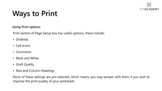
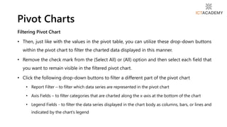
• Excel includes a variety of built-in date functions that you may use into your spreadsheet.
• Additionally, you may discover additional features when you install an add-in.
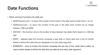
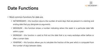
• Most common functions for date are,
• TODAY – this function has no arguments and is always entered as “=TODAY()”.
• DATE and DATEVALUE – has the following syntax: (DATE(year,month,day). the DATE function returns
a date serial number for the date specified by year, month, and day.
• DAY(serial_num) – to return the day of the month in the date
• WEEKDAY(serial_num,[return_type]) – to return the day of the week (as a number from 1 to 7 or 0
to 6). The optional return_type is a number between 1 and 3; 1 designates the first type (1-Sunday,
7-Saturday), 2 – second type (1-Monday, 7-Sunday) and 3 – third type (0-Monday, 6-Sunday)
Date Functions

• MONTH(serial_num) – to return the number of the month in the date serial number (from 1 to 12).
• YEAR(serial_num) – to return the number of the year in the date serial number (as an integer
between 1900 and 9999).
• DAYS360 – this function returns the number of days between two dates that’s based on a 360-day
year
• EDATE – (elapsed date) this function computes a past date or future date that is lots of months
ahead or behind the date that you designate as its start_date argument.
• EOMONTH – (end of month) this function computes the last day of the month that is either so
many months ahead or behind the date that you state as your start_date argument.
Date Functions

• NETWORKDAYS – this function returns the number of work days that are present in a starting and
ending date that you designate as arguments.
• WEEKNUM – this function shows a number indicating where the week in a particular date falls
within a year.
• WORKDAY – this function is used to find out the date that is so many workdays either before or
after a certain date.
• YEARFRAC – this function allows you to calculate the fraction of the year which is computed from
the number of days between dates.
Date Functions

• You can use the Time functions to convert text entries that represent times of day into time
serial numbers, which can then be used in calculations.
• Functions for merging sections of a time into a single serial number and extracting the
hours, minutes, and seconds from a single time serial number are also included in the Time
functions. Some are,
• NOW – this function displays the current date and time on your device.
• TIME AND TIMEVALUE – this function allows you to create a decimal number that represents a time
serial number, ranging from 0 to 0.99999999, and representing time 0:00:00 to 23:59:59.
• HOUR, MINUTE, and SECOND – these functions enable you to extract segments of a time value
from a spreadsheet.
Time Functions

What Is a Chart?
• A chart is a visual representation of numeric values.
• Charts (also known as graphs) have been an integral part of spreadsheets since the early
days. Charts generated by early spreadsheet products were extremely crude by today’s
standards.
• Displaying data in a well-conceived chart can make your numbers more understandable.
Getting Started with Excel Charts

Eg: The Figure shows a worksheet that contains a simple column chart that depicts a
company’s sales volume by month.
Getting Started with Excel Charts

• Typically, the data for a chart is contained within a single worksheet, however this is not a
necessity.
• A chart can access data from any number of worksheets, and the worksheets themselves
can be located in various workbooks.
• Whether to use data from a single sheet or numerous sheets is entirely dependent on your
data model, the nature of your data sources, and the level of interactivity desired for your
dashboard.
• This item is composed of one or more data series that are visually represented. The look of
the data series is determined on the chart type used.
• For instance, if you build a line chart with two data series, the chart will include two lines,
each representing a different data series. Each series' data is recorded in its own row or
column.
How Excel handles charts

• Line chart displaying two data series

• A key point to keep in mind is that charts are dynamic.
• If the data changes, the chart is immediately updated to reflect the change, ensuring that
your dashboard always displays the most up-to-date information.
• Charts can reside in either of two locations in a workbook:
• On a worksheet (an embedded chart)
• On a separate chart sheet

• An embedded chart floats on top of a worksheet, on the drawing layer of the worksheet.
• As with other drawing objects (such as a text box or a shape), you may move, resize, modify
the dimensions of, and edit the borders of an embedded chart, as well as apply effects such
as a shadow.
• By embedding charts, you may examine the chart with the data it utilises.
• Alternatively, you may group together numerous embedded charts to publish on a single
page.
• To make any modifications to the embedded chart object's actual chart, you must click it to
activate it.
Embedded Chart

• You can move an embedded chart to its own chart sheet so that you can view it by clicking
a sheet tab.
Embedded Chart

• This particular chart is a
combination chart that
displays both columns and
a line.
• The chart has two data
series: Income (vertical
columns) and Profit Margin
(line with square markers)
Parts of a Chart

• Funnel charts are great for displaying relative numbers at different stages of a process.
• Value axes are what they're called, and each one has a distinct scale.
• The left axis represents the column series (Income), whereas the right axis represents the
line series (Profit Margin).
• Scale values range from 0 to 250,000, with major unit increments of 50,000 on the left
axis. The right-hand value axis employs a different scale, ranging from 0% to 14% in 2%
increments.
• The chart's legend is located at the bottom. The example chart indicates the Profit
Margin series but not the Income series.
Parts of a Chart

Step 1: Select the data you want to use in the chart
(sample below)
Step 2: Click the Insert tab and then click a Chart icon
(appropriate to you) in the Charts group
Steps for creating a Chart

Step 3: Click the Chart subtype, and Excel then creates the chart of the specified type
(sample given)
Steps for creating a Chart

• When Excel constructs a chart, it determines whether the data should be organized in
columns or rows using an algorithm.
• While Excel frequently makes the correct assumption, if it builds the chart with the
incorrect orientation, you can immediately adjust it by selecting the chart and choosing
Chart Tools Design  Data  Switch Row/Column.
• This is a toggle command; if changing the data orientation does not enhance the chart,
simply pick it again (or click the Undo button found on the Quick Access toolbar).
Switching row and column

• You can choose Chart Tools Design  Type  Change Chart Type to display the
Change Chart Type dialog box and experiment with other chart types
Changing Chart Type

• To give a Chart Title, choose Chart Tools  Design Add Chart Elements  Chart Title
Adding/Deleting chart elements

• If your chart is embedded, you may drag and resize it freely with your mouse.
• When a chart is selected, you may alter the chart's height and width using the Chart
Tools Format  Size settings.
• To resize an embedded chart, just click anywhere on its border other than one of the
eight resizing handles. The chart will then be dragged to its new place.
• Additionally, you may relocate an embedded chart using typical cut and paste
procedures.
Resizing Chart

• To edit the data of chart, click Select Data on the Design tab of the Chart tools
• Select Data Source dialog box will be opened which enables the below modifications
• Adjust/modify the data range being graphed
• Change the column and row headers
• Edit the legend's labels to include the data series' names.
• Add a new series of data to the chart.
• Remove a label from the legend
• Rearrange the data series
• Demonstrate how to handle empty cells in a data range.
• Explicitly display data in Hidden Rows and Columns
Editing Chart’s source data

• To convert an embedded chart to a chart on a chart sheet, select the chart and choose
Chart Tools Design  Location  Move Chart to display the Move Chart dialog box
Embedded chart to Chart sheet

Copying a Chart
• Select the chart and choose Home  Clipboard  Copy (or press Ctrl+C). Then activate
a cell near the desired location and choose Home  Clipboard  Paste (or press
Ctrl+V).
Deleting a Chart
• To delete an embedded chart, Click the chart and then press Delete
• When the Ctrl key is pressed, you can select multiple charts and delete all with single
press of the Delete key

Adding Chart Elements
• To add new elements to a chart (such as a title, legend, data labels, or gridlines),
activate the chart and use the controls in the Chart Elements + icon, which appears to
the right of the chart.
• You can also use the Add Chart Element control on the Chart Tools Design tab, in the
Chart Layouts group

Example: Same data
plotted using Six Chart
Types

• Essentially, a bar chart is a column chart that has been spun 90 degrees clockwise.
• One notable advantage of a bar chart is that the category labels may be more legible.
Bar Chart

• They are used to visualize continuous data and are particularly good for finding
patterns.
Line Chart

• Another common chart type is an XY chart (also known as scatter grams or scatter plots).
• An XY chart differs from most other chart types in that both axes display values. (An XY
chart has no category axis.)
XY (scatter) Chart

• Think of an area chart as a line chart in which the area below the line has been colored in.
Area Charts

• A radar chart is a customized chart in which each category has its
own axis, which extends outward from the chart's centre.
• Each data point's value is shown on the corresponding axis.
Radar Charts

• It displays two or more data series on a surface.
• If you have data in the form of x, y, and z coordinates, it cannot be correctly displayed on a
surface chart unless the x and y values are evenly spaced.
Surface Charts

• Think of a bubble chart as an XY chart that can display an additional data series, which is
represented by the size of the bubbles.
• As with an XY chart, both axes are value axes. (There is no category axis.)
Bubble Charts

• Stock charts are extremely useful for visualizing market data. Three to five data series are
required for these charts, depending on the subtype.
Stock Charts

• A histogram displays the count of data items in each of several discrete bins.
• With a bit of effort, you can create a histogram by using a standard column chart or by
using the Analysis ToolPak.
Histogram Charts

• The Pareto chart type is actually a Histogram subtype. You can find the Pareto chart type
under Charts  Insert Statistic Chart.
• It is a combination chart in which columns are displayed in descending order, and the
columns use the left axis.
Pareto Charts

• Typically used to illustrate the cumulative effect of a succession of integers, both positive
and negative.
Waterfall Charts

• A two-column table contains the data.
• Vertical lines extending from the box reflect
the numerical range of the data in the chart
(minimum and maximum values).
• The median value is indicated by the
horizontal line inside the box, while the
average is indicated by the X.
• This chart format helps the user to quickly
compare groupings of data.
Box & Whisker Charts

• A sunburst chart is like a pie chart with multiple concentric layers.
• This chart type is most useful for data that’s organized hierarchically.
Sunburst Charts

• A treemap chart, like a sunburst chart, is well-suited for hierarchical data. However, the data
is displayed as rectangles.
Treemap Charts

• Funnel charts are an excellent way to illustrate the relative values at each stage of a process.
Funnel Charts

Controlling Graphics
• When interacting with objects, the mouse cursor transforms into a double-headed arrow
that you may drag to change the overall size and shape of the item.
• Additionally, you may limit a graphic while resizing it by clicking the scaling handle and
then dragging while pressing and holding the Shift key.
• 2-D rotation
• When the pointer is on a 2-D rotation handle, it turns into a clockwise curving arrow.
• When you're ready to drag the 2-D rotation handle, the pointer changes to four curving arrows in
a clockwise circle.
• From there, you may rotate the graphic with the rotation handle.
Graphic Objects

• 3-D rotation
• When the pointer is in a 3-D rotation handle, it turns into a clockwise circular arrow.
• The item may then be rotated in 3D space to be seen from any angle: above, below, in front,
behind, or on either side.
• Hold down the Ctrl key while dragging the graphic to duplicate it.On a touchscreen device,
use your finger or stylus to rotate, resize, or shape a graphic object.
Graphic Objects

Moving graphic objects to different layers
• Objects on your spreadsheet may also be layered. This implies that if you drag a graphic
over a cell with data, the graphic hides the data beneath it.
• Using the Selection task pane in Excel, you may transfer graphic objects across levels.
• Simply click the object's name and drag it up or down in the task window.
• To move the item, utilize the Bring Forward or Send Backward buttons.
Graphic Objects

Different Types of Graphics
• Graphics may be used on spreadsheets in Excel and further customized using the
Illustration button on the Insert tab.
• These include,
• Pictures
• Online pictures
• Shapes
• Icons
• 3-D Models
• SmartArt
• Screenshot
Graphic Objects

Inserting online images
• To insert 2-D online pictures, open the Online Pictures dialogue box or press Alt+NF, then
select one of the categories offered or use the Select Bing text box to input the image's
keyword.
• This dialogue box displays a scrollable list of photographs that match your keyword.
• Then click on any thumbnail to view its description and size.
• Download the images and store in local drive or any file storage service (Google drive or
OneDrive)
• Once you click the browse button, Excel will show you a list of folders from which you may
choose the picture you wish to use on your worksheet.
Graphic Objects

Inserting local images
• You may like to incorporate a picture into your worksheet, such as a digital photo or a
scanned image that is locally saved on your computer.
• This may be accomplished by selecting Pictures from the Illustration's drop-down menu, or
by pressing Alt+NP.
Graphic Objects

Drawing Shapes
• To begin sketching shapes, navigate to the Shapes gallery and then select from a large
number of premade shapes by dragging the mouse pointer to a thumbnail of the desired
shape.
• Following that, click the thumbnail of the preset form and drag it into the worksheet until it
reaches the desired size.
Adding text boxes
• To create a text box, click the Text Box button (Alt+ NX) on the Insert tab.
• Then drag the pointer's mouse to the new text box's outline.
• When you release the mouse button, Excel creates the text box and inserts an insertion
point into which you may type the text to be displayed.
Drawing Graphic Objects

WordArt
1. Click the WordArt button or Alt+NW
2. Click the thumbnail in the WordArt style that you want to use
3. Type the text that you want on the worksheet in the text box
4. To format the text box’s background, use Live Preview in the Shape styles drop-down and
find your required style
5. After final adjustments to size, shape or orientation of the WordArt text, click a cell outside
of the text to deselect

SmartArt Graphics
• SmartArt graphics enable you to create elaborate diagrams and descriptive images directly
on your worksheet.
• To enter a SmartArt graphic, click the SmartArt button or Alt+M1, then select a category
from the left-hand navigation pane, followed by the thumbnail of the SmartArt graphic
you wish to use, and then click OK.

• When you link two sheets together, data is dynamically pulled from one into the other and
updated in the destination sheet whenever the contents of a cell in the source sheet
changes.
Step 1: Open a Microsoft Excel workbook.
Link Sheets

Step 2: Click an empty cell in your destination sheet. This will be your destination cell. When
you link it to another sheet, the data in this cell is synced and updated automatically whenever
the data in the source cell changes.
Link Sheets

Step 3: Type = in the cell. It will start a formula in your destination cell.
Link Sheets

Step 4: Click your source sheet from the sheet
tabs. Check the formula bar.
• The formula bar at the top of your workbook
displays the value of the destination cell.
• When you transition to your source sheet, it
should display the current worksheet's name,
followed by an equals sign and an exclamation
point.
Link Sheets

Step 5: Click a cell in your source sheet. This will
be your source cell.
• It might be an empty cell or one that contains
data.
• When you link sheets, the data in the
destination cell is updated automatically with
the data in the source cell.
Link Sheets

Step 6: Click ↵ Enter on your keyboard.
• This completes the calculation and returns you
to the destination sheet.
• Your destination cell is now connected to the
source cell and dynamically populates it with
data.
• When you make changes to the data in your
source cell, the data in your destination cell is
likewise updated.
Link Sheets

Step 7: Click your destination cell. This will highlight the cell
Link Sheets

• When dealing with a collection of identically formatted sheets, grouping them together
might save you some time.
• Once the spreadsheets are combined, you may enter identical data, make identical
modifications, create identical formulae, and apply same formatting to all of them.
• To group sheets in Excel, hold down the Ctrl key and click the sheet tabs of interest one
by one. After clicking the last tab, release Ctrl.
• To group adjacent (consecutive) worksheets, click the first sheet tab, hold down the
Shift key, and click the last sheet tab.
Group and Ungroup Worksheets

• There are two visual signs of grouped worksheets in Excel:
• The sheet tabs in a group have a white background; the sheet tabs outside the group
appear in grey.
Grouped Worksheets

To group all the worksheets in a workbook, this is what you need to do:
• Right-click any sheet tab.
• Choose Select All Sheets in the context menu.
Group all Worksheets

Worksheets can be ungrouped in this way:
Step 1: Right-click any sheet tab in the group.
Step 2: Choose Ungroup Sheets in the context menu.
Ungroup Worksheets

• Formatting in Excel is a technique that we may use to alter the presentation of data in a
spreadsheet.
• We may format the data in a variety of ways, for example, by using the styles and format
option on the Home page to change the font of the cells or the table.
• Excel formatting is an optional process that follows data preparation, which includes
data cleansing, structure, enrichment, and standardization.
Formatting

The following are some of the benefits of Excel data formatting:
• The data seems more aesthetically pleasing.
• Formatting data significantly reduces time and effort.
• We may analyze the data with the chart's assistance.
• We may use formatting to draw attention to certain data points in a firm, such as profit
or loss.
Benefits of Formatting

• In Excel, the format cells is used to modify the formatting of cell numbers without
modifying the actual number.
• With the help of the format cells, we can change the number, alignment, font style,
Border style, Fill options, and Protection.
Formatting Cells

• The Excel Number Tab is used to modify the decimal formatting of number cells,
providing the suitable format for numbers, dates, percentages, and fractions.
• The Number Tab enables us to format the numbers according to our specifications. We
may pick from a variety of options, including currency, dates, hours, and percentages.
Number Tab

• The alignment tab may be used to align the text in a cell and to combine the content in
two cells.
• If the text is hidden, we may use the wrap text function to properly show it and align it in
the desired direction.
• The Alignment tab of the Formal cells dialogue box enables us to determine how our
values are positioned horizontally and vertically.
Alignment Tab

• We may change the font size, font style, and font colour using the Font Tab. We may
alter the font's effects, underline the text, and examine the final result.
• While the main tab allows for quick font changes, the Formal Cells dialogue box is more
efficient for bulk adjustments.
• From there, we can simply change the typeface, font size, italicization, point size, bold
underlining, italicization, and colour of the entire selection of cells.
Font Tab

• We may construct colourful border lines for various designs by utilizing the Border Tab; if
we don't want to offer a border outline, we can leave it blank.
• In Excel, we may draw boundaries around a single cell or a collection of cells.
• We may specify the line thickness, colour, and style, as well as the location of the lines
(for example, only on the cell's top or on all horizontal sides).
Border Tab

• The Protection tab allows you to safeguard a cell, a range of cells, a sheet, or a formula.
• Unless we've already protected our worksheet, the Protection tab is not applicable.
• To do so, click Protection in the Tools menu, then pick Protect Sheet. Finally, tick the
Contents check box to specify how the worksheet will be protected.
Protection Tab

• Here are the steps to combine multiple worksheets with Excel Tables using Power Query:
Step 1: Go to the Data tab
Consolidate data from multiple sheets

Step 2: In the Get & Transform Data group, click on the ‘Get Data’ option

Step 3: Go the ‘From Other Sources’
option.
Step 4: Click the ‘Blank Query’ option.
This will open the Power Query editor

Step 6: Hit the Enter key.
This will display the names of all the tables in the worksheet (along with any named ranges
and/or connections that exist in the workbook).

Data lists have a structure that you may customize using the Data tab's extensive collection of
commands.
Designing a Data List
• When creating a data list, you simply put the names of the fields you wish to track in the
worksheet's top row.
• Following that, add the data record beneath each field and structure the two rows of data into a
table.
• When naming fields, bear in mind that each entry in the list is unique, so keep them brief.
• Similarly, you may use the Wrap Text command button to align the field name in the cell such that
the text wraps to a new line.
• Additionally, it is important to avoid using numbers or formulae that display values as field names.
Basics of Data Lists

Steps to set up data list,
1. Select the blank cell in which you want to begin the new data list and then type the field
names for the objects you wish to track.
2. Make the initial entries in the columns underneath the row that contains the field names.
3. Click Format as Table, then click a thumbnail of one of the styles in the drop-down list
4. Click OK to close
Adding records to data list
• After creating the field names and one record in the data list, you may start adding records in
the following rows.
• To achieve this, just hit Tab while the cursor is in the final cell of the first record.

Eliminating duplicates
• Use the Eliminate Duplicates tool to remove duplicate records from your database, especially
if you have a huge data list with several persons entering data.
• Follow these steps,
• Position the cursor in one of the cells in the data list.
• Click the Remove Duplicates button on the Data tab or press Alt+AM.
• Remove all check marks from all fields in the Columns list box except those whose duplicates are
the reason for the record's removal.
• By clicking OK, the Remove Duplicates dialogue box will close and the duplicate records will be
removed from the specified list.

Data Sorting
• After creating and populating a data list, you may sort the records.
• You may define whether the sort should be ascending or descending, as well as additional
choices using the Sort drop-down list.
• Excel organizes text and information in ascending order from smallest to biggest. If you
choose descending order, Excel organizes the text from Z-A and the data from largest to
smallest.
• You may also sort by date, but remember that ascending order puts records oldest to newest,
while descending order puts records newest to oldest.

• In Excel, click inside the cell atop the column you want to sort.
• In our example, we’re going to click cell D3 and sort this column by salary.
Sort Data

Step 1: From the “Data” tab on top of the ribbon, click “Filter.”
Sort Data

Step 2: Atop each column, you’ll now see an arrow.
Step 3: Click the arrow of the column you wish to sort to bring up a menu that enables us to
sort or filter the data.
Sort Data

Step 4: The most straightforward method of sorting data is from smallest to greatest or
greatest to smallest, providing you have numerical data.
Step 5: In this situation, we're sorting salaries, so we'll choose the top option to sort from
smallest to largest.
Sort Data

Filtering Data
• Excel lets you filter your data list to only reveal the information you need.
• You can achieve this by using AutoFilter, which conceals data you don't want to view and only
shows records you want to see.
• But often, especially when employing calculated criteria, the AutoFilter function isn't
adequate to accomplish extensive data filtering.
Filters

AutoFilter
• Excel's AutoFilter makes filtering simple.
• To do so, click the AutoFilter button on the column you wish to filter data on, and then select
the criteria from the drop-down box.
• If your worksheet data list doesn't include AutoFilter buttons next to the field names, you may
show them by clicking the Filter button on the Data Tab or Ctrl+Shift+L.
Filters

Basic Filtering
• Every entry in that column has its own checkbox in the AutoFilter drop-down menu.
• Clear the check boxes for the entries whose records you don't wish to see.
• For each record you wish to show, uncheck the check box in front of it, then select each box
holding the entry for it.
• Click OK to close the AutoFilter drop-down list
Filters

• When working with a large database, a filter is unavoidably necessary.
• As a commonly used tool, the filter reduces a complex perspective to a simple one.
• To apply filters, the dataset must have a header row including the column names.
Filters

Step 1: Select the data and click “filter” under the “sort and filter” drop-down.
Filters

Step 2: The filters are added to the selected data range.
The drop-down arrows, shown within the red boxes in the following image, are filters.
Filters

Step 3: Click the drop-down arrow of the column “city” to view the different names of the cities.
Filters

Step 4: To see the invoice values of “Delhi” only, select “Delhi” and uncheck all the remaining
boxes.
Filters

After filtering a range in a worksheet, we can save the filter view as a custom view, and then
restore the filter view easily in Excel.
Step 1: Filter the range in Excel whose filter view you will save later.
Step 2: Click the View  Custom Views.
Save Custom Filter Criteria

Step 3: In the opening Custom Views dialog box, click the Add button.
Step 4: In the Add View dialog box, type a name for this filter view in the Name box, and click
the OK button.
Save Custom Filter Criteria

When you sort data using the sort dialog box, you get an option to add multiple levels to it.
Here are the steps to do multi-level sorting using the dialog box:
Step 1: Select the entire data set that you want to sort.
Step 2: Click the Data tab.
Step 3: Click on the Sort Icon (the one shown below). This will open the Sort dialog box
Multi-level Data Sorting

Step 4: In the Sort Dialogue box, make the following selections
• Sort by (Column): Region (this is the first level of sorting)
• Sort On: Values
• Order: A to Z
Multi-level Data Sorting

• Validation of data is a feature that restricts what a user may enter into a cell.
• It merely displays a notice to the user informing them of what is and is not permitted.
• Data validation enables you to accomplish a variety of tasks, such as creating lists of items
that include values that are not permitted in a cell or range of cells.
Example:
• We have a form with following columns – Name, Gender, Address, Telephone and date of
birth.
Data Validation

• Lets assume, we want the telephone column to carry only whole numbers with precisely 10
digits.
• Select the Telephone column,
• Click on the ‘Data’ tab
• In the ‘Data Tool’ group, click on ‘Data Validation’ to open the Data Validation Window.
Data Validation

• On the Data Validation box, Select ‘Allow’ drop-down menu and select ‘Whole Number’.
• Click on the ‘Data’ tab
• In the ‘Data Tool’ group, click on ‘Data Validation’ to open the Data Validation Window. Under ‘Data’
select ‘equal to’ and keep the value as 10
• Click on ‘Input Message’ and type in the title and input message that should pop up when a cell within
the telephone column is selected
• Move to the error alert and key in the message that should pop up as an alert if an invalid data is
entered.
• In Gender column, we can create a list and make it ‘Male’ or ‘Female’ or ‘Other’. Select ‘List’ from the
‘Allow’ drop-down, next, type in the data separated by comma. Finally enter input information and alert
that should be displayed when a wrong item is selected
Data Validation

• In Gender column, we can create a list and make it ‘Male’ or ‘Female’ or ‘Other’. Select ‘List’ from
the ‘Allow’ drop-down, next, type in the data separated by comma. Finally enter input information
and alert that should be displayed when a wrong item is selected
Data Validation

• Pivot tables are especially handy if you have a large number of rows or columns that contain
information that you need to manage and compare quickly.
• The term "pivot" refers to the ability to rotate (or pivot) the data in a pivot table in order to
examine it from a new viewpoint.
• To be clear, when you create a pivot table, you are not adding to, removing from, or
otherwise altering your data.
• Rather than that, you're merely restructuring the data to get relevant information.
• Working with a PivotTable is similar to investigating a strange object. In this case, the object
happens to be your data.
Pivot Tables

Creating Pivot Tables
Step 1: Enter your data into a range of rows and columns
• Each pivot table in Excel begins with a standard Excel table that contains all of your data.
• Simply insert your data into a predefined set of rows and columns to create this table.
• Utilize the highest row or column to categorize your data according to what they represent.
Pivot Tables

Step 2: Sort your data by a specific attribute
• Once you've input all of the data you want into your Excel sheet, you'll want to organize it in
some way to make it easier to handle once it's converted to a pivot table.
• To sort your data, pick the "Data" tab in the top navigation bar and then the "Sort" symbol.
• In the resulting window, you can choose to sort your data by any column and in any order.
• To sort your Excel sheet by "Views to Date," for example, choose this column heading under
"Column" and then choose whether to organize your posts in ascending or descending order.
Pivot Tables

Step 2: Sort your data by a specific
attribute
• Select "OK" in the Sort window's
bottom-right corner to properly
reorganize each row of your Excel
sheet by the amount of views
obtained by each blog post.
Pivot Tables

Step 3: Highlight your cells to create your pivot table
• After entering data into your Excel worksheet and sorting it according to your
preferences, mark the cells you want to summarize in a pivot table.
• Select the "PivotTable" icon from the "Insert" menu on the top navigation bar.
• Additionally, you may right-click anywhere on your worksheet, choose "PivotTable," and
manually specify the range of cells to include in the PivotTable.
• This will open an option box where, in addition to specifying the cell range, you can
choose whether to start the pivot table in a new worksheet or maintain it in the current
one.
Pivot Tables

• When you start a new sheet, you may move to and from it using the navigation bar at the
bottom of your Excel file.
• Once you've made your selection, click "OK.“
• Alternatively, you may highlight your cells, click the "Recommended PivotTables" button
to the right of the PivotTable icon, and open a pivot table with pre-set recommendations
on how to organize each row and column.
Pivot Tables

Pivot Tables

Step 4: Drag and drop a field into the “Row Labels” area
• Excel will build a blank pivot table for you once you've finished Step 1.
• The next step is to drag and drop a field into the "Row Labels" section, labelled with the
names of the columns in your spreadsheet.
• This determines which unique identifier - blog post title, product name, and so on - will
be used to arrange your data in the pivot table.
• For instance, suppose you wish to categorize a large amount of blogging data by post
title. Simply click and drag the Title field into the "Row Labels" box to do this.
Pivot Tables

Step 4: Drag and drop a field
into the “Row Labels” area
Pivot Tables

Step 5: Drag and drop a field into the
“Values” area
• After deciding how your data will
be organized, the following step is
to add some values by dragging a
field into the "Values" box.
• Continuing with the example of
blogging data, suppose you wish to
summarize blog post views by title.
Simply drag the "Views" field into
the Values box to do this.
Pivot Tables

Step 6: Calibrating Calculations
• By default, the total of a certain value is computed, but you may simply alter this to an
average, maximum, or lowest number depending on what you're calculating.
• To open the menu, click on the little upside-down triangle next to your value and select
"Value Field Settings.“ (1)
Pivot Tables

To assist you in orienting yourself, refer to the
accompanying diagram.
Column Labels
• A column-oriented field in the PivotTable.
• Each row in the field corresponds to a column.
Customer is a column field that includes two
elements in the illustration (Existing and New).
• You can have column fields that are nested.
Pivot Tables - Terminology

Grand Totals
• A row or column in a PivotTable that provides totals for all cells in that row or column.
• You can indicate whether grand totals for rows, columns, both, or none should be
calculated.
• In the illustration, the PivotTable displays grand totals for both rows and columns.
Group
• A group of objects that are considered as a single item. You may manually or automatically
group objects (group dates into months, for example).
• The PivotTable depicted in the illustration lacks specified groupings.

Item
• A field element that appears in a PivotTable as a row or column header.
• Existing and New are items in the Customer field depicted in the illustration.
• Three branches are included in the Branch field: Central, North County, and Westside.
• AcctType contains four sub-categories: Certificate of Deposit, Checking, Individual
Retirement Account, and Savings.
Refresh
• After making changes to the source data, recalculates the PivotTable.

Row Labels
• In the PivotTable, a field with a row orientation.
• Each item in the field is represented by a single row.
• Row fields can be nested. Both Branch and AcctType are depicted in the illustration as row
fields.
Source Data
• The data that was utilized to generate the PivotTable. It can be contained within a
worksheet or a separate database.

Subtotals
• A row or column in a PivotTable that provides subtotals for detail cells in that row or column.
• Below the data in the picture, the PivotTable provides subtotals for each branch.
• Additionally, you may display or hide subtotals above the data. A subtotal is labelled with the
item's name and the term Total.
Table Filter
• A PivotTable field with a page orientation that is used to restrict the data that is summarized.
• You can display a single item, a collection of things, or all items in a page field simultaneously.
OpenedBy indicates a page field that displays All in the illustration (that is, not filtered).

Values Area
• The cells that comprise a PivotTable's summary data.
• Excel provides numerous methods for summarizing data (sum, average, count, and so on).

Creating Pivot Charts
• On the Analyze tab, inside the PivotTable Tools contextual tab, click the PivotChart
command button in the Tools group or Press Alt+JTC
• Excel displays the Insert Chart dialogue box, which allows you to specify the type and subtype of
pivot chart to generate.
• In the Insert Chart dialogue box, select the thumbnail of the subtype of chart you wish to
create and then click OK.
• Excel inserts a pivot chart into the worksheet holding the pivot table.
• This new pivot chart has drop-down buttons for each of the pivot chart's four distinct sorts of
fields (Report Filter, Legend Fields, Axis Fields, and Values).
Pivot Charts

Creating Pivot Charts
• These drop-down options allow you to sort and filter the data displayed in the chart.
• Additionally, Excel replaces the PivotTable Tools contextual tab on the Ribbon with PivotChart
Tools.
• This PivotChart Tools tab is then separated into three tabs: Analyze, Design, and Format, the last
of which is selected automatically.
Pivot Charts

Moving Pivot Charts to its own sheet
Although Excel produces new pivot charts automatically on the same worksheet as the pivot table, you
may find it simpler to customize and work with the chart if you transfer it to its own chart page in the
workbook.
• Click the Analyze tab under the PivotChart Tools contextual tab to bring its tools to the Ribbon and
then click the Move Chart command button or press Alt+JTV. (Move Chart dialog box appears)
• Click the New Sheet button
• Rename the sheet name in the text box with more descriptive name
• Click OK to close the Move Chart dialog box and open the new Chart sheet with pivot chart
Pivot Charts

Filtering Pivot Chart
• The pivot table's Row labels appear along the x- or category-axis at the bottom of the
chart, while the pivot table's Column labels become the data series shown in the chart's
legend.
• The numbers in the Values field are plotted on the y- or value-axis that runs vertically
along the chart's left side.
• Excel automatically adds drop-down list buttons to each of the field types represented
when you create a new pivot chart.
Pivot Charts

Filtering Pivot Chart
• Then, just like with the values in the pivot table, you can utilize these drop-down buttons
within the pivot chart to filter the charted data displayed in this manner.
• Remove the check mark from the (Select All) or (All) option and then select each field that
you want to remain visible in the filtered pivot chart.
• Click the following drop-down buttons to filter a different part of the pivot chart
• Report Filter – to filter which data series are represented in the pivot chart
• Axis Fields – to filter categories that are charted along the x-axis at the bottom of the chart
• Legend Fields - to filter the data series displayed in the chart body as columns, bars, or lines and
indicated by the chart's legend
Pivot Charts

Using Spreadsheets.pptx

Recommended

Recommended

More Related Content

What's hot

What's hot (20)

Similar to Using Spreadsheets.pptx

Similar to Using Spreadsheets.pptx (20)

Recently uploaded

Recently uploaded (20)

Using Spreadsheets.pptx