DBMS Notes ssit College -kavya R

1. UNIT-3-DBMS-22AM5.2
SSIT-TUMKUR
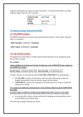
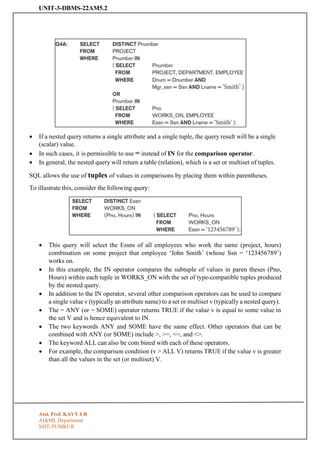
CREATE SCHEMA COMPANY AUTHORIZATION ‘Jsmith’;
Syntax:-CREATE TABLE EMPLOYEE
Subject: DATABASE MANAGEMENT SYSTEM
Subject Code: 22AM502
UNIT-3
Basic SQL: Data Definition and Data Types, Specifying constraints in SQL, Basic retrieval queries in
SQL, Insert, Delete and Update statements in SQL. More complex SQL Queries, Specifying Constraints
as Assertions and Actions as Triggers Views (Virtual Tables) in SQL, Schema change statements in SQL.
(Text 1: 6.1 to 6.4) (Text 1: 7.1 to 7.4)
6.1 SQL Data Definition and Data Types
6.1.1 Schema and Catalog Concepts in SQL
• For example, the following statement creates a schema called COMPANY owned by the
user with authorization identifier ‘Jsmith’. Note that each statement in SQL ends with a
semicolon.
• catalog—a named collection of schemas.
6.1.2 The CREATE TABLE Command in SQL
• The CREATE TABLE command is used to specify a new relation by giving it a name and
specifying its attributes and initial constraints.
Asst. Prof. KAVYA R
AI&ML Department

2. UNIT-3-DBMS-22AM5.2
SSIT-TUMKUR
6.1.3 Attribute Data Types and Domains in SQL
• The basic data types available for attributes include numeric, character string, bit
string, Boolean, date, and time.
1) Numeric data types include integer numbers of various sizes (INTEGER or INT, and
SMALLINT) and floating-point (real) numbers of various precision (FLOAT or REAL,
and DOUBLE PRECISION).
2) Character-string data types are either fixed length—CHAR(n) or CHARACTER(n),
where n is the number of characters—or varying length— VARCHAR(n) or CHAR
VARYING(n) or CHARACTER VARYING(n), where n is the maximum number of
characters.
Asst. Prof. KAVYA R
AI&ML Department

3. UNIT-3-DBMS-22AM5.2
SSIT-TUMKUR
CHECK (Dept_create_date <= Mgr_start_date);
3) Bit-string data types are either of fixed length n—BIT(n)—or varying length— BIT
VARYING(n), where n is the maximum number of bits.
4) A Boolean data type has the traditional values of TRUE or FALSE.
5) The DATE data type has ten positions, and its components are YEAR, MONTH, and
DAY in the form YYYY-MM-DD. The TIME data type has at least eight positions,
with the components HOUR, MINUTE, and SECOND in the form HH:MM:SS.
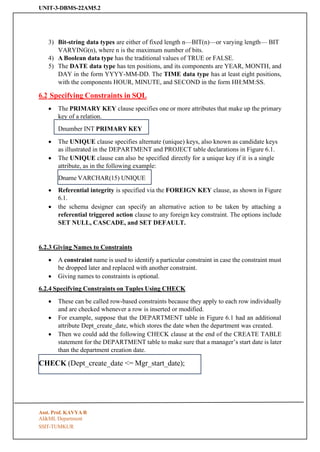
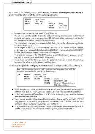
6.2 Specifying Constraints in SQL
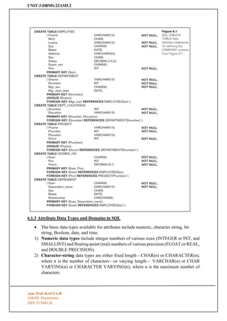
• The PRIMARY KEY clause specifies one or more attributes that make up the primary
key of a relation.
• The UNIQUE clause specifies alternate (unique) keys, also known as candidate keys
as illustrated in the DEPARTMENT and PROJECT table declarations in Figure 6.1.
• The UNIQUE clause can also be specified directly for a unique key if it is a single
attribute, as in the following example:
• Referential integrity is specified via the FOREIGN KEY clause, as shown in Figure
6.1.
• the schema designer can specify an alternative action to be taken by attaching a
referential triggered action clause to any foreign key constraint. The options include
SET NULL, CASCADE, and SET DEFAULT.
6.2.3 Giving Names to Constraints
• A constraint name is used to identify a particular constraint in case the constraint must
be dropped later and replaced with another constraint.
• Giving names to constraints is optional.
6.2.4 Specifying Constraints on Tuples Using CHECK
• These can be called row-based constraints because they apply to each row individually
and are checked whenever a row is inserted or modified.
• For example, suppose that the DEPARTMENT table in Figure 6.1 had an additional
attribute Dept_create_date, which stores the date when the department was created.
• Then we could add the following CHECK clause at the end of the CREATE TABLE
statement for the DEPARTMENT table to make sure that a manager’s start date is later
than the department creation date.
Asst. Prof. KAVYA R
AI&ML Department
Dname VARCHAR(15) UNIQUE
Dnumber INT PRIMARY KEY

4. UNIT-3-DBMS-22AM5.2
SSIT-TUMKUR
• The CHECK clause can also be used to specify more general constraints using the
CREATE ASSERTION statement of SQL.
6.3 Basic Retrieval Queries in SQL
The basic form of the SELECT statement, sometimes called a mapping or a
select-from-where block, is formed of the three clauses SELECT, FROM, and
WHERE and has the following form:
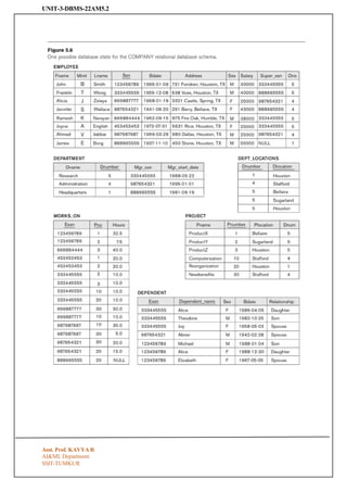
SCHEMA DIAGRAM OF COMPANY DATABASE
Asst. Prof. KAVYA R
AI&ML Department

5. UNIT-3-DBMS-22AM5.2
SSIT-TUMKUR
Asst. Prof. KAVYA R
AI&ML Department

6. UNIT-3-DBMS-22AM5.2
SSIT-TUMKUR
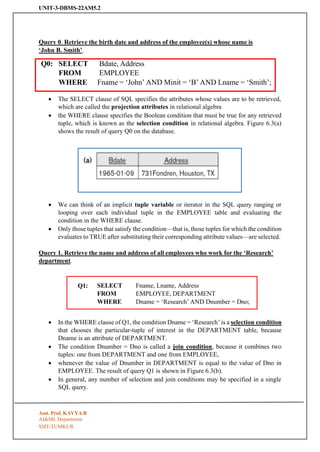
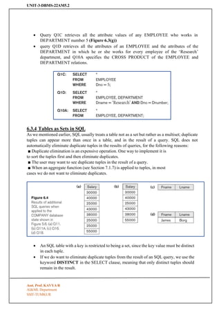
Query 0. Retrieve the birth date and address of the employee(s) whose name is
‘John B. Smith’.
Q0: SELECT
FROM
Bdate, Address
EMPLOYEE
WHERE Fname = ‘John’ AND Minit = ‘B’ AND Lname = ‘Smith’;
• The SELECT clause of SQL specifies the attributes whose values are to be retrieved,
which are called the projection attributes in relational algebra
• the WHERE clause specifies the Boolean condition that must be true for any retrieved
tuple, which is known as the selection condition in relational algebra. Figure 6.3(a)
shows the result of query Q0 on the database.
• We can think of an implicit tuple variable or iterator in the SQL query ranging or
looping over each individual tuple in the EMPLOYEE table and evaluating the
condition in the WHERE clause.
• Only those tuples that satisfy the condition—that is, those tuples for which the condition
evaluates to TRUE after substituting their corresponding attribute values—are selected.
Query 1. Retrieve the name and address of all employees who work for the ‘Research’
department.
Q1: SELECT
FROM
Fname, Lname, Address
EMPLOYEE, DEPARTMENT
WHERE Dname = ‘Research’ AND Dnumber = Dno;
• In the WHERE clause of Q1, the condition Dname = ‘Research’ is a selection condition
that chooses the particular-tuple of interest in the DEPARTMENT table, because
Dname is an attribute of DEPARTMENT.
• The condition Dnumber = Dno is called a join condition, because it combines two
tuples: one from DEPARTMENT and one from EMPLOYEE,
• whenever the value of Dnumber in DEPARTMENT is equal to the value of Dno in
EMPLOYEE. The result of query Q1 is shown in Figure 6.3(b).
• In general, any number of selection and join conditions may be specified in a single
SQL query.
Asst. Prof. KAVYA R
AI&ML Department

7. UNIT-3-DBMS-22AM5.2
SSIT-TUMKUR
• A query that involves only selection and join conditions plus projection attributes is
known as a select-project-join query.
• The next example is a select-project-join query with two join conditions
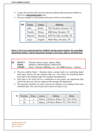
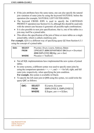
Query 2. For every project located in ‘Stafford’, list the project number, the controlling
department number, and the department manager’s last name, address, and birth date.
Q2: SELECT
FROM
Pnumber, Dnum, Lname, Address, Bdate
PROJECT, DEPARTMENT, EMPLOYEE
WHERE Dnum = Dnumber AND Mgr_ssn = Ssn AND Plocation = ‘Stafford.
• The join condition Dnum = Dnumber relates a project tuple to its controlling depart
ment tuple, whereas the join condition Mgr_ssn = Ssn relates the controlling depart
ment tuple to the employee tuple who manages that department.
• Each tuple in the result will be a combination of one project, one department (that
controls the proj ect), and one employee (that manages the department).
• The projection attributes are used to choose the attributes to be displayed from each
combined tuple. The result of query Q2 is shown in Figure 6.3(c).
Asst. Prof. KAVYA R
AI&ML Department

8. UNIT-3-DBMS-22AM5.2
SSIT-TUMKUR
Q1A: SELECT
FROM
WHERE
Fname, EMPLOYEE.Name, Address
EMPLOYEE, DEPARTMENT
DEPARTMENT.Name = ‘Research’ AND
DEPARTMENT.Dnumber = EMPLOYEE.Dnumber;
Q1′: SELECT
FROM
WHERE
EMPLOYEE.Fname, EMPLOYEE.LName, EMPLOYEE.Address
EMPLOYEE, DEPARTMENT
DEPARTMENT.DName = ‘Research’ AND
DEPARTMENT.Dnumber = EMPLOYEE.Dno;
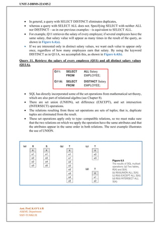
6.3.2 Ambiguous Attribute Names, Aliasing, Renaming, and Tuple Variables
• In SQL, the same name can be used for two (or more) attributes as long as the attributes are
in different tables.
• If this is the case, and a multitable query refers to two or more attributes with the same name,
we must qualify the attribute name with the relation name to prevent ambiguity.
• This is done by prefixing the relation’s name to the attribute name and separating the two by
a period. To illustrate this, suppose that in Figures 5.5 and 5.6
• the Dno and Lname attributes of the EMPLOYEE relation were called Dnumber and
Name, and the Dname attribute of DEPARTMENT was also called Name; then, to prevent
ambiguity,
• Query Q1 would be rephrased as shown in Q1A. We must prefix the attributes Name and
Dnumber in Q1A to specify which ones we are referring to, because the same attribute names
are used in both relations:
• Fully qualified attribute names can be used for clarity even if there is no ambiguity in attribute
names. Q1 can be rewritten as Q1′ below with fully qualified attribute names.
• We can also rename the table names to shorter names by creating an alias for each table name
to avoid repeated typing of long table names (see Q8 below).
• The ambiguity of attribute names also arises in the case of queries that refer to the same
relation twice, as in the following example.
Asst. Prof. KAVYA R
AI&ML Department

9. UNIT-3-DBMS-22AM5.2
SSIT-TUMKUR
EMPLOYEE AS E (Fn, Mi, Ln, Ssn, Bd, Addr, Sex, Sal, Sssn, Dno)
Query 8. For each employee, retrieve the employee’s first and last name and the first and last
name of his or her immediate supervisor.
Q8: SELECT
FROM
E.Fname, E.Lname, S.Fname, S.Lname
EMPLOYEE AS E, EMPLOYEE AS S
WHERE E.Super_ssn = S.Ssn;
• In this case, we are required to declare alternative relation names E and S, called aliases or
tuple variables, for the EMPLOYEE relation.
• An alias can follow the key word AS, as shown in Q8, or it can directly follow the relation
name—for example, by writing EMPLOYEE E, EMPLOYEE S in the FROM clause of Q8.
• It is also possible to rename the relation attributes within the query in SQL by giving them
aliases.
For example, if we write
in the FROM clause, Fn becomes an alias for Fname, Mi for Minit, Ln for Lname, and so on.
• In Q8, we can think of E and S as two different copies of the EMPLOYEE relation;
• the first, E, represents employees in the role of supervisees or subordinates;
• the second, S, represents employees in the role of supervisors.
• We can now join the two copies. Of course, in reality there is only one EMPLOYEE relation,
and the join condition is meant to join the relation with itself by matching the tuples that satisfy
the join condition E.Super_ssn = S.Ssn.
• Notice that this is an example of a one-level recursive query, as we will discuss in Section 8.4.2.
• In earlier versions of SQL, it was not possible to specify a general recursive query, with an
unknown number of levels, in a single SQL statement.
• The result of query Q8 is shown in Figure 6.3(d). Whenever one or more aliases are given to a
relation, we can use these names to represent different references to that same relation.
• This permits multiple references to the same relation within a query.
• We can use this alias-naming or renaming mechanism in any SQL query to specify tuple
variables for every table in the WHERE clause, whether the same relation needs to be
referenced more than once. In fact, this practice is recommended since it results in queries that
are easier to comprehend.
Asst. Prof. KAVYA R
AI&ML Department

10. UNIT-3-DBMS-22AM5.2
SSIT-TUMKUR
Q1B: SELECT
FROM
WHERE
E.Fname, E.LName, E.Address
EMPLOYEE AS E, DEPARTMENT AS D
D.DName = ‘Research’ AND D.Dnumber = E.Dno;
For example, we could specify query Q1 as in Q1B
6.3.3 Unspecified WHERE Clause and Use of the Asterisk
• We discuss two more features of SQL here. A missing WHERE clause indicates no condition
on tuple selection; hence, all tuples of the relation specified in the FROM clause qualify and
are selected for the query result.
• If more than one relation is specified in the FROM clause and there is no WHERE clause, then
the CROSS PRODUCT—all possible tuple combinations—of these relations is selected.
• For example, Query 9 selects all EMPLOYEE Ssns (Figure 6.3(e)), and Query 10 selects all
combinations of an EMPLOYEE Ssn and a DEPARTMENT Dname, regardless of whether the
employee works for the department or not (Figure 6.3(f)).
Asst. Prof. KAVYA R
AI&ML Department

11. UNIT-3-DBMS-22AM5.2
SSIT-TUMKUR
Queries 9 and 10. Select all EMPLOYEE Ssns (Q9) and all combinations of EMPLOYEE
Ssn and DEPARTMENT Dname (Q10) in the database.
Q9: SELECT
FROM
Ssn
EMPLOYEE;
Q10: SELECT Ssn, Dname
FROM EMPLOYEE, DEPARTMENT;
• It is extremely important to specify every selection and join condition in the WHERE
clause; if any such condition is overlooked, incorrect and very large relations may
result.
• Notice that Q10 is similar to a CROSS-PRODUCT operation followed by a
PROJECT operation in relational algebra (see Chapter 8).
• If we specify all the attributes of EMPLOYEE and DEPARTMENT in Q10, we get the
actual CROSS PRODUCT (except for duplicate elimination, if any).
• To retrieve all the attribute values of the selected tuples, we do not have to list the attribute
names explicitly in SQL; we just specify an asterisk (*), which stands for all the
attributes.
• The * can also be prefixed by the relation name or alias; for example, EMPLOYEE.*
refers to all attributes of the EMPLOYEE table.
Asst. Prof. KAVYA R
AI&ML Department

12. UNIT-3-DBMS-22AM5.2
SSIT-TUMKUR
• Query Q1C retrieves all the attribute values of any EMPLOYEE who works in
DEPARTMENT number 5 (Figure 6.3(g))
• query Q1D retrieves all the attributes of an EMPLOYEE and the attributes of the
DEPARTMENT in which he or she works for every employee of the ‘Research’
department, and Q10A specifies the CROSS PRODUCT of the EMPLOYEE and
DEPARTMENT relations.
6.3.4 Tables as Sets in SQL
As we mentioned earlier, SQL usually treats a table not as a set but rather as a multiset; duplicate
tuples can appear more than once in a table, and in the result of a query. SQL does not
automatically eliminate duplicate tuples in the results of queries, for the following reasons:
■ Duplicate elimination is an expensive operation. One way to implement it is
to sort the tuples first and then eliminate duplicates.
■ The user may want to see duplicate tuples in the result of a query.
■ When an aggregate function (see Section 7.1.7) is applied to tuples, in most
cases we do not want to eliminate duplicates.
• An SQL table with a key is restricted to being a set, since the key value must be distinct
in each tuple.
• If we do want to eliminate duplicate tuples from the result of an SQL query, we use the
keyword DISTINCT in the SELECT clause, meaning that only distinct tuples should
remain in the result.
Asst. Prof. KAVYA R
AI&ML Department

13. UNIT-3-DBMS-22AM5.2
SSIT-TUMKUR
• In general, a query with SELECT DISTINCT eliminates duplicates,
• whereas a query with SELECT ALL does not. Specifying SELECT with neither ALL
nor DISTINCT—as in our previous examples—is equivalent to SELECT ALL.
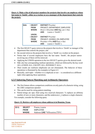
• For example, Q11 retrieves the salary of every employee; if several employees have the
same salary, that salary value will appear as many times in the result of the query, as
shown in Figure 6.4(a).
• If we are interested only in distinct salary values, we want each value to appear only
once, regardless of how many employees earn that salary. By using the keyword
DISTINCT as in Q11A, we accomplish this, as shown in Figure 6.4(b).
Query 11. Retrieve the salary of every employee (Q11) and all distinct salary values
(Q11A).
• SQL has directly incorporated some of the set operations from mathematical set theory,
which are also part of relational algebra (see Chapter 8).
• There are set union (UNION), set difference (EXCEPT), and set intersection
(INTERSECT) operations.
• The relations resulting from these set operations are sets of tuples; that is, duplicate
tuples are eliminated from the result.
• These set operations apply only to type- compatible relations, so we must make sure
that the two relations on which we apply the operation have the same attributes and that
the attributes appear in the same order in both relations. The next example illustrates
the use of UNION.
Asst. Prof. KAVYA R
AI&ML Department

14. UNIT-3-DBMS-22AM5.2
SSIT-TUMKUR
Query 4. Make a list of all project numbers for projects that involve an employee whose
last name is ‘Smith’, either as a worker or as a manager of the department that controls
the project.
• The first SELECT query retrieves the projects that involve a ‘Smith’ as manager of the
department that controls the project, and
• the second retrieves the projects that involve a ‘Smith’ as a worker on the project.
• Notice that if several employees have the last name ‘Smith’, the project names
involving any of them will be retrieved.
• Applying the UNION operation to the two SELECT queries gives the desired result.
• SQL also has corresponding multiset operations, which are followed by the key word
ALL (UNION ALL, EXCEPT ALL, INTERSECT ALL).
• Their results are multisets (duplicates are not eliminated). The behavior of these
operations is illustrated by the examples in Figure 6.5.
• Basically, each tuple—whether it is a duplicate or not— is considered as a different
tuple when applying these operations.
6.3.5 Substring Pattern Matching and Arithmetic Operators
• The first feature allows comparison conditions on only parts of a character string, using
the LIKE comparison operator.
• This can be used for string pattern matching.
• Partial strings are spec ified using two reserved characters: % replaces an arbitrary
number of zero or more characters, and the underscore (_) replaces a single character.
For example, consider the following query
Query 12. Retrieve all employees whose address is in Houston, Texas.
Asst. Prof. KAVYA R
AI&ML Department

15. UNIT-3-DBMS-22AM5.2
SSIT-TUMKUR
• To retrieve all employees who were born during the 1970s, we can use Query Q12A.
• Here, ‘7’ must be the third character of the string (according to our format for date),
• so we use the value ‘_ _ 5 __________ ’, with each underscore serving as a place
holder for an arbitrary character.
Query 12A. Find all employees who were born during the 1950s.
• If an underscore or % is needed as a literal character in the string, the character should be
preceded by an escape character, which is specified after the string using the keyword
ESCAPE.
For example, ‘AB_CD%EF’ ESCAPE ‘’ represents the literal string ‘AB_CD%EF’
because is specified as the escape character.
• Any character not used in the string can be chosen as the escape character.
• we need a rule to specify apostrophes or single quotation marks (‘ ’) if they are to be
included in a string because they are used to begin and end strings.
• If an apostrophe (’) is needed, it is represented as two consecutive apostrophes (”) so that
it will not be interpreted as ending the string.
• Notice that substring comparison implies that attribute values are not atomic (indivisible)
values, as we had assumed in the formal relational model (see Section 5.1) .
• Another feature allows the use of arithmetic in queries.
• The standard arithmetic operators for addition (+), subtraction (−), multiplication (*), and
division (/) can be applied to numeric values or attributes with numeric domains.
For example, suppose that we want to see the effect of giving all employees who work on
the ‘ProductX’ project a 10% raise; we can issue Query 13 to see what their salaries would
become. This example also shows how we can rename an attribute in the query result using
AS in the SELECT clause.
Query 13. Show the resulting salaries if every employee working on the ‘ProductX’ project
is given a 10% raise.
Asst. Prof. KAVYA R
AI&ML Department

16. UNIT-3-DBMS-22AM5.2
SSIT-TUMKUR
• For string data types, the concatenate operator || can be used in a query to append two
string values.
• For date, time, timestamp, and interval data types, operators include incrementing (+)
or decrementing (−) a date, time, or timestamp by an interval.
• In addition, an interval value is the result of the difference between two date, time, or
timestamp values.
• Another comparison operator, which can be used for convenience, is BETWEEN,
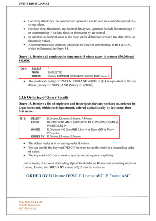
which is illustrated in Query 14.
Query 14. Retrieve all employees in department 5 whose salary is between $30,000 and
$40,000.
• The condition (Salary BETWEEN 30000 AND 40000) in Q14 is equivalent to the con
dition ((Salary >= 30000) AND (Salary <= 40000)).
6.3.6 Ordering of Query Results
Query 15. Retrieve a list of employees and the projects they are working on, ordered by
department and, within each department, ordered alphabetically by last name, then
first name.
• The default order is in ascending order of values.
• We can specify the keyword DESC if we want to see the result in a descending order
of values.
• The keyword ASC can be used to specify ascending order explicitly.
For example, if we want descending alphabetical order on Dname and ascending order on
Lname, Fname, the ORDER BY clause of Q15 can be written as
ORDER BY D.Dname DESC, E.Lname ASC, E.Fname ASC
Asst. Prof. KAVYA R
AI&ML Department

17. UNIT-3-DBMS-22AM5.2
SSIT-TUMKUR
6.3.7 Discussion and Summary of Basic SQL Retrieval Querie
• A simple retrieval query in SQL can consist of up to four clauses, but only the first
two SELECT and FROM—are mandatory.
• The clauses are specified in the following order, with the clauses between square
brackets [ … ] being optional:
• The SELECT clause lists the attributes to be retrieved,
• FROM clause specifies all relations (tables) needed in the simple query.
• WHERE clause identifies the conditions for selecting the tuples from these relations,
including join conditions if needed.
• ORDER BY specifies an order for displaying the results of a query.
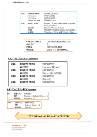
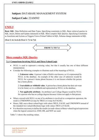
6.4 INSERT, DELETE, and UPDATE Statements in SQL
6.4.1 The INSERT Command
Asst. Prof. KAVYA R
AI&ML Department

18. UNIT-3-DBMS-22AM5.2
SSIT-TUMKUR
TXT BOOK-1: 6.1 TO 6.4 COMPLETED
6.4.2 The DELETE Command
6.4.3 The UPDATE Command
Asst. Prof. KAVYA R
AI&ML Department

19. UNIT-3-DBMS-22AM5.2
Asst. Prof. KAVYA R
AI&ML Department
SSIT-TUMKUR
FROM 7.1 TO 7.4
Subject: DATABASE MANAGEMENT SYSTEM
Subject Code: 22AM502
UNIT-3
Basic SQL: Data Definition and Data Types, Specifying constraints in SQL, Basic retrieval queries in
SQL, Insert, Delete and Update statements in SQL. More complex SQL Queries, Specifying Constraints
as Assertions and Actions as Triggers Views (Virtual Tables) in SQL, Schema change statements in SQL.
(Text 1: 6.1 to 6.4) (Text 1: 7.1 to 7.4)
More complex SQL Queries
7.1.1 Comparisons Involving NULL and Three-Valued Logic
• NULL is used to represent a missing value, but that it usually has one of three different
interpretations
• Consider the following examples to illustrate each of the meanings of NULL.
1. Unknown value. A person’s date of birth is not known, so it is represented by
NULL in the database. An example of the other case of unknown would be
NULL for a person’s home phone because it is not known whether the person
has a home phone.
2. Unavailable or withheld value. A person has a home phone but does not want
it to be listed, so it is withheld and represented as NULL in the database.
3. Not applicable attribute. An attribute Last College Degree would be NULL
for a person who has no college degrees because it does not apply to that person.
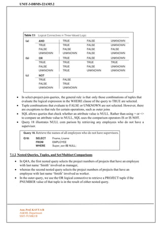
• When a record with NULL in one of its attributes is involved in a comparison operation, the
result is UNKNOWN (it may be TRUE or it may be FALSE).
• Hence, SQL uses a three-valued logic with values TRUE, FALSE, and UNKNOWN instead of
the standard two-valued (Boolean) logic with values TRUE or FALSE.
• It is therefore necessary to define the results (or truth values) of three-valued logical expressions
when the logical connectives AND, OR, and NOT are used.
Table 7.1 shows the resulting values.

20. UNIT-3-DBMS-22AM5.2
Asst. Prof. KAVYA R
AI&ML Department
SSIT-TUMKUR
• In select-project-join queries, the general rule is that only those combinations of tuples that
evaluate the logical expression in the WHERE clause of the query to TRUE are selected.
• Tuple combinations that evaluate to FALSE or UNKNOWN are not selected. However, there
are exceptions to that rule for certain operations, such as outer joins
• SQL allows queries that check whether an attribute value is NULL. Rather than using = or <>
to compare an attribute value to NULL, SQL uses the comparison operators IS or IS NOT.
• Query 18 illustrates NULL com parison by retrieving any employees who do not have a
supervisor.
7.1.2 Nested Queries, Tuples, and Set/Multiset Comparisons
• In Q4A, the first nested query selects the project numbers of projects that have an employee
with last name ‘Smith’ involved as manager,
• whereas the second nested query selects the project numbers of projects that have an
employee with last name ‘Smith’ involved as worker.
• In the outer query, we use the OR logical connective to retrieve a PROJECT tuple if the
PNUMBER value of that tuple is in the result of either nested query.

21. UNIT-3-DBMS-22AM5.2
Asst. Prof. KAVYA R
AI&ML Department
SSIT-TUMKUR
• If a nested query returns a single attribute and a single tuple, the query result will be a single
(scalar) value.
• In such cases, it is permissible to use = instead of IN for the comparison operator.
• In general, the nested query will return a table (relation), which is a set or multiset of tuples.
SQL allows the use of tuples of values in comparisons by placing them within parentheses.
To illustrate this, consider the following query:
• This query will select the Essns of all employees who work the same (project, hours)
combination on some project that employee ‘John Smith’ (whose Ssn = ‘123456789’)
works on.
• In this example, the IN operator compares the subtuple of values in paren theses (Pno,
Hours) within each tuple in WORKS_ON with the set of type-compatible tuples produced
by the nested query.
• In addition to the IN operator, several other comparison operators can be used to compare
a single value v (typically an attribute name) to a set or multiset v (typically a nested query).
• The = ANY (or = SOME) operator returns TRUE if the value v is equal to some value in
the set V and is hence equivalent to IN.
• The two keywords ANY and SOME have the same effect. Other operators that can be
combined with ANY (or SOME) include >, >=, <=, and <>.
• The keyword ALL can also be com bined with each of these operators.
• For example, the comparison condition (v > ALL V) returns TRUE if the value v is greater
than all the values in the set (or multiset) V.

22. UNIT-3-DBMS-22AM5.2
Asst. Prof. KAVYA R
AI&ML Department
SSIT-TUMKUR
An example is the following query, which returns the names of employees whose salary is
greater than the salary of all the employees in department 5:
• In general, we can have several levels of nested queries.
• We can once again be faced with possible ambiguity among attribute names if attributes of
the same name exist—one in a relation in the FROM clause of the outer query, and another
in a relation in the FROM clause of the nested query.
• The rule is that a reference to an unqualified attribute refers to the relation declared in the
innermost nested query.
For example, in the SELECT clause and WHERE clause of the first nested query of Q4A,
a reference to any unqualified attribute of the PROJECT relation refers to the PROJECT
relation specified in the FROM clause of the nested query.
• To refer to an attribute of the PROJECT relation specified in the outer query, we specify
and refer to an alias (tuple variable) for that relation.
• These rules are similar to scope rules for program variables in most programming
languages that allow nested procedures and functions.
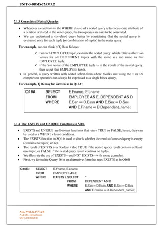
To illustrate the potential ambiguity of attribute names in nested queries, consider Query 16.
• In the nested query of Q16, we must qualify E.Sex because it refers to the Sex attribute of
EMPLOYEE from the outer query, and DEPENDENT also has an attribute called Sex.
• If there were any unqualified references to Sex in the nested query, they would refer to the
Sex attribute of DEPENDENT.
• However, we would not have to qualify the attributes Fname and Ssn of EMPLOYEE if
they appeared in the nested query because the DEPENDENT relation does not have
attributes called Fname and Ssn, so there is no ambiguity.
• It is generally advisable to create tuple variables (aliases) for all the tables referenced in
an SQL query to avoid potential errors and ambiguities, as illustrated in Q16.

23. UNIT-3-DBMS-22AM5.2
Asst. Prof. KAVYA R
AI&ML Department
SSIT-TUMKUR
7.1.3 Correlated Nested Queries
• Whenever a condition in the WHERE clause of a nested query references some attribute of
a relation declared in the outer query, the two queries are said to be correlated.
• We can understand a correlated query better by considering that the nested query is
evaluated once for each tuple (or combination of tuples) in the outer query.
For example, we can think of Q16 as follows:
✓ For each EMPLOYEE tuple, evaluate the nested query, which retrieves the Essn
values for all DEPENDENT tuples with the same sex and name as that
EMPLOYEE tuple;
✓ if the Ssn value of the EMPLOYEE tuple is in the result of the nested query,
then select that EMPLOYEE tuple.
• In general, a query written with nested select-from-where blocks and using the = or IN
comparison operators can always be expressed as a single block query.
For example, Q16 may be written as in Q16A:
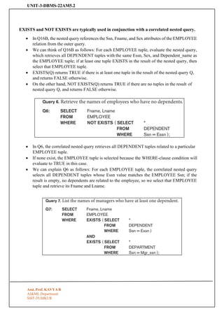
7.1.4 The EXISTS and UNIQUE Functions in SQL
• EXISTS and UNIQUE are Boolean functions that return TRUE or FALSE; hence, they can
be used in a WHERE clause condition.
• The EXISTS function in SQL is used to check whether the result of a nested query is empty
(contains no tuples) or not.
• The result of EXISTS is a Boolean value TRUE if the nested query result contains at least
one tuple, or FALSE if the nested query result contains no tuples.
• We illustrate the use of EXISTS—and NOT EXISTS—with some examples.
• First, we formulate Query 16 in an alternative form that uses EXISTS as in Q16B

24. UNIT-3-DBMS-22AM5.2
Asst. Prof. KAVYA R
AI&ML Department
SSIT-TUMKUR
EXISTS and NOT EXISTS are typically used in conjunction with a correlated nested query.
• In Q16B, the nested query references the Ssn, Fname, and Sex attributes of the EMPLOYEE
relation from the outer query.
• We can think of Q16B as follows: For each EMPLOYEE tuple, evaluate the nested query,
which retrieves all DEPENDENT tuples with the same Essn, Sex, and Dependent_name as
the EMPLOYEE tuple; if at least one tuple EXISTS in the result of the nested query, then
select that EMPLOYEE tuple.
• EXISTS(Q) returns TRUE if there is at least one tuple in the result of the nested query Q,
and returns FALSE otherwise.
• On the other hand, NOT EXISTS(Q) returns TRUE if there are no tuples in the result of
nested query Q, and returns FALSE otherwise.
• In Q6, the correlated nested query retrieves all DEPENDENT tuples related to a particular
EMPLOYEE tuple.
• If none exist, the EMPLOYEE tuple is selected because the WHERE-clause condition will
evaluate to TRUE in this case.
• We can explain Q6 as follows: For each EMPLOYEE tuple, the correlated nested query
selects all DEPENDENT tuples whose Essn value matches the EMPLOYEE Ssn; if the
result is empty, no dependents are related to the employee, so we select that EMPLOYEE
tuple and retrieve its Fname and Lname.

25. UNIT-3-DBMS-22AM5.2
Asst. Prof. KAVYA R
AI&ML Department
SSIT-TUMKUR
• One way to write this query is shown in Q7, where we specify two nested correlated
queries;
• the first selects all DEPENDENT tuples related to an EMPLOYEE, and the second selects
all DEPARTMENT tuples managed by the EMPLOYEE.
• If at least one of the first and at least one of the second exists, we select the EMPLOYEE
tuple.
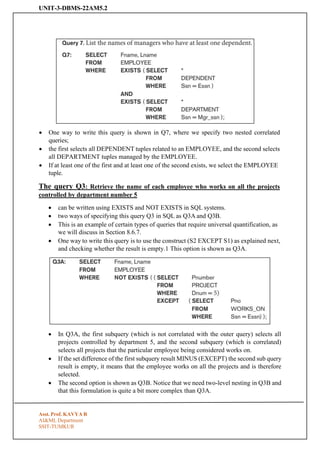
The query Q3: Retrieve the name of each employee who works on all the projects
controlled by department number 5
• can be written using EXISTS and NOT EXISTS in SQL systems.
• two ways of specifying this query Q3 in SQL as Q3A and Q3B.
• This is an example of certain types of queries that require universal quantification, as
we will discuss in Section 8.6.7.
• One way to write this query is to use the construct (S2 EXCEPT S1) as explained next,
and checking whether the result is empty.1 This option is shown as Q3A.
• In Q3A, the first subquery (which is not correlated with the outer query) selects all
projects controlled by department 5, and the second subquery (which is correlated)
selects all projects that the particular employee being considered works on.
• If the set difference of the first subquery result MINUS (EXCEPT) the second sub query
result is empty, it means that the employee works on all the projects and is therefore
selected.
• The second option is shown as Q3B. Notice that we need two-level nesting in Q3B and
that this formulation is quite a bit more complex than Q3A.

26. UNIT-3-DBMS-22AM5.2
Asst. Prof. KAVYA R
AI&ML Department
SSIT-TUMKUR
• In Q3B, the outer nested query selects any WORKS_ON (B) tuples whose Pno is of a
project controlled by department 5, if there is not a WORKS_ON (C) tuple with the
same Pno and the same Ssn as that of the EMPLOYEE tuple under consideration in the
outer query.
• If no such tuple exists, we select the EMPLOYEE tuple.
• The form of Q3B matches the following rephrasing of Query 3: Select each
employee such that there does not exist a project controlled by department 5 that
the employee does not work on.
• It corresponds to the way we will write this query in tuple relation calculus (see Section
8.6.7).
• There is another SQL function, UNIQUE(Q), which returns TRUE if there are no
duplicate tuples in the result of query Q; otherwise, it returns FALSE.
• This can be used to test whether the result of a nested query is a set (no duplicates) or
a multiset (duplicates exist).
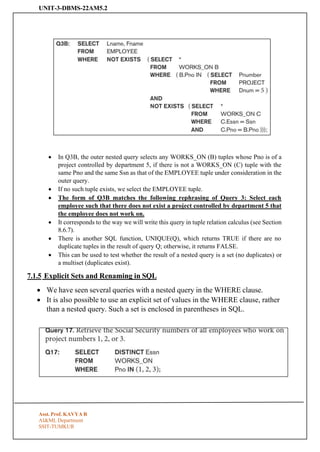
7.1.5 Explicit Sets and Renaming in SQL
• We have seen several queries with a nested query in the WHERE clause.
• It is also possible to use an explicit set of values in the WHERE clause, rather
than a nested query. Such a set is enclosed in parentheses in SQL.

27. UNIT-3-DBMS-22AM5.2
Asst. Prof. KAVYA R
AI&ML Department
SSIT-TUMKUR
• In SQL, it is possible to rename any attribute that appears in the result of a
query by adding the qualifier AS followed by the desired new name.
• Hence, the AS construct can be used to alias both attribute and relation
names in general, and it can be used in appropriate parts of a query.
For example, Q8A shows how query Q8 from Section 4.3.2 can be slightly
changed to retrieve the last name of each employee and his or her supervisor
while renaming the resulting attribute names as Employee_name and
Supervisor_name.
✓ The new names will appear as column headers for the query result.
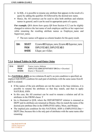
7.1.6 Joined Tables in SQL and Outer Joins
In a NATURAL JOIN on two relations R and S, no join condition is specified; an
implicit EQUIJOIN condition for each pair of attributes with the same name from R
and S is created.
• If the names of the join attributes are not the same in the base relations, it is
possible to rename the attributes so that they match, and then to apply
NATURAL JOIN.
• In this case, the AS construct can be used to rename a relation and all its
attributes in the FROM clause. T
• his is illustrated in Q1B, where the DEPARTMENT relation is renamed as
DEPT and its attributes are renamed as Dname, Dno (to match the name of the
desired join attribute Dno in the EMPLOYEE table), Mssn, and Msdate.
• The implied join condition for this NATURAL JOIN is EMPLOYEE.Dno =
DEPT.Dno, because this is the only pair of attributes with the same name after
renaming:

28. UNIT-3-DBMS-22AM5.2
Asst. Prof. KAVYA R
AI&ML Department
SSIT-TUMKUR
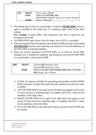
• The default type of join in a joined table is called an INNER JOIN, where a
tuple is included in the result only if a matching tuple exists in the other
relation.
For example, in query Q8A, only employees who have a supervisor are
included in the result;
• An EMPLOYEE tuple whose value for Super_ssn is NULL is excluded.
• If the user requires that all employees be included, a different type of join called
OUTER JOIN must be used explicitly (see Section 8.4.4 for the definition of
OUTER JOIN in relational algebra).
• There are several variations of OUTER JOIN, as we shall see. In the SQL
standard, this is handled by explicitly specifying the keyword OUTER JOIN
in a joined table, as illustrated in Q8B:
• In SQL, the options available for specifying joined tables include INNER
JOIN (only pairs of tuples that match the join condition are retrieved, same
as JOIN),
• LEFT OUTER JOIN (every tuple in the left table must appear in the result;
if it does not have a matching tuple, it is padded with NULL values for the
attributes of the right table),
• RIGHT OUTER JOIN (every tuple in the right table must appear in the
result; if it does not have a matching tuple, it is padded with NULL values
for the attributes of the left table),
• FULL OUTER JOIN. In the latter three options, the keyword OUTER may
be omitted.

29. UNIT-3-DBMS-22AM5.2
Asst. Prof. KAVYA R
AI&ML Department
SSIT-TUMKUR
• If the join attributes have the same name, one can also specify the natural
join variation of outer joins by using the keyword NATURAL before the
operation (for example, NATURAL LEFT OUTER JOIN).
• The keyword CROSS JOIN is used to specify the CARTESIAN
PRODUCT operation (see Section 8.2.2), although this should be used only
with the utmost care because it generates all possible tuple combinations.
• It is also possible to nest join specifications; that is, one of the tables in a
join may itself be a joined table.
• This allows the specification of the join of three or more tables as a single
joined table, which is called a multiway join.
For example, Q2A is a different way of specifying query Q2 from Section 6.3.1
using the concept of a joined table:
• Not all SQL implementations have implemented the new syntax of joined
tables.
• In some systems, a different syntax was used to specify outer joins by
using the comparison operators + =, = +, and + = + for left, right, and full
outer join, respectively, when specifying the join condition.
For example, this syntax is available in Oracle.
• To specify the left outer join in Q8B using this syntax, we could write the
query Q8C as follows:

30. UNIT-3-DBMS-22AM5.2
Asst. Prof. KAVYA R
AI&ML Department
SSIT-TUMKUR
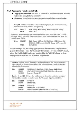
7.1.7 Aggregate Functions in SQL
• Aggregate functions are used to summarize information from multiple
tuples into a single-tuple summary.
• Grouping is used to create subgroups of tuples before summarization.
If we want to get the preceding aggregate function values for employees of a
specific department—say, the ‘Research’ department—we can write Query 20,
where the EMPLOYEE tuples are restricted by the WHERE clause to those
employees who work for the ‘Research’ department.

31. UNIT-3-DBMS-22AM5.2
Asst. Prof. KAVYA R
AI&ML Department
SSIT-TUMKUR
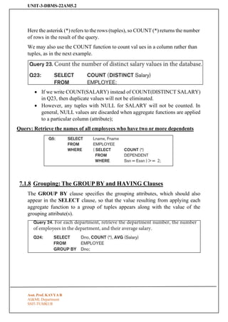
Here the asterisk (*) refers to the rows (tuples), so COUNT (*) returns the number
of rows in the result of the query.
We may also use the COUNT function to count val ues in a column rather than
tuples, as in the next example.
• If we write COUNT(SALARY) instead of COUNT(DISTINCT SALARY)
in Q23, then duplicate values will not be eliminated.
• However, any tuples with NULL for SALARY will not be counted. In
general, NULL values are discarded when aggregate functions are applied
to a particular column (attribute);
Query: Retrieve the names of all employees who have two or more dependents
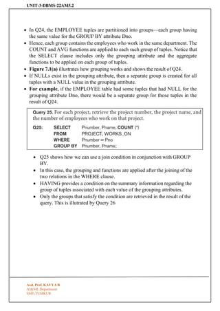
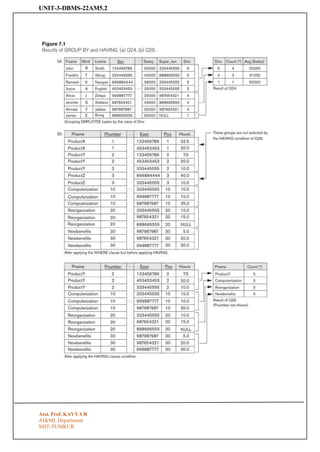
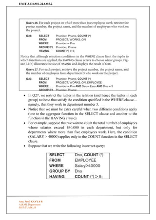
7.1.8 Grouping: The GROUP BY and HAVING Clauses
The GROUP BY clause specifies the grouping attributes, which should also
appear in the SELECT clause, so that the value resulting from applying each
aggregate function to a group of tuples appears along with the value of the
grouping attribute(s).

32. UNIT-3-DBMS-22AM5.2
Asst. Prof. KAVYA R
AI&ML Department
SSIT-TUMKUR
• In Q24, the EMPLOYEE tuples are partitioned into groups—each group having
the same value for the GROUP BY attribute Dno.
• Hence, each group contains the employees who work in the same department. The
COUNT and AVG functions are applied to each such group of tuples. Notice that
the SELECT clause includes only the grouping attribute and the aggregate
functions to be applied on each group of tuples.
• Figure 7.1(a) illustrates how grouping works and shows the result of Q24.
• If NULLs exist in the grouping attribute, then a separate group is created for all
tuples with a NULL value in the grouping attribute.
• For example, if the EMPLOYEE table had some tuples that had NULL for the
grouping attribute Dno, there would be a separate group for those tuples in the
result of Q24.
• Q25 shows how we can use a join condition in conjunction with GROUP
BY.
• In this case, the grouping and functions are applied after the joining of the
two relations in the WHERE clause.
• HAVING provides a condition on the summary information regarding the
group of tuples associated with each value of the grouping attributes.
• Only the groups that satisfy the condition are retrieved in the result of the
query. This is illutrated by Query 26

33. UNIT-3-DBMS-22AM5.2
Asst. Prof. KAVYA R
AI&ML Department
SSIT-TUMKUR

34. UNIT-3-DBMS-22AM5.2
Asst. Prof. KAVYA R
AI&ML Department
SSIT-TUMKUR
• In Q27, we restrict the tuples in the relation (and hence the tuples in each
group) to those that satisfy the condition specified in the WHERE clause—
namely, that they work in department number 5.
• Notice that we must be extra careful when two different conditions apply
(one to the aggregate function in the SELECT clause and another to the
function in the HAVING clause).
• For example, suppose that we want to count the total number of employees
whose salaries exceed $40,000 in each department, but only for
departments where more than five employees work. Here, the condition
(SALARY > 40000) applies only to the COUNT function in the SELECT
clause.
• Suppose that we write the following incorrect query:

35. UNIT-3-DBMS-22AM5.2
Asst. Prof. KAVYA R
AI&ML Department
SSIT-TUMKUR
This is incorrect because it will select only departments that have more than five
employees who each earn more than $40,000.
The rule is that the WHERE clause is executed first, to select individual tuples or
joined tuples; the HAVING clause is applied later, to select individual groups of
tuples.
In the incorrect query, the tuples are already restricted to employees who earn
more than $40,000 before the function in the HAVING clause is applied.
One way to write this query correctly is to use a nested query, as shown in Query
28.

36. 7.1.9 Other SQL Constructs: WITH and CASE:
• SQL also has a CASE construct, which can be used when a value can be different based
on certain conditions.
• This can be used in any part of an SQL query where a value is expected, including when
querying, inserting, or updating tuples. We illustrate this with an example.
7.1.10 Recursive Queries in SQL:
• An example of a recursive relationship between tuples of the same type is the
relationship between an employee and a supervisor.
• An example of a recursive operation is to retrieve all supervisees of a supervisory
employee e at all levels—that is, all employees e′ directly supervised by e, all
employees e′ directly supervised by each employee e′, all employees e″′ directly
supervised by each employee e″, and so on. In SQL:99, this query can be written as
follows:
7.1.11 Discussion and Summary of SQL Queries
• A retrieval query in SQL can consist of up to six clauses, but only the first two—
SELECT and FROM—are mandatory. The query can span several lines, and is ended
by a semicolon.
• Query terms are separated by spaces, and parentheses can be used to group relevant
parts of a query in the standard way.
• The clauses are specified in the following order, with the clauses between square
brackets [ … ] being optional:

37. 7.2 Specifying Constraints as Assertions and Actions as Triggers
• CREATE ASSERTION, which can be used to specify additional types of constraints
that are outside the scope of the built-in relational model constraints (primary and
unique keys, entity integrity, and referential integrity).
• These built-in constraints can be specified within the CREATE TABLE statement of
SQL.
• CREATE TRIGGER, which can be used to specify automatic actions that the database
system will perform when certain events and conditions occur. This type of
functionality is generally referred to as active databases.
7.2.1 Specifying General Constraints as Assertions in SQL
In SQL, users can specify general constraints—those that do not fall into any of the categories
For example, to specify the constraint that
Query: the salary of an employee must not be greater than the salary of the manager of the
department that the employee works for in SQL,
7.2.2 Introduction to Triggers in SQL
• Another important statement in SQL is CREATE TRIGGER. In many cases it is
convenient to specify the type of action to be taken when certain events occur and
when certain conditions are satisfied.
• Suppose we want to check whenever an employee’s salary is greater than the salary of
his or her direct supervisor in the COMPANY database (see Figures 5.5 and 5.6).
• Several events can trigger this rule: inserting a new employee record, changing an
employee’s salary, or changing an employee’s supervisor.
• Suppose that the action to take would be to call an external stored procedure
SALARY_VIOLATION,5 which will notify the supervisor.

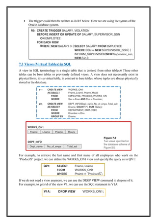
38. • The trigger could then be written as in R5 below. Here we are using the syntax of the
Oracle database system.
7.3 Views (Virtual Tables) in SQL
A view in SQL terminology is a single table that is derived from other tables.6 These other
tables can be base tables or previously defined views. A view does not necessarily exist in
physical form; it is a virtual table, in contrast to base tables, whose tuples are always physically
stored in the database.
For example, to retrieve the last name and first name of all employees who work on the
‘ProductX’ project, we can utilize the WORKS_ON1 view and specify the query as in QV1:
If we do not need a view anymore, we can use the DROP VIEW command to dispose of it.
For example, to get rid of the view V1, we can use the SQL statement in V1A:

39. 7.3.3 View Implementation, View Update, and Inline Views
• query modification, involves modifying or transforming the view query (submitted by the
user) into a query on the underlying base tables. For example, the query QV1 would be
automatically modified to the following query by the DBMS: [COMPLTED ABOVE]
• incremental update -where the DBMS can determine what new tuples must be inserted,
deleted, or modified in a materialized view table when a database update is applied to one of
the defining base tables.
• The view is generally kept as a materialized (physically stored) table as long as it is being
queried.
• If the view is not queried for a certain period of time, the system may then automatically
remove the physical table and recompute it from scratch when future queries reference the
view.
Different strategies as to when a materialized view is updated are possible.
1) The immediate update strategy updates a view as soon as the base tables are changed;
2) the lazy update strategy updates the view when needed by a view query; and the
3) periodic update strategy updates the view periodically (in the latter strategy, a view query may
get a result that is not up-to-date).
7.3.4 Views as Authorization Mechanism
We describe SQL query authorization statements (GRANT and REVOKE).
Suppose a certain user is only allowed to see employee information for employees who
work for department 5;
then we can create the following view DEPT5EMP and grant the user the privilege to query
the view but not the base table EMPLOYEE itself. This user will only be able to retrieve

40. ALTER TABLE COMPANY.EMPLOYEE DROP COLUMN Address CASCADE;
employee information for employee tuples whose Dno = 5, and will not be able to see other
employee tuples when the view is queried.
7.4 Schema Change Statements in SQL
7.4.1 The DROP Command
The DROP command can be used to drop named schema elements, such as tables, domains,
types, or constraints
7.4.2 The ALTER Command
The definition of a base table or of other named schema elements can be changed by using
the ALTER command.
For example,
Add an attribute for keeping track of jobs of employees to the EMPLOYEE base relation in
the COMPANY schema
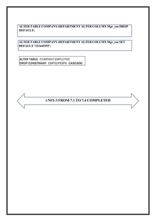
To drop a column, we must choose either CASCADE or RESTRICT for drop behavior.
• If CASCADE is chosen, all constraints and views that reference the column are
dropped automatically from the schema, along with the column.
• If RESTRICT is chosen, the command is successful only if no views or constraints
reference the column.
For example, the following command removes the attribute Address from the EMPLOYEE
base table:
• It is also possible to alter a column definition by dropping an existing default clause
or by defining a new default clause.
The following examples illustrate this clause:

41. ALTER TABLE COMPANY.DEPARTMENT ALTER COLUMN Mgr_ssn SET
DEFAULT ‘333445555’;
UNIT-3 FROM 7.1 TO 7.4 COMPLETED
ALTER TABLE COMPANY.DEPARTMENT ALTER COLUMN Mgr_ssn DROP
DEFAULT;