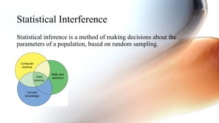
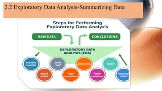
The document presents an overview of data science focusing on statistical inference and exploratory data analysis (EDA), emphasizing their importance in understanding data characteristics, patterns, and relationships. Key aspects of EDA include data distribution analysis, outlier detection, correlation analysis, and handling missing values, often employing Python libraries like Pandas and Matplotlib. The document outlines systematic steps for conducting EDA, including data inspection, transformation, visualization, and effective communication of insights.

1. Data Science
Statistical Interference and Exploratory Data Analysis
Presented by Prof. Priyanka Jadhav

2. Preview
• 2.1 Introduction-Population and samples, Data Preparation,
• 2.2 Exploratory Data Analysis-Summarizing Data
• 2.3 Data Distribution, Outlier Treatment, Measuring Symmetry,
Continuous Distribution, Kernel Density, Estimation: Sample and
Estimated Mean, Variance and Standard Scores, Covariance, and
Pearson’s and Spearman’s Rank Correlation

6. Statistical Interference
Statistical inference is a method of making decisions about the
parameters of a population, based on random sampling.

7. Exploratory Data Analysis (EDA)?
• Exploratory Data Analysis (EDA) is a crucial initial step in data science
projects.
• It involves analyzing and visualizing data to understand its key
characteristics, uncover patterns, and identify relationships between
variables refers to the method of studying and exploring record sets to
apprehend their predominant traits, discover patterns, locate outliers,
and identify relationships between variables.
• EDA is normally carried out as a preliminary step before undertaking
extra formal statistical analyses or modeling.

8. Key aspects of EDA include:
•Distribution of Data: Examining the distribution of data points to understand their range,
central tendencies (mean, median), and dispersion (variance, standard deviation).
•Graphical Representations: Utilizing charts such as histograms, box plots, scatter plots, and
bar charts to visualize relationships within the data and distributions of variables.
•Outlier Detection: Identifying unusual values that deviate from other data points. Outliers can
influence statistical analyses and might indicate data entry errors or unique cases.
•Correlation Analysis: Checking the relationships between variables to understand how they
might affect each other. This includes computing correlation coefficients and creating
correlation matrices.
•Handling Missing Values: Detecting and deciding how to address missing data points,
whether by imputation or removal, depending on their impact and the amount of missing data.
•Summary Statistics: Calculating key statistics that provide insight into data trends.
•Testing Assumptions: Many statistical tests and models assume the data meet certain
conditions. EDA helps verify these assumptions.

9. Tools for Performing Exploratory Data Analysis
• Python Libraries
• Pandas: Provides extensive functions for data manipulation and analysis,
including data structure handling and time series functionality.
• Matplotlib: A plotting library for creating static, interactive, and
animated visualizations in Python.
• Seaborn: Built on top of Matplotlib, it provides a high-level interface for
drawing attractive and informative statistical graphics.
• Plotly: An interactive graphing library for making interactive plots and
offers more sophisticated visualization capabilities.

10. 2.2 Exploratory Data Analysis-Summarizing Data

11. Step 1: Understand the Problem and the Data
• What is the commercial enterprise goal or research question you
are trying to address?
• What are the variables inside the information, and what do they
mean?
• What are the data sorts (numerical, categorical, textual content,
etc.) ?
• Is there any known information on first-class troubles or
obstacles?
• Are there any relevant area-unique issues or constraints?

12. Step 2: Import and Inspect the Data
• Load the facts into your analysis environment, ensuring that the facts are
imported efficiently and without errors or truncations.
• Examine the size of the facts (variety of rows and columns) to experience
its length and complexity.
• Check for missing values and their distribution across variables, as
missing information can notably affect the quality and reliability of your
evaluation.
• Identify facts sorts and formats for each variable, as these records may be
necessary for the following facts manipulation and evaluation steps.
• Look for any apparent errors or inconsistencies in the information, such
as invalid values, mismatched units, or outliers, that can indicate
exceptional issues with information.

13. Step 3: Handle Missing Data
• Understand the styles and capacity reasons for missing statistics.
• Decide whether to eliminate observations with lacking values (list wise
deletion) or attribute (fill in) missing values.
• Use suitable imputation strategies, such as mean/median imputation,
regression imputation, a couple of imputations, or device-getting-to-know-
based imputation methods like k-nearest associates (KNN) or selection
trees.
• Consider the effect of lacking information: Even after imputation, lacking
facts can introduce uncertainty and bias. It is important to acknowledge
those limitations and interpret your outcomes with warning.

14. Step 4: Explore Data Characteristics
• Calculate summary facts (suggest, median, mode, preferred deviation,
skewness, kurtosis, and many others.) for numerical variables: These
facts provide a concise assessment of the distribution and critical
tendency of each variable, aiding in the identification of ability issues or
deviations from expected patterns.
Step 5: Perform Data Transformation
• Scaling or normalizing numerical variables to a standard variety (e.g.,
min-max scaling, standardization)
• Encoding categorical variables to be used in machine mastering fashions
(e.g., one-warm encoding, label encoding)

15. • Applying mathematical differences to numerical variables (e.g., logarithmic,
square root) to correct for skewness or non-linearity.
• Creating derived variables or capabilities primarily based on current variables
(e.g., calculating ratios, combining variables).
• Aggregating or grouping records mainly based on unique variables or situations.
Step 6: Visualize Data Relationships
• Create frequency tables, bar plots, and pie charts for express variables: These visualizations can
help you apprehend the distribution of classes and discover any ability imbalances or unusual
patterns.
• Generate histograms, container plots, violin plots, and density plots to visualize the distribution
of numerical variables. These visualizations can screen critical information about the form,
unfold, and ability outliers within the statistics.
• Examine the correlation or association among variables using scatter plots, correlation matrices,
or statistical assessments like Pearson’s correlation coefficient or Spearman’s rank correlation:
Understanding the relationships between variables can tell characteristic choice, dimensionality
discount, and modeling choices.

16. Step 7: Handling Outliers
• An Outlier is a data item/object that deviates significantly from the rest of
the (so-called normal)objects. They can be caused by measurement or
execution errors. There are many ways to detect outliers, and the removal
process of these outliers from the dataframe is the same as removing a data
item from the panda’s dataframe.
Step 8: Communicate Findings and Insights
The final step in the EDA technique is effectively discussing your findings
and insights. This includes summarizing your evaluation, highlighting
fundamental discoveries, and imparting your outcomes cleanly and
compellingly.

17. • Clearly state the targets and scope of your analysis
• Provide context and heritage data to assist others in apprehending your
approach
• Use visualizations and photos to guide your findings and make them
more reachable
• Highlight critical insights, patterns, or anomalies discovered for the
duration of the EDA manner
• Discuss any barriers or caveats related to your analysis
• Suggest ability next steps or areas for additional investigation

19. Data Distribution:
• A data distribution is a graphical representation of data that was
collected from a sample or population.
• It is used to organize and disseminate large amounts of information in
a way that is meaningful and simple for audiences to digest.
2.3 Data Distribution, Outlier Treatment, Measuring Symmetry, Continuous
Distribution, Kernel Density, Estimation: Sample and Estimated Mean, Variance
and Standard Scores, Covariance, and Pearson’s and Spearman’s Rank
Correlation