This document presents an introduction to simple linear regression in the context of economics, focusing on the relationship between independent and dependent variables. It explains the estimation of relationships, including the significance and strength of these relationships, using examples such as gasoline prices and income factors. Additionally, it discusses the uses of regression analysis for predicting outcomes and its application in testing economic theories.

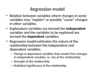
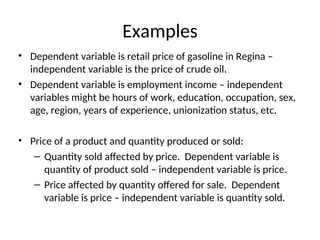
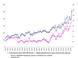
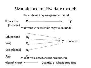
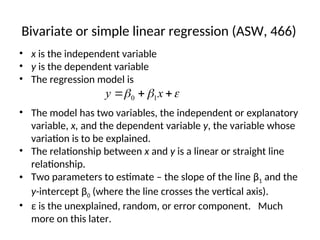
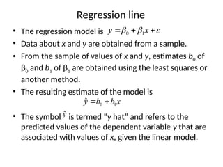
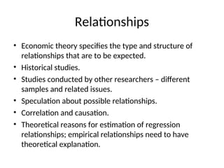
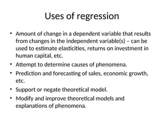
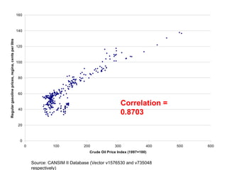
1. Introduction to simple linear
regression
ASW, 12.1-12.2
Economics 224 – Notes for November 5, 2008

2. Regression model
• Relation between variables where changes in some
variables may “explain” or possibly “cause” changes
in other variables.
• Explanatory variables are termed the independent
variables and the variables to be explained are
termed the dependent variables.
• Regression model estimates the nature of the
relationship between the independent and
dependent variables.
– Change in dependent variables that results from changes
in independent variables, ie. size of the relationship.
– Strength of the relationship.
– Statistical significance of the relationship.

3. Examples
• Dependent variable is retail price of gasoline in Regina –
independent variable is the price of crude oil.
• Dependent variable is employment income – independent
variables might be hours of work, education, occupation, sex,
age, region, years of experience, unionization status, etc.
• Price of a product and quantity produced or sold:
– Quantity sold affected by price. Dependent variable is
quantity of product sold – independent variable is price.
– Price affected by quantity offered for sale. Dependent
variable is price – independent variable is quantity sold.

4. 0
100
200
300
400
500
600
1981M01
1982M01
1983M01
1984M01
1985M01
1986M01
1987M01
1988M01
1989M01
1990M01
1991M01
1992M01
1993M01
1994M01
1995M01
1996M01
1997M01
1998M01
1999M01
2000M01
2001M01
2002M01
2003M01
2004M01
2005M01
2006M01
2007M01
2008M01
0
20
40
60
80
100
120
140
160
Crude Oil price index, 1997=100, left axis Regular gasoline prices, regina, cents per litre, right axis
Source: CANSIM II Database (Vector v1576530 and v735048
respectively)

5. Bivariate and multivariate models
(Education) x y
(Income)
(Education) x1
(Sex) x2
(Experience) x3
(Age) x4
y (Income)
Bivariate or simple regression model
Multivariate or multiple regression model
Price of wheat Quantity of wheat produced
Model with simultaneous relationship

6. Bivariate or simple linear regression (ASW, 466)
• x is the independent variable
• y is the dependent variable
• The regression model is
• The model has two variables, the independent or explanatory
variable, x, and the dependent variable y, the variable whose
variation is to be explained.
• The relationship between x and y is a linear or straight line
relationship.
• Two parameters to estimate – the slope of the line β1 and the
y-intercept β0 (where the line crosses the vertical axis).
• ε is the unexplained, random, or error component. Much
more on this later.


 

 x
y 1
0

7. Regression line
• The regression model is
• Data about x and y are obtained from a sample.
• From the sample of values of x and y, estimates b0 of
β0 and b1 of β1 are obtained using the least squares or
another method.
• The resulting estimate of the model is
• The symbol is termed “y hat” and refers to the
predicted values of the dependent variable y that are
associated with values of x, given the linear model.


 

 x
y 1
0
x
b
b
y 1
0
ˆ 

ŷ

8. Relationships
• Economic theory specifies the type and structure of
relationships that are to be expected.
• Historical studies.
• Studies conducted by other researchers – different
samples and related issues.
• Speculation about possible relationships.
• Correlation and causation.
• Theoretical reasons for estimation of regression
relationships; empirical relationships need to have
theoretical explanation.

9. Uses of regression
• Amount of change in a dependent variable that results
from changes in the independent variable(s) – can be
used to estimate elasticities, returns on investment in
human capital, etc.
• Attempt to determine causes of phenomena.
• Prediction and forecasting of sales, economic growth,
etc.
• Support or negate theoretical model.
• Modify and improve theoretical models and
explanations of phenomena.

10. Income hrs/week Income hrs/week
8000 38 8000 35
6400 50 18000 37.5
2500 15 5400 37
3000 30 15000 35
6000 50 3500 30
5000 38 24000 45
8000 50 1000 4
4000 20 8000 37.5
11000 45 2100 25
25000 50 8000 46
4000 20 4000 30
8800 35 1000 200
5000 30 2000 200
7000 43 4800 30

11. Summer Income as a Function of Hours Worked
0
5000
10000
15000
20000
25000
30000
0 10 20 30 40 50 60
Hours per Week
Income

12. x
y 297
2461
ˆ 


R2
= 0.311
Significance = 0.0031

15. 15
Outliers
• Rare, extreme values may distort the
outcome.
– Could be an error.
– Could be a very important observation.
• Outlier: more than 3 standard deviations from
the mean.

16. GPA vs. Time Online
0
2
4
6
8
10
12
50 55 60 65 70 75 80 85 90 95 100
GPA
Time
Online

17. GPA vs. Time Online
0
1
2
3
4
5
6
7
8
9
50 55 60 65 70 75 80 85 90 95 100
GPA
Time
Online

18. 0
20
40
60
80
100
120
140
160
0 100 200 300 400 500 600
Crude Oil Price Index (1997=100)
Regular
gasoline
prices,
regina,
cents
per
litre
Source: CANSIM II Database (Vector v1576530 and v735048
respectively)
Correlation =
0.8703

19. 19
U-Shaped Relationship
0
2
4
6
8
10
12
0 2 4 6 8 10 12
X
Y
Correlation = +0.12.

20. Next Wednesday, November 12
• Least squares method (ASW, 12.2)
• Goodness of fit (ASW, 12.3)
• Assumptions of model (ASW, 12.4)
• Assignment 5 will be available on UR Courses
by late afternoon Friday, November 7.
• No class on Monday, November 10 but I will
be in the office, CL247, from 2:30 – 4:00 p.m.