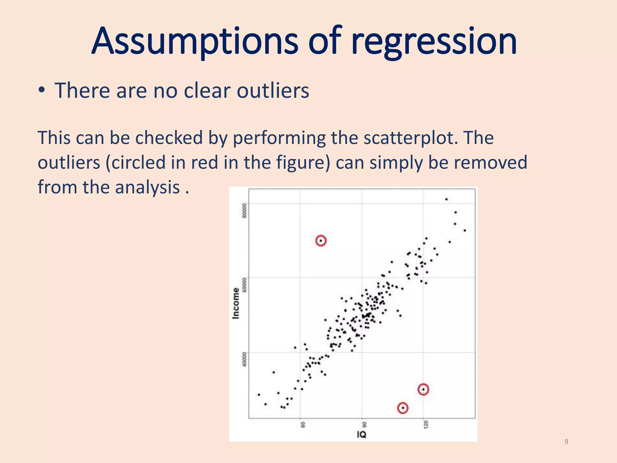
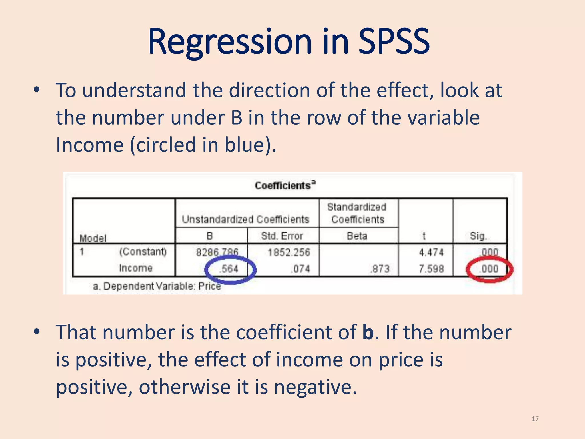
This document provides an introduction to simple linear regression. It explains that regression can be used to study the relationship between two numerical variables, with one as the dependent variable and the other as the independent variable. It discusses the assumptions of regression, including that the relationship is linear and the errors are normally distributed. The document demonstrates how to perform and interpret a simple linear regression in SPSS by investigating the relationship between price of a car and an individual's income. Key outputs to examine are the p-value to determine if the independent variable significantly predicts the dependent variable, and the coefficient to determine the direction of the effect.

1. www.kent.ac.uk/learning
Simple linear regression
1

2. Regression
Introduction
• We will introduce simple linear regression, in particular we will:
• Learn when we can use simple linear regression
• Learn the basic quantities involved in simple linear regression
• Learn how to use regression in real applications
• This presentation is intended for students in initial stages of
Statistics. No previous knowledge is required.
2

3. Regression
• Regression is used to study the relationship
between two variables.
• We can use simple regression if both the
dependent variable (DV) and the independent
variable (IV) are numerical.
•If the DV is numerical but the IV is categorical, it is
best to use ANOVA.
3

4. Examples
The following are situations where we can use
regression:
• Testing if IQ affects income (IQ is the IV and income
is the DV).
• Testing if hours of work affects hours of sleep (DV is
hours of sleep and the hours of work is the IV).
•Testing if the number of cigarettes smoked affects
blood pressure (number of cigarettes smoked is the
IV and blood pressure is the DV).
4

5. Displaying the data
When both the DV and IV are numerical, we can
represent data in the form of a scatterplot.
5

6. Displaying the data
It is important to perform a scatterplot because it
helps us to see if the relationship is linear.
In this example, the
relationship between
body fat % and chance
of heart failure is not
linear and hence it is
not sensible to use
linear regression.

7. Linear model
In regression, the relationship between Y and X is modelled in
the following form:
Y = a + b * X + E
where:
• Y is the dependent variable (Income in the example)
• X is the independent variable (IQ in the example)
• a is an intercept
• b is the coefficient
• E is an error term for each observation (since there is additional
variation not explained by income)
7

8. Assumptions of regression
• The errors E are normally distributed.
This can be tested by plotting an histogram of the residuals
of the regression and checking that they all have a bell shape.
Alternatively, you could use the Shapiro-Wilk test for
normality.
8

9. Assumptions of regression
• There are no clear outliers
This can be checked by performing the scatterplot. The
outliers (circled in red in the figure) can simply be removed
from the analysis .
9

10. Linear model
We are not interested in the intercept a but only in the coefficient
b.
The coefficient b represents the relationship between X and Y.
• If b is positive, X has a positive effect on Y (as X increases, Y increases);
• If b is negative, X has a negative effect on Y (as X increases, Y decreases).
If b = 0, there is no effect of X on Y.
10

11. Hypothesis testing
Regression tests the null hypothesis:
H0 : There is no effect of X on Y, that is, b = 0.
versus the alternative hypothesis:
H1 : There is an effect of X on Y, that is, b is not 0.
If the null hypothesis is rejected, we reject the hypothesis that there is no
relationship and hence we conclude that there is a significant relationship
between X and Y.
11

12. Hypothesis testing
How do we know if rejecting the null hypothesis?
We perform regression in SPSS and look at the p-value
of the coefficient b.
If the p-value is less than 0.05, we reject the null
hypothesis (the variable is significant), otherwise, we do
not reject the null hypothesis (the variable is not
significant).
12

13. Regression in SPSS
(from statistics.leard.com)
13
Assume that you are trying to investigate the
relationship between an individual’s income and the
price they pay for a car.
In the data, assume that the price is encoded in the
variable Price and the income in the variable Income.

14. Regression in SPSS
14
• First, go on Analyze > Regression > Linear..

15. Regression in SPSS
15
• In the Linear Regression box, transfer the DV
(price) to the Dependent box and the IV (income)
to the Independent(s): box
• Finally, click on
the OK Button

16. Regression in SPSS
16
• Look for the box “Coefficients” and identify the
number under Sig. in the row of the variable
Income (circled in red).
• That number is the p-value. If this number (in this
case 0.000) is less than 0.05, the variable Income
is significant, otherwise it is not.

17. Regression in SPSS
17
• To understand the direction of the effect, look at
the number under B in the row of the variable
Income (circled in blue).
• That number is the coefficient of b. If the number
is positive, the effect of income on price is
positive, otherwise it is negative.

18. www.kent.ac.uk/learning
To book a maths/stats appointment…
18

19. Questions?
19