The document discusses various searching, sorting, and hashing techniques used in data structures and algorithms. It describes linear and binary search methods for finding elements in a list or array. It also explains bubble, insertion, selection, and shell sort algorithms for arranging elements in ascending or descending order. Finally, it covers hashing techniques like hash functions, separate chaining, and open addressing that are used to map keys to values in a hash table.
![191ITC301T DATA STRUCTURES AND ALGORITHMS NOTES - IV
UNIT IV : SEARCHING, SORTING AND HASHING TECHNIQUES 9
Searching- Linear Search - Binary Search. Sorting - Bubble sort –Quick Sort - Insertion sort - Merge
sort. Hashing- Hash Functions – Separate Chaining – Open Addressing – Rehashing – Double
Hashing-Extendible Hashing.
Searching is used to find the location where an element is available. There are two types
of search techniques. They are:
● Linear or sequential search
● Binary search
Sorting allows an efficient arrangement of elements within a given data structure. It is a way
in which the elements are organized systematically for some purpose. For example, a
dictionary in which words is arranged in alphabetical order and telephone director in which
the subscriber names are listed in alphabetical order. There are many sorting techniques out
of which we study the following.
• Bubble sort
• Insertion sort
• Selection sort and
• Shell sort
There are two types of sorting techniques:
1.2. Internal sorting
1.3. External sorting
If all the elements to be sorted are present in the main memory then such sorting is called
internal sorting on the other hand, if some of the elements to be sorted are kept on the
secondary storage, it is called external sorting. Here we study only internal sorting
techniques.
Linear Search:
This is the simplest of all searching techniques. In this technique, an ordered or unordered list
will be searched one by one from the beginning until the desired element is found. If the
desired element is found in the list then the search is successful otherwise unsuccessful.
Suppose there are ‗n’ elements organized sequentially on a List. The number of
comparisons required to retrieve an element from the list, purely depends on where the
element is stored in the list. If it is the first element, one comparison will do; if it is second
element two comparisons are necessary and so on. On an average you need [(n+1)/2]
comparison‘s to search an element. If search is not successful, you would need ‘n’
comparisons.
The time complexity of linear search is O(n).](https://image.slidesharecdn.com/unitiv-datastructures-220703042928-43c0891b/75/UNIT-IV-Data-Structures-pdf-1-2048.jpg)
![191ITC301T DATA STRUCTURES AND ALGORITHMS NOTES - IV
Algorithm:
Let array a[n] stores n elements. Determine whether element ‗x‘ is present or not.
linsrch(a[n], x)
{
index = 0;
flag = 0;
while (index < n) do
{
if (x == a[index])
{
flag = 1; break;
}
index ++;
}
if(flag == 1)
printf(―Data found at %d position―, index);
else
printf(―data not found‖);
}
Example :
Let us illustrate linear search on the following 9 elements:
Index 0 1 2 3 4 5 6 7 8
Elements -15 -6 0 7 9 23 54 82 101
Searching different elements is as follows:
Searching for x = 7 Search successful, data found at 3rd
position.
Searching for x = 82 Search successful, data found at 7th
position.
Searching for x = 42 Search un-successful, data not found.
A non-recursive program for Linear Search:
{ include <stdio.h>
{ include <conio.h>
main()
{
int number[25], n, data, i, flag = 0; clrscr();
printf("n Enter the number of elements: "); scanf("%d", &n);
printf("n Enter the elements:
"); for(i = 0; i < n; i++)
scanf("%d", &number[i]);
printf("n Enter the element to be Searched: "); scanf("%d",
&data);
for( i = 0; i < n; i++){](https://image.slidesharecdn.com/unitiv-datastructures-220703042928-43c0891b/75/UNIT-IV-Data-Structures-pdf-2-2048.jpg)
![191ITC301T DATA STRUCTURES AND ALGORITHMS NOTES - IV
if(number[i] == data)
{
flag = 1;
break;
}
}
if(flag == 1)
printf("n Data found at location: %d", i+1);
else
}
printf("n Data not found "); }
A Recursive program for linear search:
include <stdio.h>
include <conio.h>
void linear_search(int a[], int data, int position, int n)
{
if(position < n)
{
if(a[position] == data)
printf("n Data Found at %d ", position);
else
linear_search(a, data, position + 1, n);
}
void main()
{
printf("n Data not found");
int a[25], i, n, data;
clrscr();
printf("n Enter the number of elements: ");
scanf("%d", &n);
printf("n Enter the elements:
"); for(i = 0; i < n; i++)
{
scanf("%d", &a[i]);
}
printf("n Enter the element to be seached: ");
scanf("%d", &data);
linear_search(a, data, 0, n);
getch();
}
BINARY SEARCH
If we have ‗n‘ records which have been ordered by keys so that x1 < x2 < … < xn . When we
are given a element ‗x‘, binary search is used to find the corresponding element from the list.](https://image.slidesharecdn.com/unitiv-datastructures-220703042928-43c0891b/75/UNIT-IV-Data-Structures-pdf-3-2048.jpg)
![191ITC301T DATA STRUCTURES AND ALGORITHMS NOTES - IV
In case ‗x‘ is present, we have to determine a value ‗j‘ such that a[j] = x (successful search).
If ‗x‘ is not in the list then j is to set to zero (un successful search).
In Binary search we jump into the middle of the file, where we find key a[mid], and compare
‗x‘ with a[mid]. If x = a[mid] then the desired record has been found. If x < a[mid] then ‗x‘
must be in that portion of the file that precedes a[mid]. Similarly, if a[mid] > x, then further
search is only necessary in that part of the file which follows a[mid].
If we use recursive procedure of finding the middle key a[mid] of the un-searched portion of
a file, then every un-successful comparison of ‗x‘ with a[mid] will eliminate roughly half the
un-searched portion from consideration.
Since the array size is roughly halved after each comparison between ‗x‘ and a[mid], and
since an array of length ‗n‘ can be halved only about log2n times before reaching a trivial
length, the worst case complexity of Binary search is about log2n.
Algorithm:
Let array a[n] of elements in increasing order, n ≥ 0, determine whether ‗x‘ is present, and if so,
set j such that x = a[j] else return 0.
binsrch(a[], n, x)
{
low = 1; high = n; while (low < high) do
{
mid = (low + high)/2 if (x < a[mid])
high = mid – 1; else if (x > a[mid])
low = mid + 1; else return mid;
}
return 0;
}
low and high are integer variables such that each time through the loop either ‗x‘ is found or low
is increased by at least one or high is decreased by at least one. Thus we have two sequences of
integers approaching each other and eventually low will become greater than high causing
termination in a finite number of steps if ‗x‘ is not present.
Example 1:
Let us illustrate binary search on the following 12 elements:
Index 1 2 3 4 5 6 7 8 9 10 11 12
Elements 4 7 8 9 16 20 24 38 39 45 54 77
If we are searching for x = 4: (This needs 3 comparisons)
low = 1, high = 12, mid = 13/2 = 6, check 20
low = 1, high = 5, mid = 6/2 = 3, check 8
low = 1, high = 2, mid = 3/2 = 1, check 4, found
If we are searching for x = 7: (This needs 4 comparisons)](https://image.slidesharecdn.com/unitiv-datastructures-220703042928-43c0891b/75/UNIT-IV-Data-Structures-pdf-4-2048.jpg)
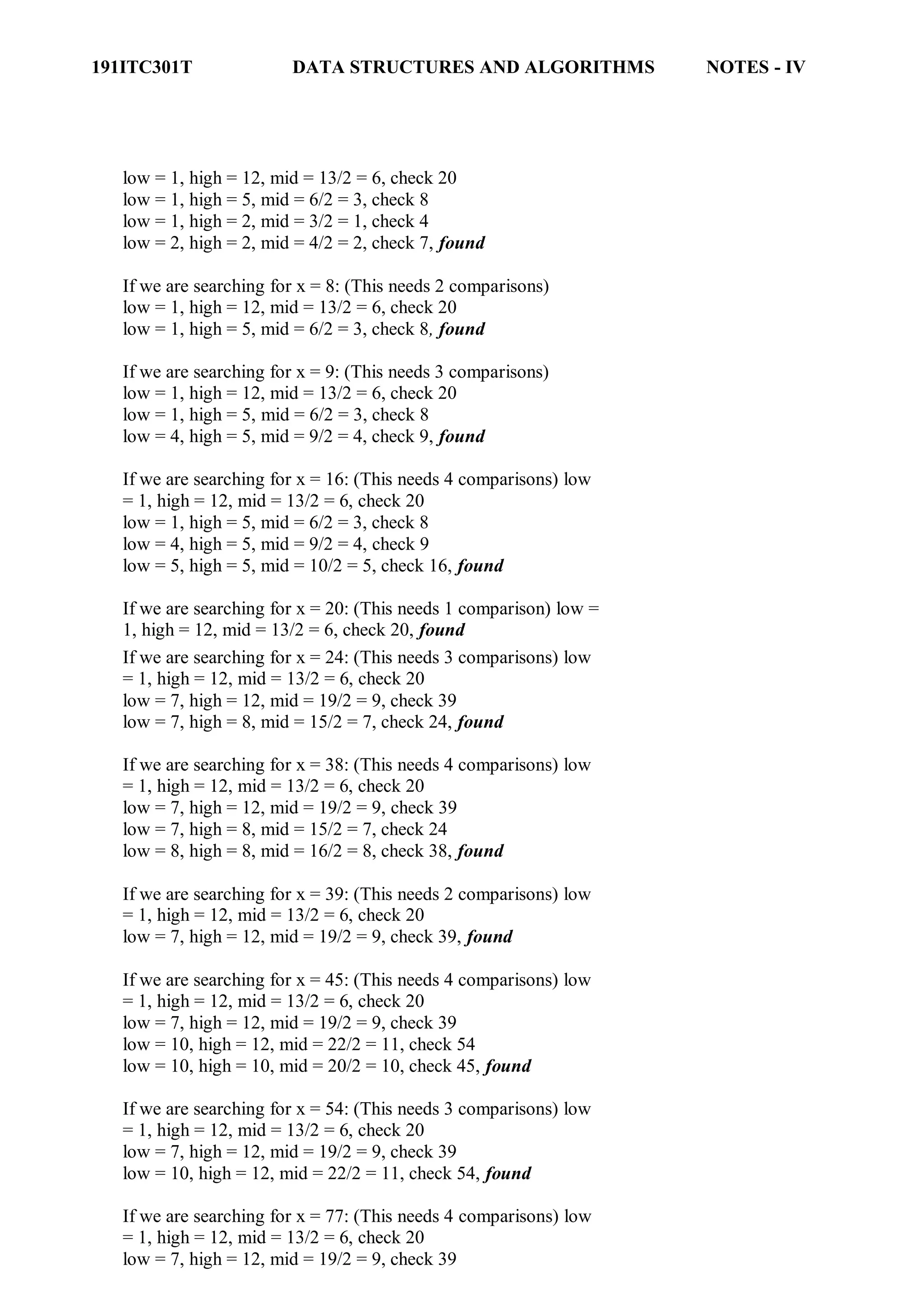
![191ITC301T DATA STRUCTURES AND ALGORITHMS NOTES - IV
low = 10, high = 12, mid = 22/2 = 11, check 54
low = 12, high = 12, mid = 24/2 = 12, check 77, found
The number of comparisons necessary by search element: 20
– requires 1 comparison;
8 and 39 – requires 2 comparisons;
4, 9, 24, 54 – requires 3 comparisons and
7, 16, 38, 45, 77 – requires 4 comparisons
Summing the comparisons, needed to find all twelve items and dividing by 12, yielding
37/12 or approximately 3.08 comparisons per successful search on the average.A non-
recursive program for binary search:
# include <stdio.h> #
include <conio.h>
main()
{
int number[25], n, data, i, flag = 0, low, high, mid; clrscr();
printf("n Enter the number of elements: "); scanf("%d", &n);
printf("n Enter the elements in ascending order: "); for(i = 0; i
< n; i++)
scanf("%d", &number[i]);
printf("n Enter the element to be searched: ");
scanf("%d", &data);
low = 0; high = n-1; while(low
<= high)
{
mid = (low + high)/2;
if(number[mid] == data)
{
}
else
{
flag = 1; break;
if(data < number[mid])
high = mid - 1;
else
}
}
low = mid + 1;
if(flag == 1)
printf("n Data found at location: %d", mid + 1);
else
}
printf("n Data Not Found ");](https://image.slidesharecdn.com/unitiv-datastructures-220703042928-43c0891b/75/UNIT-IV-Data-Structures-pdf-6-2048.jpg)
![191ITC301T DATA STRUCTURES AND ALGORITHMS NOTES - IV
A recursive program for binary search:
# include <stdio.h> #
include <conio.h>
void bin_search(int a[], int data, int low, int high)
{
int mid ;
if( low <= high)
{
mid = (low + high)/2;
if(a[mid] == data)
printf("n Element found at location: %d ", mid + 1);else
{
if(data < a[mid])
bin_search(a, data, low, mid-1);else
bin_search(a, data, mid+1, high);
}
else
printf("n Element not found");
}
void main()
{
int a[25], i, n, data;
clrscr();
printf("n Enter the number of elements: ");
scanf("%d", &n);
printf("n Enter the elements in ascending order: "); for(i
= 0; i < n; i++)
scanf("%d", &a[i]);
printf("n Enter the element to be searched: ");
scanf("%d", &data);
bin_search(a, data, 0, n-1);
getch();
}
Bubble Sort:
The bubble sort is easy to understand and program. The basic idea of bubble sort is to pass
through the file sequentially several times. In each pass, we compare each element in the file
with its successor i.e., X[i] with X[i+1] and interchange two element when they are not in
proper order. We will illustrate this sorting technique by taking a specific example. Bubble
sort is also called as exchange sort.
Example:
Consider the array x[n] which is stored in memory as shown below:](https://image.slidesharecdn.com/unitiv-datastructures-220703042928-43c0891b/75/UNIT-IV-Data-Structures-pdf-7-2048.jpg)
![191ITC301T DATA STRUCTURES AND ALGORITHMS NOTES - IV
X[0] X[1] X[2] X[3] X[4] X[5]
33 44 22 11 66 55
Suppose we want our array to be stored in ascending order. Then we pass through the array
5 times as described below:
Pass 1: (first element is compared with all other elements).
We compare X[i] and X[i+1] for i = 0, 1, 2, 3, and 4, and interchange X[i] and X[i+1] if
X[i] > X[i+1]. The process is shown below:
X[0] X[1] X[2] X[3] X[4] X[5] Remarks
33 44 22 11 66 55
22 44
11 44
44 66
55 66
33 22 11 44 55 66
The biggest number 66 is moved to (bubbled up) the right most position in the array.
Pass 2: (second element is compared).
We repeat the same process, but this time we don‘t include X[5] into our comparisons. i.e.,
we compare X[i] with X[i+1] for i=0, 1, 2, and 3 and interchange X[i] and X[i+1] if X[i] >
X[i+1]. The process is shown below:
X[0] X[1] X[2] X[3] X[4] Remarks
33
22
22
22
33
11
11
11
33
33
33
44
44
44
44
55
55
55
The second biggest number 55 is moved now to X[4].
Pass 3: (third element is compared).
We repeat the same process, but this time we leave both X[4] and X[5]. By doing this, we
move the third biggest number 44 to X[3].](https://image.slidesharecdn.com/unitiv-datastructures-220703042928-43c0891b/75/UNIT-IV-Data-Structures-pdf-8-2048.jpg)
![191ITC301T DATA STRUCTURES AND ALGORITHMS NOTES - IV
X[0] X[1] X[2] X[3] Remarks
22 11 33 44
11 22
22 33
33 44
11 22 33 44
Pass 4: (fourth element is compared).
We repeat the process leaving X[3], X[4], and X[5]. By doing this, we move the fourth
biggest number 33 to X[2].
11 22 33
11 22
22 33
Pass 5: (fifth element is compared).
We repeat the process leaving X[2], X[3], X[4], and X[5]. By doing this, we move the fifth
biggest number 22 to X[1]. At this time, we will have the smallest number 11 in X[0]. Thus,
we see that we can sort the array of size 6 in 5 passes.
For an array of size n, we required (n-1) passes.
Program for Bubble Sort:
#include <stdio.h>
#include <conio.h>
void bubblesort(int x[], int n)
{
int i, j, temp;
for (i = 0; i < n; i++)
{
for (j = 0; j < n–i-1 ; j++)
{
if (x[j] > x[j+1])
{
temp = x[j]; x[j]
= x[j+1]; x[j+1]
= temp;
}
}
}
}
main()](https://image.slidesharecdn.com/unitiv-datastructures-220703042928-43c0891b/75/UNIT-IV-Data-Structures-pdf-9-2048.jpg)
![191ITC301T DATA STRUCTURES AND ALGORITHMS NOTES - IV
{
int i, n, x[25]; clrscr();
printf("n Enter the number of elements: "); scanf("%d", &n);
printf("n Enter Data:");
for(i = 0; i < n ; i++)
scanf("%d", &x[i]);
bubblesort(x, n);
printf ("n Array Elements after sorting: ");
for (i = 0; i < n; i++)
printf ("%5d", x[i]);
}
Selection Sort:
Selection sort will not require no more than n-1 interchanges. Suppose x is an array of size n
stored in memory. The selection sort algorithm first selects the smallest element in the array
x and place it at array position 0; then it selects the next smallest element in the array x and
place it at array position 1. It simply continues this procedure until it places the biggest
element in the last position of the array.
The array is passed through (n-1) times and the smallest element is placed in its respective
position in the array as detailed below:
Pass 1: Find the location j of the smallest element in the array x [0], x[1], x[n-1],
and then interchange x[j] with x[0]. Then x[0] is sorted.
Pass 2: Leave the first element and find the location j of the smallest element in the sub-array
x[1], x[2], . . . . x[n-1], and then interchange x[1] with x[j]. Then x[0], x[1] are sorted.
Pass 3: Leave the first two elements and find the location j of the smallest element in the sub-
array x[2], x[3], . . . . x[n-1], and then interchange x[2] with x[j]. Then x[0], x[1],
x[2] are sorted.
Pass (n-1): Find the location j of the smaller of the elements x[n-2] and x[n-1], and then
interchange x[j] and x[n-2]. Then x[0], x[1], . . . . x[n-2] are sorted. Of course, during
this pass x[n-1] will be the biggest element and so the entire array is sorted.
Example:
Let us consider the following example with 9 elements to analyze selection Sort:
1 2 3 4 5 6 7 8 9 Remarks
65 70 75 80 50 60 55 85 45 find the first smallest element
i j swap a[i] & a[j]
45 70 75 80 50 60 55 85 65 find the second smallest element
i j swap a[i] and a[j]
45 50 75 80 70 60 55 85 65 Find the third smallest element
i j swap a[i] and a[j]](https://image.slidesharecdn.com/unitiv-datastructures-220703042928-43c0891b/75/UNIT-IV-Data-Structures-pdf-10-2048.jpg)
![191ITC301T DATA STRUCTURES AND ALGORITHMS NOTES - IV
45 50 55 80 70 60 75 85 65 Find the fourth smallest element
i j swap a[i] and a[j]
45 50 55 60 70 80 75 85 65 Find the fifth smallest element
i j swap a[i] and a[j]
45 50 55 60 65 80 75 85 70 Find the sixth smallest element
i j swap a[i] and a[j]
45 50 55 60 65 70 75 85 80 Find the seventh smallest
element
i j swap a[i] and a[j]
45 50 55 60 65 70 75 85 80 Find the eighth smallest element
i J swap a[i] and a[j]
45 50 55 60 65 70 75 80 85 The outer loop ends.
Non-recursive Program for selection sort:
# include<stdio.h> #
include<conio.h>
void selectionSort( int low, int high );
int a[25];
int main()
{
int num, i= 0;
clrscr();
printf( "Enter the number of elements: " );
scanf("%d", &num);
printf( "nEnter the elements:n" );
for(i=0; i < num; i++)
scanf( "%d", &a[i] );
selectionSort( 0, num - 1 );
printf( "nThe elements after sorting are: " ); for(
i=0; i< num; i++ )
printf( "%d ", a[i] );
return 0;
}
void selectionSort( int low, int high )
{
int i=0, j=0, temp=0, minindex;
for( i=low; i <= high; i++ )
{
minindex = i;
for( j=i+1; j <= high; j++ )](https://image.slidesharecdn.com/unitiv-datastructures-220703042928-43c0891b/75/UNIT-IV-Data-Structures-pdf-11-2048.jpg)
![191ITC301T DATA STRUCTURES AND ALGORITHMS NOTES - IV
{
if( a[j] < a[minindex] )
minindex = j;
}
temp = a[i];
a[i] = a[minindex];
a[minindex] = temp;
}
}
Insertion sort algorithm
Insertion sort algorithm picks elements one by one and places it to the right position where it
belongs in the sorted list of elements. In the following C program we have implemented the same
logic.
Before going through the program, lets see the steps of insertion sort with the help of an example.
Input elements: 89 17 8 12 0
Step 1: 89 17 8 12 0 (the bold elements are sorted list and non-bold unsorted list)
Step 2: 17 89 8 12 0 (each element will be removed from unsorted list and placed at the right
position in the sorted list)
Step 3: 8 17 89 12 0
Step 4: 8 12 17 89 0
Step 5: 0 8 12 17 89
Algorithm
SELECTION SORT(ARR, N)
o Step 1: Repeat Steps 2 and 3 for K = 1 to N-1
o Step 2: CALL SMALLEST(ARR, K, N, POS)
o Step 3: SWAP A[K] with ARR[POS]
[END OF LOOP]
o Step 4: EXIT
SMALLEST (ARR, K, N, POS)
o Step 1: [INITIALIZE] SET SMALL = ARR[K]
o Step 2: [INITIALIZE] SET POS = K
o Step 3: Repeat for J = K+1 to N -1
IF SMALL > ARR[J]
SET SMALL = ARR[J]
SET POS = J
[END OF IF]
[END OF LOOP]
o Step 4: RETURN POS
Program:](https://image.slidesharecdn.com/unitiv-datastructures-220703042928-43c0891b/75/UNIT-IV-Data-Structures-pdf-12-2048.jpg)
![191ITC301T DATA STRUCTURES AND ALGORITHMS NOTES - IV
#include<stdio.h>
int smallest(int[],int,int);
void main ()
{
int a[10] = {10, 9, 7, 101, 23, 44, 12, 78, 34, 23};
int i,j,k,pos,temp;
for(i=0;i<10;i++)
{
pos = smallest(a,10,i);
temp = a[i];
a[i]=a[pos];
a[pos] = temp;
}
printf("nprinting sorted elements...n");
for(i=0;i<10;i++)
{
printf("%dn",a[i]);
}
}
int smallest(int a[], int n, int i)
{
int small,pos,j;
small = a[i];
pos = i;
for(j=i+1;j<10;j++)
{
if(a[j]<small)
{
small = a[j];
pos=j;
}
}
return pos;
}
Quick Sort
Sorting is a way of arranging items in a systematic manner. Quicksort is the widely used sorting
algorithm that makes n log n comparisons in average case for sorting an array of n elements. It is a
faster and highly efficient sorting algorithm. This algorithm follows the divide and conquer
approach. Divide and conquer is a technique of breaking down the algorithms into subproblems,
then solving the subproblems, and combining the results back together to solve the original problem.
Divide: In Divide, first pick a pivot element. After that, partition or rearrange the array into two
sub-arrays such that each element in the left sub-array is less than or equal to the pivot element and
each element in the right sub-array is larger than the pivot element.
Conquer: Recursively, sort two subarrays with Quicksort.ifference between JDK, JRE, and JVM
Combine: Combine the already sorted array.](https://image.slidesharecdn.com/unitiv-datastructures-220703042928-43c0891b/75/UNIT-IV-Data-Structures-pdf-13-2048.jpg)
![191ITC301T DATA STRUCTURES AND ALGORITHMS NOTES - IV
Quicksort picks an element as pivot, and then it partitions the given array around the picked pivot
element. In quick sort, a large array is divided into two arrays in which one holds values that are
smaller than the specified value (Pivot), and another array holds the values that are greater than the
pivot.
After that, left and right sub-arrays are also partitioned using the same approach. It will continue
until the single element remains in the sub-array.
Choosing the pivot
Picking a good pivot is necessary for the fast implementation of quicksort. However, it is typical to
determine a good pivot. Some of the ways of choosing a pivot are as follows -
Pivot can be random, i.e. select the random pivot from the given array.
Pivot can either be the rightmost element of the leftmost element of the given array.
Select median as the pivot element.
Algorithm
Algorithm:
QUICKSORT (array A, start, end)
{
1 if (start < end)
2 {
3 p = partition(A, start, end)
4 QUICKSORT (A, start, p - 1)
5 QUICKSORT (A, p + 1, end)
6 }
}
Partition Algorithm:
The partition algorithm rearranges the sub-arrays in a place.
PARTITION (array A, start, end)
{
1 pivot ? A[end]
2 i ? start-1
3 for j ? start to end -1 {
4 do if (A[j] < pivot) {](https://image.slidesharecdn.com/unitiv-datastructures-220703042928-43c0891b/75/UNIT-IV-Data-Structures-pdf-14-2048.jpg)
![191ITC301T DATA STRUCTURES AND ALGORITHMS NOTES - IV
5 then i ? i + 1
6 swap A[i] with A[j]
7 }}
8 swap A[i+1] with A[end]
9 return i+1
}
Working of Quick Sort Algorithm
Let the elements of array are -
In the given array, we consider the leftmost element as pivot. So, in this case, a[left] = 24, a[right]
= 27 and a[pivot] = 24.
Since, pivot is at left, so algorithm starts from right and move towards left.
Now, a[pivot] < a[right], so algorithm moves forward one position towards left, i.e. -
Now, a[left] = 24, a[right] = 19, and a[pivot] = 24.](https://image.slidesharecdn.com/unitiv-datastructures-220703042928-43c0891b/75/UNIT-IV-Data-Structures-pdf-15-2048.jpg)
![191ITC301T DATA STRUCTURES AND ALGORITHMS NOTES - IV
Because, a[pivot] > a[right], so, algorithm will swap a[pivot] with a[right], and pivot moves to right,
as -
Now, a[left] = 19, a[right] = 24, and a[pivot] = 24. Since, pivot is at right, so algorithm starts from
left and moves to right.
As a[pivot] > a[left], so algorithm moves one position to right as -
Now, a[left] = 9, a[right] = 24, and a[pivot] = 24. As a[pivot] > a[left], so algorithm moves one
position to right as -
Now, a[left] = 29, a[right] = 24, and a[pivot] = 24. As a[pivot] < a[left], so, swap a[pivot] and
a[left], now pivot is at left, i.e. -](https://image.slidesharecdn.com/unitiv-datastructures-220703042928-43c0891b/75/UNIT-IV-Data-Structures-pdf-16-2048.jpg)
![191ITC301T DATA STRUCTURES AND ALGORITHMS NOTES - IV
Since, pivot is at left, so algorithm starts from right, and move to left. Now, a[left] = 24, a[right] =
29, and a[pivot] = 24. As a[pivot] < a[right], so algorithm moves one position to left, as -
Now, a[pivot] = 24, a[left] = 24, and a[right] = 14. As a[pivot] > a[right], so, swap a[pivot] and
a[right], now pivot is at right, i.e. -
Now, a[pivot] = 24, a[left] = 14, and a[right] = 24. Pivot is at right, so the algorithm starts from left
and move to right.](https://image.slidesharecdn.com/unitiv-datastructures-220703042928-43c0891b/75/UNIT-IV-Data-Structures-pdf-17-2048.jpg)
![191ITC301T DATA STRUCTURES AND ALGORITHMS NOTES - IV
Now, a[pivot] = 24, a[left] = 24, and a[right] = 24. So, pivot, left and right are pointing the same
element. It represents the termination of procedure.
Element 24, which is the pivot element is placed at its exact position.
Elements that are right side of element 24 are greater than it, and the elements that are left side of
element 24 are smaller than it.
Now, in a similar manner, quick sort algorithm is separately applied to the left and right sub-arrays.
After sorting gets done, the array will be -
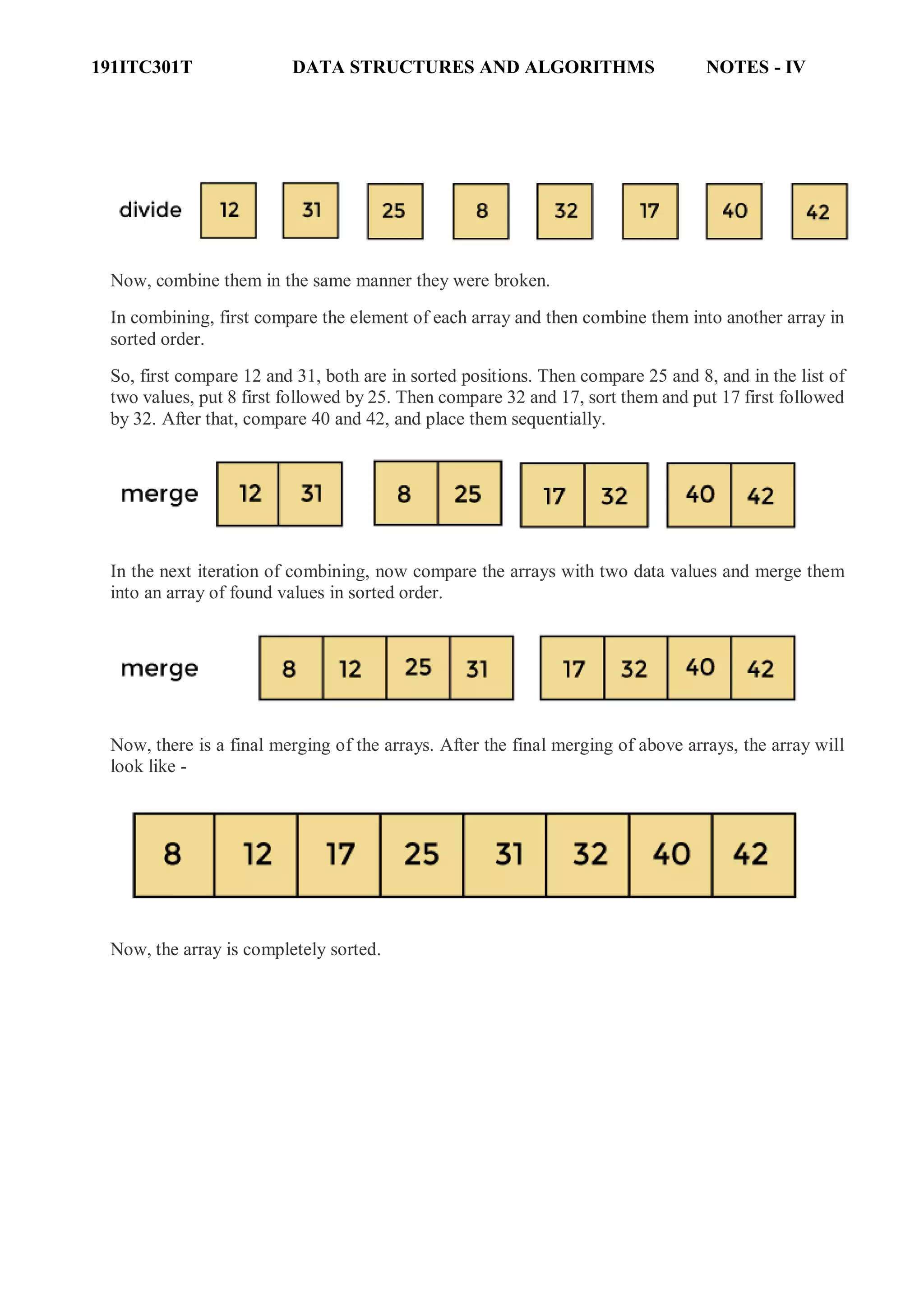
Merge Sort
Merge sort is similar to the quick sort algorithm as it uses the divide and conquer approach to sort
the elements. It is one of the most popular and efficient sorting algorithm. It divides the given list
into two equal halves, calls itself for the two halves and then merges the two sorted halves. We have
to define the merge() function to perform the merging.
The sub-lists are divided again and again into halves until the list cannot be divided further. Then
we combine the pair of one element lists into two-element lists, sorting them in the process. The
sorted two-element pairs is merged into the four-element lists, and so on until we get the sorted list.
Algorithm
In the following algorithm, arr is the given array, beg is the starting element, and end is the last
element of the array.](https://image.slidesharecdn.com/unitiv-datastructures-220703042928-43c0891b/75/UNIT-IV-Data-Structures-pdf-18-2048.jpg)
![191ITC301T DATA STRUCTURES AND ALGORITHMS NOTES - IV
MERGE_SORT(arr, beg, end)
if beg < end
set mid = (beg + end)/2
MERGE_SORT(arr, beg, mid)
MERGE_SORT(arr, mid + 1, end)
MERGE (arr, beg, mid, end)
end of if
END MERGE_SORT
The important part of the merge sort is the MERGE function. This function performs the merging
of two sorted sub-arrays that are A[beg…mid] and A[mid+1…end], to build one sorted
array A[beg…end]. So, the inputs of the MERGE function are A[], beg, mid, and end.
The implementation of the MERGE function is given as follows -
/* Function to merge the subarrays of a[] */
void merge(int a[], int beg, int mid, int end)
{
int i, j, k;
int n1 = mid - beg + 1;
int n2 = end - mid;
int LeftArray[n1], RightArray[n2]; //temporary arrays
/* copy data to temp arrays */
for (int i = 0; i < n1; i++)
LeftArray[i] = a[beg + i];
for (int j = 0; j < n2; j++)
RightArray[j] = a[mid + 1 + j];
i = 0, /* initial index of first sub-array */
j = 0; /* initial index of second sub-array */
k = beg; /* initial index of merged sub-array */
while (i < n1 && j < n2)
{
if(LeftArray[i] <= RightArray[j])
{
a[k] = LeftArray[i];
i++;
}
else
{
a[k] = RightArray[j];
j++;
}
k++;](https://image.slidesharecdn.com/unitiv-datastructures-220703042928-43c0891b/75/UNIT-IV-Data-Structures-pdf-19-2048.jpg)
![191ITC301T DATA STRUCTURES AND ALGORITHMS NOTES - IV
}
while (i<n1)
{
a[k] = LeftArray[i];
i++;
k++;
}
while (j<n2)
{
a[k] = RightArray[j];
j++;
k++;
}
}
Working of Merge sort Algorithm
Now, let's see the working of merge sort Algorithm.
To understand the working of the merge sort algorithm, let's take an unsorted array. It will be easier
to understand the merge sort via an example.
Let the elements of array are -
According to the merge sort, first divide the given array into two equal halves. Merge sort keeps
dividing the list into equal parts until it cannot be further divided.
As there are eight elements in the given array, so it is divided into two arrays of size 4.
Now, again divide these two arrays into halves. As they are of size 4, so divide them into new arrays
of size 2.
Now, again divide these arrays to get the atomic value that cannot be further divided.](https://image.slidesharecdn.com/unitiv-datastructures-220703042928-43c0891b/75/UNIT-IV-Data-Structures-pdf-20-2048.jpg)
![191ITC301T DATA STRUCTURES AND ALGORITHMS NOTES - IV
typedef int INDEX;
A simple hash function
INDEX hash( char *key, int tablesize )
{
int hash_val = 0;
while( *key != '0' )
hash_val += *key++;
return( hash_val % H_SIZE );
}
Another hash function is that, key has at least two characters plus the NULL terminator.
27 represents the number of letters in the English alphabet, plus the blank, and 729 is 272
.
INDEX hash( char *key, int tablesize )
{
return ( ( key[0] + 27*key[1] + 729*key[2] ) % tablesize );
}
A good hash function
INDEX hash( char *key, int tablesize )
{
int hash_val = O;
while( *key != '0' )
hash_val = ( hash_val << 5 ) + *key++;
return( hash_val % H_SIZE );
}
The main problems deal with choosing a function,](https://image.slidesharecdn.com/unitiv-datastructures-220703042928-43c0891b/75/UNIT-IV-Data-Structures-pdf-23-2048.jpg)
![191ITC301T DATA STRUCTURES AND ALGORITHMS NOTES - IV
};
Initialization routine for open hash table
HASHTABLE initializetable(int tablesize )
{
HASHTABLE H;
int i;
if( table size < MIN_TABLE_SIZE )
{
error("Table size too small");
return NULL;
}
H = (HASH_TABLE) malloc ( sizeof (struct hashtbl) );
if( H == NULL )
fatalerror("Out of space!!!");
H->tablesize = nextprime( tablesize );
H->thelists = malloc( sizeof (LIST) * H->tablesize );
if( H->thelists == NULL )
fatalerror("Out of space!!!");
for(i=0; i<H->tablesize; i++ )
{
H->thelists[i] = malloc( sizeof (struct listnode) );
if( H->thelists[i] == NULL )
fatalerror("Out of space!!!");](https://image.slidesharecdn.com/unitiv-datastructures-220703042928-43c0891b/75/UNIT-IV-Data-Structures-pdf-26-2048.jpg)
![191ITC301T DATA STRUCTURES AND ALGORITHMS NOTES - IV
else
H->thelists[i]->next = NULL;
}
return H;
}
Routine for Find operation
Position find( elementtype key, HASHTABLE H )
{
position p;
LIST L;
L = H->thelists[ hash( key, H->tablesize) ];
p = L->next;
while( (p != NULL) && (p->element != key)
) p = p->next;
return p;
}
Routine For Insert Operation
Void insert( elementtype key, HASHTABLE H )
{
position pos, newcell; LIST L;
pos = find( key, H );](https://image.slidesharecdn.com/unitiv-datastructures-220703042928-43c0891b/75/UNIT-IV-Data-Structures-pdf-27-2048.jpg)
![191ITC301T DATA STRUCTURES AND ALGORITHMS NOTES - IV
if( pos == NULL )
{
newcell = (position) malloc(sizeof(struct listnode));
if( newcell == NULL )
fatalerror("Out of space!!!");
else
{
L = H->thelists[ hash( key, H->table size )
]; newcell->next = L->next;
newcell->element =
key; L->next = newcell;
} } }
Closed Hashing (Open Addressing)
Separate chaining has the disadvantage of requiring pointers. This tends to slow the
algorithm down a bit because of the time required to allocate new cells, and also essentially
requires the implementation of a second data structure.
Closed hashing, also known as open addressing, is an alternative to resolving collisions
with linked lists.
In a closed hashing system, if a collision occurs, alternate cells are tried until an empty
cell is found. More formally, cells h0(x), h1(x), h2(x), . . . are tried in succession where hi(x) =
(hash(x) + F(i) mod tablesize), with F(0) = 0. The function, F , is the collision resolution strategy.
Because all the data goes inside the table, a bigger table is needed for closed hashing than for
open hashing. Generally, the load factor should be below = 0.5 for closed hashing.](https://image.slidesharecdn.com/unitiv-datastructures-220703042928-43c0891b/75/UNIT-IV-Data-Structures-pdf-28-2048.jpg)
![191ITC301T DATA STRUCTURES AND ALGORITHMS NOTES - IV
int i;
if( table_size < MIN_TABLE_SIZE )
{
error("Table size too small");
return NULL;
}
H = (hashtable) malloc( sizeof ( struct hash_tbl ) );
if( H == NULL )
fatal_error("Out of space!!!");
H->table_size = next_prime( table_size );
H->the cells = (cell *) malloc ( sizeof ( cell ) * H->table_size );
if( H->the_cells == NULL )
fatal_error("Out of space!!!");
for(i=0; i<H->table_size; i++
) H->the_cells[i].info =
empty; return H;
}
Find routine for closed hashing with quadratic probing
Position find( element_type key, hashtable H )
{
position i, current_pos;
i = 0;
current_pos = hash( key, H->table_size );](https://image.slidesharecdn.com/unitiv-datastructures-220703042928-43c0891b/75/UNIT-IV-Data-Structures-pdf-32-2048.jpg)
![191ITC301T DATA STRUCTURES AND ALGORITHMS NOTES - IV
while( (H->the_cells[current_pos].element != key ) && (H-> the_cells[current_pos]
.info != empty ) )
{
current_pos += 2*(++i) - 1;
if( current_pos >= H->table_size )
current_pos -= H->table_size;
}
return current_pos;
}
Insert routine for closed hash tables with quadratic probing
Void insert( element_type key, hashtable H )
{
position pos;
pos = find( key, H );
if( H->the_cells[pos].info != legitimate )
{ /* ok to insert here */
H->the_cells[pos].info = legitimate;
H->the_cells[pos].element = key;
}
}
Double Hashing
The last collision resolution method we will examine is double hashing. For double hashing, one
popular choice is f(i) = i h2 (x). This formula says that we apply a second hash function to x and
probe at a distance h2 (x), 2 h2 (x), . . ., and so on. A function such as h2 (x) = R - (x mod R),](https://image.slidesharecdn.com/unitiv-datastructures-220703042928-43c0891b/75/UNIT-IV-Data-Structures-pdf-33-2048.jpg)
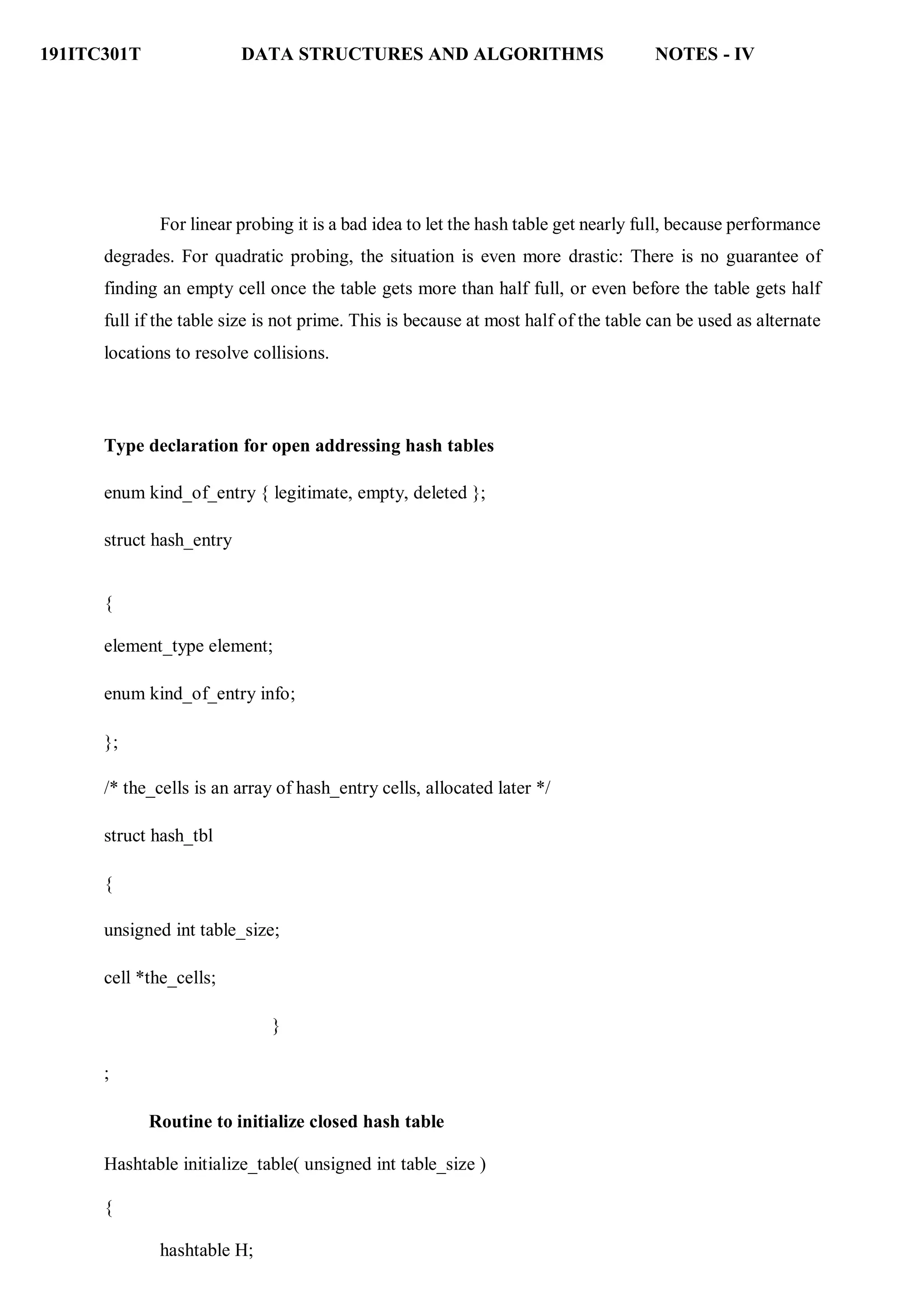
![191ITC301T DATA STRUCTURES AND ALGORITHMS NOTES - IV
This entire operation is called rehashing. This is obviously a very expensive operation – the running time
is O(n).
Rehashing routines
Hashtable rehash( HASH_TABLE H )
{
unsigned int i, old_size;
cell *old_cells;
old_cells = H->the_cells;
old_size = H->table_size;
/* Get a new, empty table */
H = initialize_table( 2*old_size );
/* Scan through old table, reinserting into new */
for( i=0; i<old_size; i++ )
if( old_cells[i].info == legitimate )
insert( old_cells[i].element, H );
free( old_cells );
return H;
}
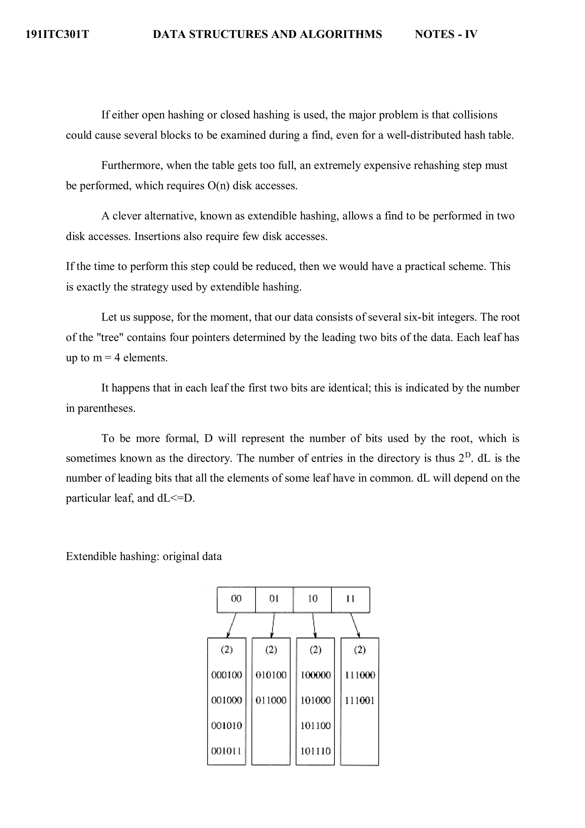
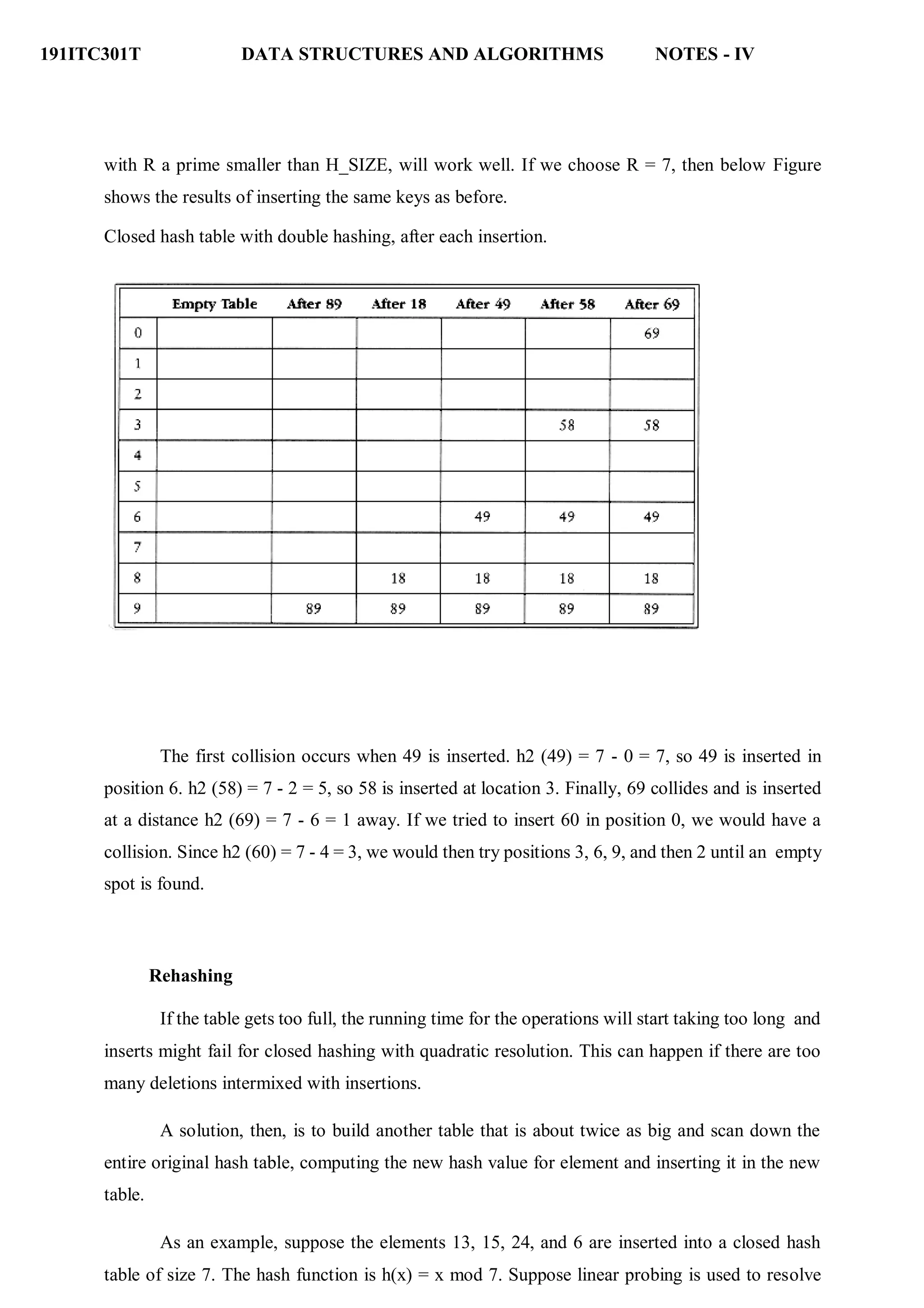
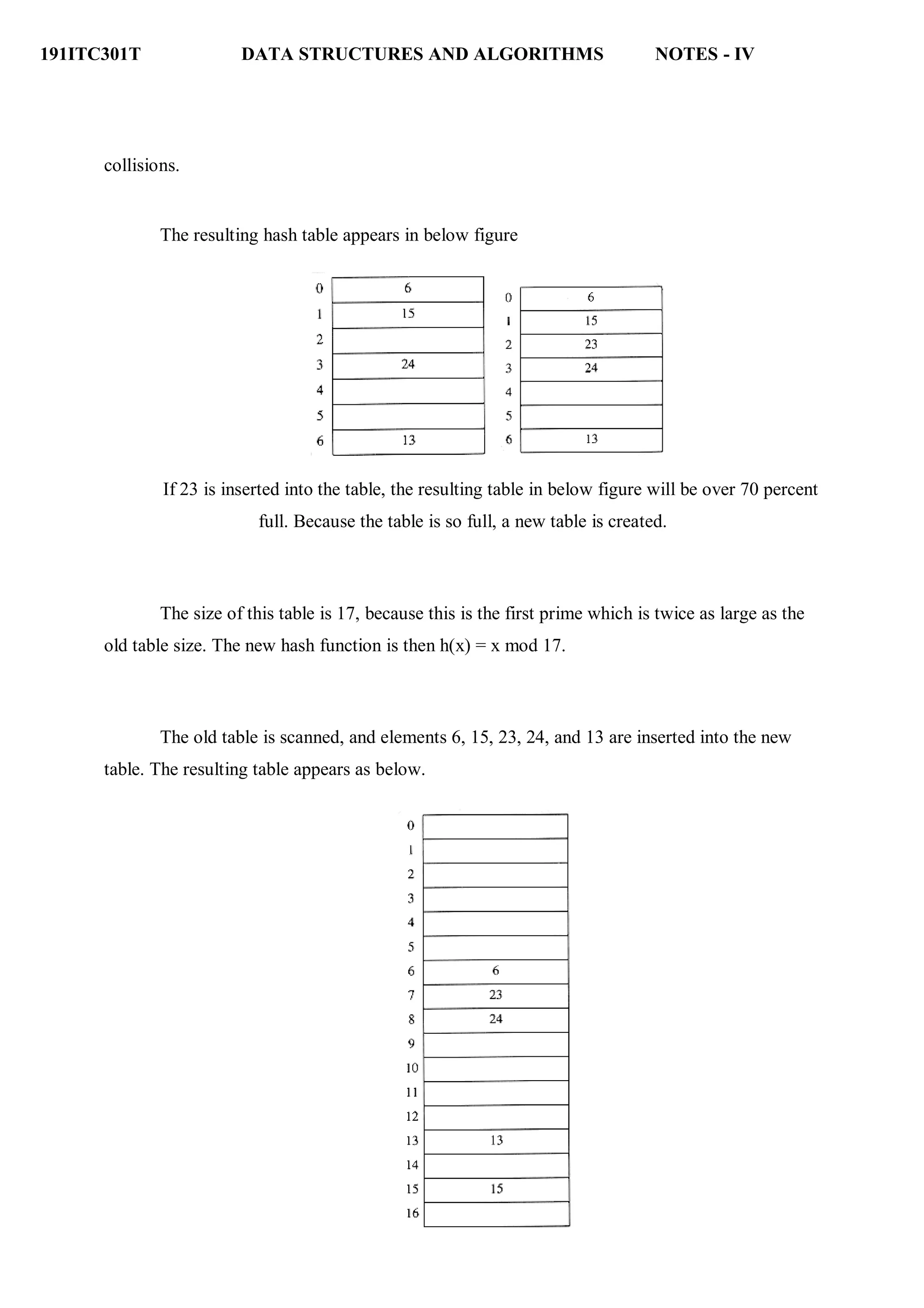
Extendible Hashing
If the amount of data is too large to fit in main memory, then is the number of disk accesses
required to retrieve data. As before, we assume that at any point we have n records to store; the
value of n changes over time. Furthermore, at most m records fit in one disk block. We will use
m = 4 in this section.](https://image.slidesharecdn.com/unitiv-datastructures-220703042928-43c0891b/75/UNIT-IV-Data-Structures-pdf-36-2048.jpg)