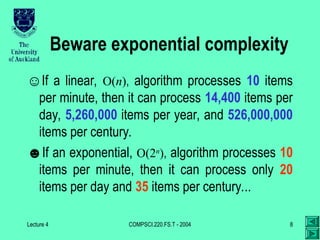
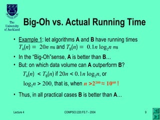
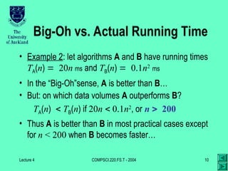
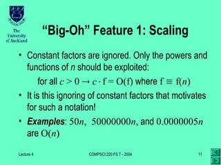
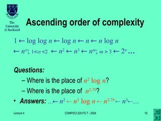
Lecture 4 COMPSCI.220.FS.T - 2004 1
Time Complexity of Algorithms
• If running time T(n) is O(f(n)) then the function
f measures time complexity
– Polynomial algorithms: T(n) is O(nk
); k = const
– Exponential algorithm: otherwise
• Intractable problem: if no polynomial algorithm
is known for its solution
Lecture 4 COMPSCI.220.FS.T - 2004 2
Answer these questions
Running time T(n) Complexity O(n)
n2
+ 100 n + 1
0.001n3
+ n2
+ 1
23 n
23n
23+n
23n
Lecture 4 COMPSCI.220.FS.T - 2004 3
Answer these questions
Running time T(n) Complexity O(n)
0.0001 n + 10000
100000 n + 10000
0.0001 n2
+ 10000 n
100000 n2
+ 10000 n
30 log20(23n)
actually NOT that hard…
Lecture 4 COMPSCI.220.FS.T - 2004 4
Big-Omega
• The function g(n) is (f(n)) iff there exist a real
positive constant c > 0 and a positive integer n0
such that g(n)  cf(n) for all n  n0
– Big Omega is just opposite to Big Oh
– It generalises the concept of “lower bound” () in the
same way as Big Oh generalises the concept of
“upper bound” (≤)
– If f(n) is (g(n)) then g(n) is (f(n))
Lecture 4 COMPSCI.220.FS.T - 2004 5
Big-Theta
• The function g(n) is (f(n)) iff there exist two
real positive constants c1 > 0 and c2 > 0 and a
positive integer n0 such that:
c1f(n)  g(n)  c2f(n) for all n  n0
– Whenever two functions, f and g, are of the same
order, g(n) is (f(n)), they are each Big-Oh of the
other: g(n) is (f(n)) AND f(n) is (g(n))
Lecture 4 COMPSCI.220.FS.T - 2004 6
Upper bounds of complexity
“Big-Oh” specifies an upper bound of complexity so
that the following (and like) relationships hold:
1  O(log n)  O(n) O(n log n)  …
log n  O(n)  O(n log n)  O(n);  …
n  O(n log n)  O(n);  > 1  O(2n
) …
n log n  O(n);  > 1 O(nk
); k   …
nk
 O(n);  > k = O(2n
) = …
Lecture 4 COMPSCI.220.FS.T - 2004 7
Time complexity growth
f(n) Number of data items processed per:
1 minute 1 day 1 year 1 century
n 10 14,400 5.26106
5.26108
n log n 10 3,997 883,895 6.72107
n1.5
10 1,275 65,128 1.40106
n2
10 379 7,252 72,522
n3
10 112 807 3,746
2n
10 20 29 35
Lecture 4 COMPSCI.220.FS.T - 2004 8
Beware exponential complexity
☺If a linear, O(n), algorithm processes 10 items
per minute, then it can process 14,400 items per
day, 5,260,000 items per year, and 526,000,000
items per century.
☻If an exponential, O(2n
), algorithm processes 10
items per minute, then it can process only 20
items per day and 35 items per century...
Lecture 4 COMPSCI.220.FS.T - 2004 9
Big-Oh vs. Actual Running Time
• Example 1: let algorithms A and B have running times
TA(n) 20n ms and TB(n) 0.1n log2n ms
• In the “Big-Oh”sense, A is better than B…
• But: on which data volume can A outperform B?
TA(n) TB(n) if 20n  0.1n log2n, or
log2n  200, that is, when n 2200
≈ 1060
!
• Thus, in all practical cases B is better than A…
Lecture 4 COMPSCI.220.FS.T - 2004 10
Big-Oh vs. Actual Running Time
• Example 2: let algorithms A and B have running times
TA(n) 20n ms and TB(n) 0.1n2
ms
• In the “Big-Oh”sense, A is better than B…
• But: on which data volumes A outperforms B?
TA(n) TB(n) if 20n  0.1n2
, or n 200
• Thus A is better than B in most practical cases except
for n < 200 when B becomes faster…
Lecture 4 COMPSCI.220.FS.T - 2004 11
“Big-Oh” Feature 1: Scaling
• Constant factors are ignored. Only the powers and
functions of n should be exploited:
for all c > 0  cf = O(f) where f  f(n)
• It is this ignoring of constant factors that motivates
for such a notation!
• Examples: 50n, 50000000n, and 0.0000005n
are O(n)
Lecture 4 COMPSCI.220.FS.T - 2004 12
“Big-Oh” Feature 2: Transitivity
• If h does not grow faster than g and g does not
grow faster than f, then h does not grow faster
than f:
h = O(g) AND g = O(f)  h = O(f)
• In other words, if f grows faster than g and g
grows faster than h, then f grows faster than h
• Example: h = O(g); g = O(n2
)  h = O(n2
)
Lecture 4 COMPSCI.220.FS.T - 2004 13
Feature 3: The Rule of Sums
• The sum grows as its fastest term:
g1 = O(f1) AND g2 = O(f2)  g1+g2 = O(max{f1,f2})
– if g = O(f) and h = O(f), then g + h = O (f)
– if g = O(f), then g + f = O (f)
• Examples:
– if h = O(n) AND g = O(n2
), then g + h = O(n2
)
– if h = O(n log n) AND g = O(n log log n), then
g + h = O(n log n)
Lecture 4 COMPSCI.220.FS.T - 2004 14
The Rule of Sums
Lecture 4 COMPSCI.220.FS.T - 2004 15
Feature 4: The Rule of Products
• The upper bound for the product of functions is
given by the product of the upper bounds for the
functions:
g1 = O(f1) AND g2 = O(f2)  g1  g2 = O( f1  f2 )
– if g = O(f) and h = O(f), then g  h = O (f2
)
– if g = O(f), then g  h = O (f  h)
• Example:
if h = O(n) AND g = O(n2
), then g  h = O(n3
)
Lecture 4 COMPSCI.220.FS.T - 2004 16
Ascending order of complexity
1  log log n  log n  n  n log n
 n; 1 2  n2
 n3
 nm
; m  3  2n
…
Questions:
– Where is the place of n2
log n?
– Where is the place of n2.79
?
• Answers: … n2
 n2
log n  n2.79
 n3
…

time complexity of algorithm presentation

  • 1.
    Lecture 4 COMPSCI.220.FS.T- 2004 1 Time Complexity of Algorithms • If running time T(n) is O(f(n)) then the function f measures time complexity – Polynomial algorithms: T(n) is O(nk ); k = const – Exponential algorithm: otherwise • Intractable problem: if no polynomial algorithm is known for its solution
  • 2.
    Lecture 4 COMPSCI.220.FS.T- 2004 2 Answer these questions Running time T(n) Complexity O(n) n2 + 100 n + 1 0.001n3 + n2 + 1 23 n 23n 23+n 23n
  • 3.
    Lecture 4 COMPSCI.220.FS.T- 2004 3 Answer these questions Running time T(n) Complexity O(n) 0.0001 n + 10000 100000 n + 10000 0.0001 n2 + 10000 n 100000 n2 + 10000 n 30 log20(23n) actually NOT that hard…
  • 4.
    Lecture 4 COMPSCI.220.FS.T- 2004 4 Big-Omega • The function g(n) is (f(n)) iff there exist a real positive constant c > 0 and a positive integer n0 such that g(n)  cf(n) for all n  n0 – Big Omega is just opposite to Big Oh – It generalises the concept of “lower bound” () in the same way as Big Oh generalises the concept of “upper bound” (≤) – If f(n) is (g(n)) then g(n) is (f(n))
  • 5.
    Lecture 4 COMPSCI.220.FS.T- 2004 5 Big-Theta • The function g(n) is (f(n)) iff there exist two real positive constants c1 > 0 and c2 > 0 and a positive integer n0 such that: c1f(n)  g(n)  c2f(n) for all n  n0 – Whenever two functions, f and g, are of the same order, g(n) is (f(n)), they are each Big-Oh of the other: g(n) is (f(n)) AND f(n) is (g(n))
  • 6.
    Lecture 4 COMPSCI.220.FS.T- 2004 6 Upper bounds of complexity “Big-Oh” specifies an upper bound of complexity so that the following (and like) relationships hold: 1  O(log n)  O(n) O(n log n)  … log n  O(n)  O(n log n)  O(n);  … n  O(n log n)  O(n);  > 1  O(2n ) … n log n  O(n);  > 1 O(nk ); k   … nk  O(n);  > k = O(2n ) = …
  • 7.
    Lecture 4 COMPSCI.220.FS.T- 2004 7 Time complexity growth f(n) Number of data items processed per: 1 minute 1 day 1 year 1 century n 10 14,400 5.26106 5.26108 n log n 10 3,997 883,895 6.72107 n1.5 10 1,275 65,128 1.40106 n2 10 379 7,252 72,522 n3 10 112 807 3,746 2n 10 20 29 35
  • 8.
    Lecture 4 COMPSCI.220.FS.T- 2004 8 Beware exponential complexity ☺If a linear, O(n), algorithm processes 10 items per minute, then it can process 14,400 items per day, 5,260,000 items per year, and 526,000,000 items per century. ☻If an exponential, O(2n ), algorithm processes 10 items per minute, then it can process only 20 items per day and 35 items per century...
  • 9.
    Lecture 4 COMPSCI.220.FS.T- 2004 9 Big-Oh vs. Actual Running Time • Example 1: let algorithms A and B have running times TA(n) 20n ms and TB(n) 0.1n log2n ms • In the “Big-Oh”sense, A is better than B… • But: on which data volume can A outperform B? TA(n) TB(n) if 20n  0.1n log2n, or log2n  200, that is, when n 2200 ≈ 1060 ! • Thus, in all practical cases B is better than A…
  • 10.
    Lecture 4 COMPSCI.220.FS.T- 2004 10 Big-Oh vs. Actual Running Time • Example 2: let algorithms A and B have running times TA(n) 20n ms and TB(n) 0.1n2 ms • In the “Big-Oh”sense, A is better than B… • But: on which data volumes A outperforms B? TA(n) TB(n) if 20n  0.1n2 , or n 200 • Thus A is better than B in most practical cases except for n < 200 when B becomes faster…
  • 11.
    Lecture 4 COMPSCI.220.FS.T- 2004 11 “Big-Oh” Feature 1: Scaling • Constant factors are ignored. Only the powers and functions of n should be exploited: for all c > 0  cf = O(f) where f  f(n) • It is this ignoring of constant factors that motivates for such a notation! • Examples: 50n, 50000000n, and 0.0000005n are O(n)
  • 12.
    Lecture 4 COMPSCI.220.FS.T- 2004 12 “Big-Oh” Feature 2: Transitivity • If h does not grow faster than g and g does not grow faster than f, then h does not grow faster than f: h = O(g) AND g = O(f)  h = O(f) • In other words, if f grows faster than g and g grows faster than h, then f grows faster than h • Example: h = O(g); g = O(n2 )  h = O(n2 )
  • 13.
    Lecture 4 COMPSCI.220.FS.T- 2004 13 Feature 3: The Rule of Sums • The sum grows as its fastest term: g1 = O(f1) AND g2 = O(f2)  g1+g2 = O(max{f1,f2}) – if g = O(f) and h = O(f), then g + h = O (f) – if g = O(f), then g + f = O (f) • Examples: – if h = O(n) AND g = O(n2 ), then g + h = O(n2 ) – if h = O(n log n) AND g = O(n log log n), then g + h = O(n log n)
  • 14.
    Lecture 4 COMPSCI.220.FS.T- 2004 14 The Rule of Sums
  • 15.
    Lecture 4 COMPSCI.220.FS.T- 2004 15 Feature 4: The Rule of Products • The upper bound for the product of functions is given by the product of the upper bounds for the functions: g1 = O(f1) AND g2 = O(f2)  g1  g2 = O( f1  f2 ) – if g = O(f) and h = O(f), then g  h = O (f2 ) – if g = O(f), then g  h = O (f  h) • Example: if h = O(n) AND g = O(n2 ), then g  h = O(n3 )
  • 16.
    Lecture 4 COMPSCI.220.FS.T- 2004 16 Ascending order of complexity 1  log log n  log n  n  n log n  n; 1 2  n2  n3  nm ; m  3  2n … Questions: – Where is the place of n2 log n? – Where is the place of n2.79 ? • Answers: … n2  n2 log n  n2.79  n3 …