Download to read offline
![Preface
Numerical solutions of electromagnetic field problems constitute an area of
paramount interest in academia, industry, and government. Many numerical
techniques exist based on the solutions of both the differential and integral forms
of Maxwell's equations. It is not recognized very often that for electromagnetic
analysis of both conducting and practical linear piecewise homogeneous isotropic
bodies, integral equations are still one of the most versatile techniques that one can
use in both efficiency and accuracy to solve challenging problems including
analysis of electrically large structures.
In this book, our emphasis is to deal primarily with the solution of time
domain integral equations. Time domain integral equations are generally not as
popular as frequency domain integral equations and there are very good reasons
for it. Frequency domain integral equations arise from the solution of the
unconditionally stable elliptic partial differential equations of boundary-value
problems. The time domain integral equations originate from the solution of the
hyperbolic partial differential equations, which are initial value problems. Hence,
they are conditionally stable. Even though many ways to fix this problem have
been proposed over the years, an unconditionally stable scheme still has been a
dream. However, the use of the Laguerre polynomials in the solution of time
domain integral equations makes it possible to numerically solve time domain
problems without the time variable, as it can be eliminated from the computations
associated with the final equations analytically. Of course, another way to
eliminate the time variable is to take the Fourier transform of the temporal
equations, which gives rise to the classical frequency domain methodology. The
computational problem with a frequency domain methodology is that at each
frequency, the computational complexity scales as 6{Ν*) [C(·) denotes of "the
order of, where N is the number of spatial discretizations]. Time domain methods
are often preferred for solving broadband large complex problems over frequency
domain methods as they do not involve the repeated solution of a large complex
matrix equation. The frequency domain solution requires the solution of a large
matrix equation at every frequency step, whereas in the solution of a time domain
integral equation using an implicit method, one only needs to solve a real large
dense matrix once and then use its inverse in the subsequent computations for each
timestep. So that, a time domain method requires only a vector-matrix product of
large dimension at each time step. Thus, in this case, at each timestep, the
computational complexity is 0{N2
). The use of the orthogonal associated Laguerre
functions for the approximation of the transient responses not only has the
advantage of an implicit transient solution technique as the computation time is
quite small, but also separates the space and the time variables, making it possible
to eliminate the time variable from the final computations analytically. Hence, the
numerical dispersion due to time discretizations does not exist for this
methodology. This methodology has been presented in this book. The
xv](https://image.slidesharecdn.com/timeandfrequencydomainsolutionsofemproblemsusingintegralequationsandahybridmethodologyb-250205130750-568a5ba2/75/Time-and-Frequency-Domain-Solutions-of-EM-Problems-Using-Integral-Equations-and-a-Hybrid-Methodology-B-H-Jung-pdf-15-2048.jpg)
![LIST OF SYMBOLS
Surface without singularity
The nth triangular patch
Area of the nth triangular patch
Light Speed in free space
Wave velocity in a media v
Frequency
Iteration variable, / = l,2,...oo, j = ,2,...oo
Wave number; defined as к = ω^με
Length, e.g. length of an edge or a wire segment
Integer, e.g. the mth and nth edges
Positive or negative components (+ or -)
Magnitude of vector r
Scaling factor for temporal basis function
Time
Transient coefficient for Hertz vector u(r,i), v(r,/)
Expansion coefficient for transient coefficient un{t), vn(t)
Magnetic scalar potential
Electric scalar potential
Associated Laguerre function
Directions for the Spherical Coordinates
Permeability
Permittivity
Angular frequency
Wave impedance
Interior or exterior region (1 or 2 )
Radar Cross Section
(pi) = 3.1415
Linear combination coefficients, [0,1]
Order of M"](https://image.slidesharecdn.com/timeandfrequencydomainsolutionsofemproblemsusingintegralequationsandahybridmethodologyb-250205130750-568a5ba2/75/Time-and-Frequency-Domain-Solutions-of-EM-Problems-Using-Integral-Equations-and-a-Hybrid-Methodology-B-H-Jung-pdf-21-2048.jpg)
![2 MATHEMATICAL BASIS OF A NUMERICAL METHOD
Scalars:
Vectors:
Matrices:
Functions:
Set or Fields:
Spaces:
Functionals:
Operators:
Represented by lower case italicized quantities; a, b,
χ,γ,α,β,
Represented by bold roman letters: a, b, x, y, A, B,
Represented by italicized quantities placed inside
brackets; [a], [b], [A], [B],
Represented by italicized roman letters or bold
corresponding to scalar or vector, respectively; fix),
v(y), f(x), g(z), v(y),
Represented by letters in the capital'Euclid Fraktur
font; 21, 03Л , 9Я, С,
Represented by letters in the capital Euclid Math
Two font, §, 1, R, M, W,
Represented by letters in the Lucida Handwriting
font; F, ft P, p,
Represented by letters in the capital Lucida
Calligraphy font; Л,Ъ,С,£,
1.1 ELEMENT AND SPACES
1.1.1 Elements
An element [1,2] is a definable quantity. Some examples of elements are:
(a) Scalar—a number that can be either real or complex. We normally denote
scalars by italicized lowercase Greek or Roman letters, such as a, fi γ, ...
a, b, с
(b) n-tuple vectors—a group of scalars considered as a linear array. We
denote vectors either by boldface lower case letter, x, y, z ..., or by
uppercase letter, such as X, Y, Z. They can also be represented by
matrices, which are characterized by bracketed letters, such as [x], [y], [z],
... or as [X], [Y],[Z], ... Vectors can be represented either as columns
x = x = (1.1a)
or as rows xT
= [xf=[xux2,---,x„] (1.1b)
where the superscript T denotes transpose of a matrix, which is obtained
by interchanging rows and columns. The numbers X·, X2i · · ·ϊ %n аГС called
the components of a vector.](https://image.slidesharecdn.com/timeandfrequencydomainsolutionsofemproblemsusingintegralequationsandahybridmethodologyb-250205130750-568a5ba2/75/Time-and-Frequency-Domain-Solutions-of-EM-Problems-Using-Integral-Equations-and-a-Hybrid-Methodology-B-H-Jung-pdf-24-2048.jpg)
![ELEMENT AND SPACES 3
(с) Matrix—a group of scalars considered as a rectangular array. We denote
matrices by bracketed letters [А], [В], [С], .... The scalar components of a
matrix [A] are labeled ay and are represented by
u
u "i«
3
22 " ' a
2n
*m u
m2
(1.2)
Column and row matrices generally will be considered as vectors. Other
matrices in this chapter will be represented by capital letters.
(d) Function—a rule whereby to each scalar x, there corresponds another
scalar f(x). A function can also be a vector with an argument, which
may be a scalar or a vector. In either case, a vector function will be
characterized as f(x) or f(x).
This hierarchy of elements can be extended indefinitely. For example, there are
matrices of vectors, matrices of functions, functions of vectors, and so on.
1.1.2 Set
A set [2] is a collection of elements considered as a whole. By a set 6 of elements
a, c, d, e, we mean a collection of well-defined entities. By a G Θ, we mean that a
is an element of the set 6, and b g в implies that b does not belong to Θ. We
usually denote sets by placing { } around the elements, (e.g., Θ = {a,c,d,e,...}or
{«.·})·
1.1.3 Field
A collection of elements of a set of # (scalars) are said to form afield $ [1] if they
possess two binary operations, referred to as the sum and the product, such that the
results of these operations on every two elements of £ lead to elements also in £
and the following axioms are satisfied. If a G # and ß G Ъ , then their sum will
be denoted by а + β and their product by αβ. The properties (α+β)£$ and
αβ £$ are referred to as closure under addition and multiplication, respectively.
So, the axioms are as follows:
1. A binary operation, referred to as addition, is defined for every two
elements of 5 and satisfies
(a) a + β = β + α (commutativity of addition)
(b) а + (β + γ) — (α + β) + γ (associativity of addition)
(c) An element Θ exists in # called additive identity (also called zero) if
α+θ=α.](https://image.slidesharecdn.com/timeandfrequencydomainsolutionsofemproblemsusingintegralequationsandahybridmethodologyb-250205130750-568a5ba2/75/Time-and-Frequency-Domain-Solutions-of-EM-Problems-Using-Integral-Equations-and-a-Hybrid-Methodology-B-H-Jung-pdf-25-2048.jpg)
![4 MATHEMATICAL BASIS OF A NUMERICAL METHOD
(d) For each a e 5 , there is an element —a S # such that
a + (—a) = Θ. The element -a is called the additive inverse of a or
simply the negative of a.
2. A binary operation, referred to as the product, is defined for every two
elements of # and satisfies the following:
(a) aß= ßa (commutativity of multiplication)
(b) α{βγ) = {αβ)γ (associativity of multiplication)
(c) An element e exists called multiplicative identity and is denoted by e
such that as ae = a, e ^ Θ . When we deal with real or complex
numbers, e will be defined as 1.
(d) For each element a ^ Θ in #, an element (a~l
)£$ exists called
the multiplicative inverse of a such that a(a~ ) = e.
3. The binary operation referred to as the product is distributive with respect
to the addition operation so that α(β + γ) = aß + αγ.
Thus, a collection of objects forms a field when the concepts of addition,
multiplication, identity, and inverse elements are defined subject to the previous
axioms. It can be shown that $ contains a unique zero element called the additive
identity and a unique unity element called the multiplicative identity.
The two simplest examples of fields are the field of real numbers, which is
called the real field and is defined by ÎH and the field of complex numbers that is
called the complex field and is denoted by €. In these cases, the binary operations
are ordinary addition and multiplication, and the zero element and the identity
element are, respectively, the numbers 0 and 1. Generally, we will be dealing with
the field of real numbers <
K and complex numbers €. However, it is important to
remember that the previous definition is valid for any general field of scalars. For
example, the set of all rational numbers, real numbers, or complex numbers of the
form,c + yf-ld , where с and dare real numbers, also forms afield. However, the
set of integers does not form a field because the property 2(d) stated earlier is not
satisfied. In addition, any 2 x 2 matrices of the form:
a -b
b а
also form a field under usual matrix addition and multiplication when the numbers
a and b are real, but the existence of singular matrices reveals that not all sets of
2 x 2 matrices form a field.
1.1.4 Space
A space [1,2] is a set for which some mathematical structure is defined. We denote
spaces by the Euclid Math Two font as A, B, C, U, V,.... Some examples of
specific spaces are:](https://image.slidesharecdn.com/timeandfrequencydomainsolutionsofemproblemsusingintegralequationsandahybridmethodologyb-250205130750-568a5ba2/75/Time-and-Frequency-Domain-Solutions-of-EM-Problems-Using-Integral-Equations-and-a-Hybrid-Methodology-B-H-Jung-pdf-26-2048.jpg)
![METRIC SPACE 5
(a) Space of the scalar field, denoted as F = {a, ß,/,...} where the elements
а, Д γ, ... are scalar. This space must also contain the sum, difference,
product, and quotient of any two scalars in the field (division by zero
excluded). In the space of scalar field, the only two fields that we need
are the real field ΪΚ and the complex field <£. When the field is <
H (real
numbers), we call F a linear space over the real field or a real linear
space. When the field is € (complex scalars), we call F a linear space
over the complex field, or a complex linear space.
(b) Space of real vectors of n components, denoted R" ={x,y,z,...} where
each vector is an array of the form of Eq. (1.1a) or (1.1 Z>).
(c) Space of complex vectors ofn components, C" = {x,y,z,...} where each
vector is an array, Eq. (1.1a), or (1.16) with the x as complex scalars.
(d) Space of functions continuous on the interval a<x<b , denoted by
[a,b] = {f,g,h,...} where the elements are functions. We use the
convention that closed intervals a<x<b are denoted by [a,b], open
intervals a<x <b by (a,b), and so on. If the functions are real, then we
call the space real R[a,b], and if they are complex, then we call it
complex C[a,b].
Let us now start with the general concept of a space.
1.2 METRIC SPACE
A nonempty set of elements (or points) X containing u, υ, w is said to be a metric
space [1-3], if to each pair of elements u, υ a real number uf(u,v) is associated,
of two arguments called distance between и and υ satisfying
uF(u, v) > 0 for u, v e X and are distinct
ü/T(u,v) — 0 if and only if и = v
&(u,v) = üF{v,u)
Of (и, w) < QF(u, v) + uf'(y, w) (triangle inequality)
This function &f is called the metric or distance function. Once a distance is
available, one can define the notion of a neighborhood for an element, and that
leads up to the concept of convergence. A sequence of points {uk} converges to и
if and only if the sequence of real numbers {(Ж"(и,ик)} converges to 0. We write
the following:
lim uk=u
k—>oo
or ик —> и and say that {щ} converges to и or that {щ} has the limit u, if for each
£ > 0, there exists an index N exists such that <Ж{и,ик )<ε whenever к > N . A
sequence {uk} is called a Cauchy sequence if for each ε > 0 there exists an N
such that (2fum,u )<ε whenever m,p>N . Therefore, a metric space X is
complete if every Cauchy sequence of points from X converges to a limit in X. As
an example, consider the sequence of rational numbers, и,·,](https://image.slidesharecdn.com/timeandfrequencydomainsolutionsofemproblemsusingintegralequationsandahybridmethodologyb-250205130750-568a5ba2/75/Time-and-Frequency-Domain-Solutions-of-EM-Problems-Using-Integral-Equations-and-a-Hybrid-Methodology-B-H-Jung-pdf-27-2048.jpg)
![6 MATHEMATICAL BASIS OF A NUMERICAL METHOD
1 , 1 1 1
u, = 1; м,= 1 + —; ···; u„ = 1 + — + — + ... +
2
1! " 1! 2! (и-1)!
with the metric defined by ëfiu^u ·) = Ц— U: , it can be shown that [2] the
sequence и, converges to a real number q, which is not a rational number.
Therefore, the space of rational numbers is not complete. However, it can be made
complete by enlarging this space to include irrational numbers.
For example, the real line becomes a metric space of the distance between
two real numbers и and v defined as u — v|, and this space is complete [1].
The set of all complex numbers z, = xt + jyt where j = V—1, is a metric
space under the definition [1]
^>
ζλ,ζ2) = ζλ,ζ2 = ^{χλ-χ2)2
+{yx-y2f 0-3)
and the space is complete.
Consider the set of all real-valued continuous functions u(x) and v(x)
defined on the interval a < x < b with the distance function
uTao(u,v)= max u(x)-v(x) ,j 4)
a<x<b v
' '
So if the Cauchy sequence {un(x)} converges to a function u(x) that is necessarily
continuous, then the space Ща, b] is complete, and this is known as completeness
under the uniform metric.
However, if we consider the set of all real-valued continuous functions
u(x) and v(x) on the bounded interval a < x < b but now with the metric:
Щ {u,v) = ^Jb
au{x)-v{x)2
dx (1.5)
then it has been shown [1] that this formula generates a metric space. However,
this space is not complete, as functions with jump discontinuities can be
approximated in the mean-square sense (that is in metric <Ж2 ) by continuous
functions, like in a Fourier series expansion, which approximates a discontinuous
function in the mean.
Just as in the case of rational numbers, we saw that the metric space was
not complete, but it can be completed by including the irrational numbers. Here we
also employ the same methodology; the space of complex-valued functions on
a<x<b can be completed in the metric (Щ by generating the space ll2a,b] of
real-valued functions square integrable in the Lebesque sense [3, pp. 36-40].](https://image.slidesharecdn.com/timeandfrequencydomainsolutionsofemproblemsusingintegralequationsandahybridmethodologyb-250205130750-568a5ba2/75/Time-and-Frequency-Domain-Solutions-of-EM-Problems-Using-Integral-Equations-and-a-Hybrid-Methodology-B-H-Jung-pdf-28-2048.jpg)
![VECTOR SPACE 7
1.3 VECTOR (LINEAR) SPACE
Any linear space can be called a vector space [1] but we usually use the term
"vector space" to imply that the elements are w-tuple vectors of the form as in Eq.
(1.1a) or (1.16). We use the term function space to imply elements that are
functions. The elements of a linear space also are calledpoints of the space.
To define a vector space V, it is necessary to have a set of objects {u}
(usually referred to as elements, vectors, or points), a field of scalars J, and two
binary operations defined on these scalars and vectors. These operations are called
vector additions and scalar multiplications (i.e., the multiplication of a vector by a
scalar).
In conformity with the mathematical literature, [1], with the terms
"vector" or "point", we mean an element of a vector space. This is not to be
confused with the concept of a vector as a directed line segment, commonly used
in engineering terminology.
Let u and v be vectors of V, and let a belong to a field #; then the sum of
u and v denoted by u Θ v and the product of а О u also must be elements of V.
This is called the closure property [1]. A collection of objects forms a vector space
V over a field 5 if the operations of vector addition and multiplication of a vector
by a scalar taken from $ satisfy the following conditions:
1. For any arbitrary vectors u, v, w elements of the space V and any
arbitrary scalars a, ß belonging to a field $, the following properties need
to be satisfied.
(a) u θ v = v 0 u (commutativity of addition)
(b) (u © v) © w = u © (v © w) (associativity of addition)
(c) There is a null vector 0 in this space such that for any u e V , we
have u Θ 0 = u
(d) To every vector u e V there corresponds an element (-u) e V such
that u © (-u) = 0
2. Let 1 denote the identity element of £, then:
(a) 10 u = u
(b) (aß)Ou = aO(ßOu)
It is important to note that a field must contain an identity element, but a
vector space does not need to have a unity element.
3. (a) (a + /?)Ou = (orOu)©(/?Ou) (distributiveproperty)
(b) а О (u 8 v) = (а О u) Θ (а О v)
Thus, any collection of objects whose elements satisfy these axioms with two
well-defined operations (addition of vectors and multiplication by scalars) forms a
vector space. For the sake of mathematical clarity, here we have used the notation
(+,·) for the operation of a field £ and the notation (Φ,Θ) for the operations of
the vector space. Such a distinction in these operations is essential for the proper
understanding of the concepts. Moreover, the operation of the addition of vector
space generally coincides with the addition operation of the field of scalars. Thus,](https://image.slidesharecdn.com/timeandfrequencydomainsolutionsofemproblemsusingintegralequationsandahybridmethodologyb-250205130750-568a5ba2/75/Time-and-Frequency-Domain-Solutions-of-EM-Problems-Using-Integral-Equations-and-a-Hybrid-Methodology-B-H-Jung-pdf-29-2048.jpg)
![8 MATHEMATICAL BASIS OF A NUMERICAL METHOD
from now on, we will replace the symbol ©by + and will drop О in favor of
juxtaposition to denote scalar multiplication.
As an example, the field € of complex numbers may be considered as a
vector space H over the field of real numbers 9Я. In addition, points of a two-
dimensional real space R2
form a vector space over the field of real numbers 9Я.
Also, the set of all functions that are at least twice differentiable and satisfy the
form of d2
x/dt2
+ dx/dt — ax = 0 for a is a constant and forms a linear vector
space L2
over С All real-valued functions /(/) of the real variable t that are
continuous in the interval [a,b] form a vector space under the ordinary definition
of addition and multiplication by a scalar. The null element of this space is a
function that is identically zero in the same interval. However, the set of all
polynomials of degree « (where и is a positive integer) does not form a vector
space under the familiar definition for addition and multiplication by numbers as
the sum of two polynomials of degree « and is not necessarily a polynomial of
degree «, where n is the exponent of the leading nonzero term. The set of all
polynomials of degree < « forms a vector space.
1.3.1 Dependence and Independence of Vectors
A set of vectors x, y, z, ..., w belonging to a vector space V defined over the field
$ are said to be linearly independent [1] if
a + ßy + /z- h//w = 0; with α,β,/,...,μ£ $ (1.6)
implies α = β = γ = ··· = μ = 0. If a nontrivial relation of the previous type
exists, where the coefficients do not vanish altogether, then the elements are said
to be dependent.
1.3.2 Dimension of a Linear Space
If a vector space contains n linearly independent vectors (« is a finite positive
integer) and if all n + 1 vectors ofthat space are linearly dependent, then the vector
space is said to be of dimension и [1].
Any set of и-linearly independent vectors of V is said to form a basis for
that space, if every vector of V can be expressed as a linear combination of
elements ofthat set. If a basis in a linear space contains и-elements, then the space
is called an и-dimensional space or simply an «-space [1].
1.3.3 Subspaces and Linear Manifolds
A subset of elements of a vector space V is said to form a subspace W of V if W
is a vector space under the same law of addition and scalar multiplication defined
for V, over the same field J [1]. So the null element is the smallest subspace of V,
and in a manner of speaking, V is the largest subspace of itself. Because any](https://image.slidesharecdn.com/timeandfrequencydomainsolutionsofemproblemsusingintegralequationsandahybridmethodologyb-250205130750-568a5ba2/75/Time-and-Frequency-Domain-Solutions-of-EM-Problems-Using-Integral-Equations-and-a-Hybrid-Methodology-B-H-Jung-pdf-30-2048.jpg)
![VECTOR SPACE 9
subspace of a finite dimensional vector space is by itself a vector space, it has
some dimension, and the dimension of the subspace cannot exceed that of the
original space.
If x and y are specified elements of a linear vector space V and if a and ß
are arbitrary numbers of the field #, then the set of elements ax + ßy for all a
and ß in 5 forms a linear subspace. We say that this subspace is generated or
spanned by x and y. Similarly, if {x,y,z,..., w} is a set of vectors V, the
collection of elements of the type ax + ßy + уг H (- μ-w; with
α,β,γ,..., μ G $ forms a linear subspace W. This subspace is called the linear
manifold spanned by {x, y, z,..., w}. The linear manifold spanned by these
vectors is the linear subspace of the smallest dimension that contains them.
Once we are dealing with vectors, we can define it by its magnitude and
the rotation or angle between any two vectors. Associated with these properties,
one can define linear spaces based on these two unique properties of a vector.
1.3.4 Normed Linear Space
A normed linear space [2] (real or complex) in which a real valued function ||u)|
(known as the norm of u) is defined to have the following properties:
(a) ||u|| > 0 ; if u ^ 0 (positivity)
(b) ||u|| = 0 ; if and only if u = 0 (definiteness)
(c) ||«u|| = a x ||u|| (linear scaling)
(d) |u + v|| < ||u| + |v| (triangular inequality)
Here a denotes the absolute value for a. A space with a norm associated with
every element of u in V is called a normed space. It is important to note that a
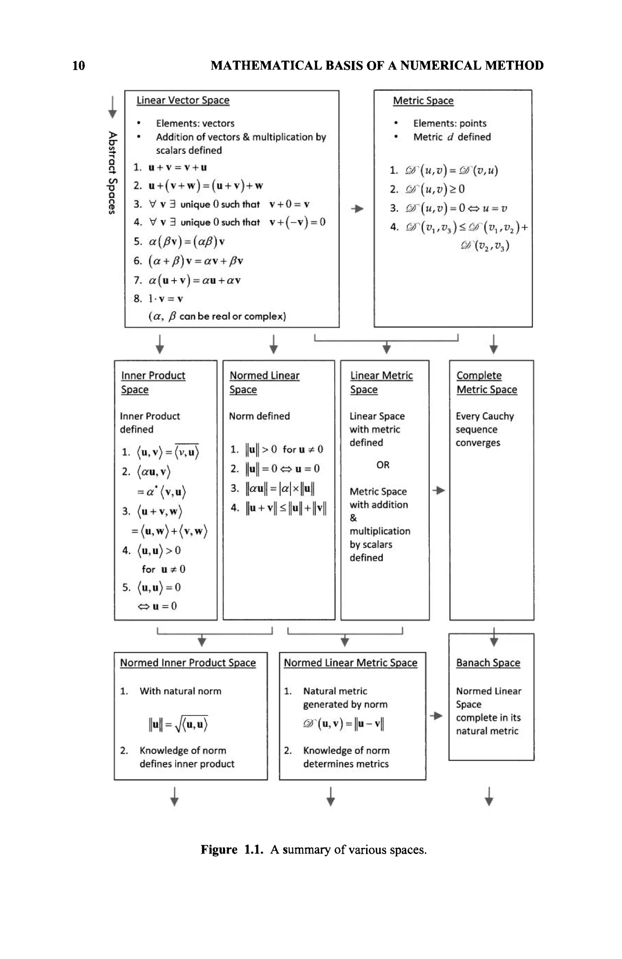
metric space, in general, is different from a normed space. The various hierarchies
of spaces are shown in Figure 1.1.
However, if the metric <Ж(и, v) is identified with the norm so that
<âr(u,v) = |u-v|| (1.7)
then one obtains a normed linear metric space as illustrated in Figure 1.1. So here,
u|| plays the same role as the length of u in an ordinary three-dimensional space.
A normed linear space that is complete in its natural metric, where every Cauchy
sequence converges is called a Banach space, as illustrated in Figure 1.1. The
space of real numbers form a Banach space, but the set of rational numbers does
not constitute a Banach space but a metric space. Similarly, the space of
continuous functions C[a,b] is a Banach space, but the space of square integrable
continuous functions C[a,b] does not form a Banach space.](https://image.slidesharecdn.com/timeandfrequencydomainsolutionsofemproblemsusingintegralequationsandahybridmethodologyb-250205130750-568a5ba2/75/Time-and-Frequency-Domain-Solutions-of-EM-Problems-Using-Integral-Equations-and-a-Hybrid-Methodology-B-H-Jung-pdf-31-2048.jpg)
![VECTOR SPACE 11
Note: Linear spaces may be finite or infinite dimensional.
1.3.5 Inner Product Space
In a normed linear space, a vector has length. We want to refine the structure
further so that the angle between two vectors is also defined. In particular, we want
a criterion for determining whether two vectors are orthogonal, and it is related to
the dotproduct between vectors.
An inner product (u,v) [2] on a complex linear space X<c>
is a
real/complex-valued function of an ordered pair of vectors u, v with the properties
(a) (u,v) = (v,u)
where the overbar denotes the complex conjugate of an expression.](https://image.slidesharecdn.com/timeandfrequencydomainsolutionsofemproblemsusingintegralequationsandahybridmethodologyb-250205130750-568a5ba2/75/Time-and-Frequency-Domain-Solutions-of-EM-Problems-Using-Integral-Equations-and-a-Hybrid-Methodology-B-H-Jung-pdf-33-2048.jpg)
![12 MATHEMATICAL BASIS OF A NUMERICAL METHOD
(b) (au,v) = a(u,v) and (u,ß) = ß (u,v)
where * denotes a complex conjugate of a scalar.
(c) (u + v,w + y) = (u,w) + (v,y) + (v,w) + (u,y)
(d) (u, u) > 0 for u ^ 0 and is a real value,
(u, u) = 0 for u = 0 (the inner product is positive definite)
(e) |(u,v)| <(u,u)(v,v) (equality holds if and only if u and v are
linearly dependent)
Two vectors are orthogonal if their inner product is zero. Orthogonality is
an extension of the geometrical concept of perpendicularity in Ш2
or M3
space.
As an example, in a space with complex elements, the inner product is
given by
(u,v) = n,v*+ u2v*2 + ■■■ + u„v*„ (1.8)
if (u, v) = 0 , then u is geometrically perpendicular to v.
In the space of continuous functions, the inner product is defined in the
complex function space as
(f,g)= fb
f(z)gz)clz (1.9)
О а
So two complex functions are orthogonal if their average is zero; that is,
{i,%) = jj{z)gz)dz = 0 (1.10)
Sometimes it is convenient to define a weighted inner product as follows:
(f,g)= [b
w(z)f(z)gz)dz (1.11)
J a
where w(z) > 0 on [a, b] and is called the weight function. If g is real,
then g(z) will be used instead of g (z).
A space with an inner product associated with any two elements of u and
v in V is called an innerproduct space as shown in Figure 1.1.
One also could obtain a normed inner product space as shown in Figure
1.1 if we identify the norm with the inner product as;
I H ^ T ^ (1.12)
that is, the knowledge of the norm defines the inner product.](https://image.slidesharecdn.com/timeandfrequencydomainsolutionsofemproblemsusingintegralequationsandahybridmethodologyb-250205130750-568a5ba2/75/Time-and-Frequency-Domain-Solutions-of-EM-Problems-Using-Integral-Equations-and-a-Hybrid-Methodology-B-H-Jung-pdf-34-2048.jpg)
![VECTOR SPACE 13
Finally, one could obtain a normed inner product space with its natural
metric as illustrated in Figure 1.1 if we relate the norm, inner product, and the
metric by
^r(u,v) = ||u-v|| = A / ( u - v , u - v ) (1.13)
With the metric defined, we now can use the concept of convergence, which is
repeated here for convenience: A sequence {мк} is said to converge to и if, for
each ε > 0, there exists an N > 0 such that uk - u|| < ε , with k> N .
An inner product space, which is complete in its natural metric, is called a
Hubert space as illustrated in Figure 1.1.
For complex-valued functions u(x) defined in a<x<b, for which the
Lebesque integral
J u(x) dx
a
exists and is finite, we can define
llu
ll2
f u(xfdx (1.14a)
JSÇ(U,V) = | U - V | | 2 = Jjb
u(x)-v(x)2
dx (1.14b)
and the norm is called the JS^ norm. The Cauchy-Schwartz inequality becomes
Г u(x)v*{x)dx < A I u(x)2
dx x Jj v(x) dx (1-15)
The space C[a,b] of continuous functions (real- or complex-valued) on a bounded
interval a<x<b is a normed space under the definition
u = max
1
1 llo
° a<x<b
l"W| (1.16)
This norm generates the natural metric
^ O ( u , v ) = ||u-v|o o = maxu(x)-v(x) ( U 7 )
and C[a,b] can be shown to be a Banach space — a complete normed space [2],
as this norm cannot be derived from an inner product. The reason that this space is](https://image.slidesharecdn.com/timeandfrequencydomainsolutionsofemproblemsusingintegralequationsandahybridmethodologyb-250205130750-568a5ba2/75/Time-and-Frequency-Domain-Solutions-of-EM-Problems-Using-Integral-Equations-and-a-Hybrid-Methodology-B-H-Jung-pdf-35-2048.jpg)
![14 MATHEMATICAL BASIS OF A NUMERICAL METHOD
not a Hubert space but a Banach space is because the inner product cannot be
generated for this metric.
Let Ω be a bounded domain in 9t" with a boundary Γ. Consider the set 6
of real-valued functions that are continuous and have a continuous gradient on Ω.
The following bilinear form
( ρ , 4 > 6 = / η ( ν « . ν ν ) Λ (1.18)
is an admissible inner product on M. The completion of M in the norm generated
by this inner product is known as the Sobolev Space Η'(Ω). This is a subset of a
Hubert space [2]. The term "completion of space M" implies that the limit point of
some sequence of functions is not a member of that space and that these elements
need to be added so as to make the space complete. For example, if we take a
sequence of square integrable functions that are continuous and forms a space
Q, then the limit point of the sequence of continuous functions may result in a
discontinuous function. And these limit points, which are the discontinuous
functions, do not belong to Q. Hence, these extra elements that are the limit points
need to be added to the space Q to make it complete.
1.4 PROBLEM OF BEST APPROXIMATION
If we wish to approximate an element u by an arbitrary set {u,, u2,..., uk}, that
is, we wish to find the element
к
i = l
which is closest to u in the sense of the metric of the space Ш. Because the set of
linear combinations of {uj,u2, ••■,uyt} is a A:-dimensional linear space Mk, this
approximation leads to finding the projection of u in that ^-dimensional linear
space Шк. How to develop this procedure will be illustrated in the next section.
1.4.1 Projections
Consider a Euclidean space E of dimension n and a subspace G of dimension
m<n. The projection theorem then states that an arbitrary element f in E can be
expressed uniquely as
f = g + h (1.19)
where g is in G and h is orthogonal to G (orthogonal to every element of G).
Element g is called the projection (also called a perpendicular projection) of f on
G. The norm ||h|| is the minimum distance from f to any element of G, called the
distance from f to G. So g is the element of G closest to f [1,2].](https://image.slidesharecdn.com/timeandfrequencydomainsolutionsofemproblemsusingintegralequationsandahybridmethodologyb-250205130750-568a5ba2/75/Time-and-Frequency-Domain-Solutions-of-EM-Problems-Using-Integral-Equations-and-a-Hybrid-Methodology-B-H-Jung-pdf-36-2048.jpg)
![PROBLEM OF BEST APPROXIMATION 15
Because
| f - a f = | h | | 2
+ | g - a | | 2
(1.20)
it is clear that ||f — a| is a minimum when g = a, and this distance is h.
Alternatively, if {f^fj,...,^} forms a basis that generates a in G, then h is
orthogonal to a. This implies,
(f,.,h) = (f,.,f-g) = 0 or (f,.,f) = (f,.,g), for each f, (1.21)
To calculate g, let
m
and substitute in Eq. (1.21) to obtain
m
(fl,t) = Y,a
k(f
i>{
k) f o r
'' = 1»2,...,m (1.22)
k=
Therefore, [a], the matrix of the coefficients or,, is given by
[«] = [<f
/.f
*>]"1
[(f
/.f
>] (1-23)
The matrix [(f;, fk) is called the gram matrix of the basis {f,}. Because the
determinant of this gram matrix is not zero, the coefficients a, can be obtained
from the solution of Eq. (1.23).
As an example, consider the function f(x) — sin(0.5 π χ) in £H[0, l] and
the subspace E, which is generated by /] (x) = 1 and /2 (x) = x . We wish to
calculate the projector of/on the subspace G. So we have
(f„f) = / s i n — A = 0.6366 (1-24)
о 2
(f2,f) = Jxsin—A = 0.4053 ( L 2 5 )
о 2
(f1,f1) = j ,
* = l ( L 2 6 )](https://image.slidesharecdn.com/timeandfrequencydomainsolutionsofemproblemsusingintegralequationsandahybridmethodologyb-250205130750-568a5ba2/75/Time-and-Frequency-Domain-Solutions-of-EM-Problems-Using-Integral-Equations-and-a-Hybrid-Methodology-B-H-Jung-pdf-37-2048.jpg)

![MAPPING/TRANSFORMATION 17
= 0 for г = 1,2,···, от (1.33)
out-
performing the required differentiation and rearranging the terms, we have
-({
i>î
) + J2a
k({
,>î
k) = Q
for г = 1,2,..., w ( 1 3 4 )
i
This is identical to Eq. (1.22), which we obtained before, and the problem has a
unique solution {ak}. That this solution provides a minimum value of the error
and is not a maximum is evident from the expression for d2
, which has no
maximum, and its second derivative with respect to a, is (f;, f;), which is
positive.
1.5 MAPPING/TRANSFORMATION
A mapping or transformation [2] from a linear space F to a linear space G is a rule
whereby to each element f in F, there corresponds an element g in G. This is
symbolized by
M:¥^G or equivalent^ by M(i) = g (1.35)
Some mappings of interest are
(a) Function, denoted by f(x) — y maps from the scalar space X with
element x to the scalar space Y with elements y
(b) Functional denoted by L(f) = y , maps from the vector or function
space P to the scalar space Y with elements y.
(c) Operator denoted by 3i(f) = g maps from a vector or function space
W with elements f into itself, and g are also elements of W.
The nomenclature is not uniform in all texts, some of which use the terms
mapping, function, and operator as synonymous.
The element g, corresponding to a particular f
/ in Eq. (1.35) is called the
image of f,. The space W to which the mapping applies is called the domain of JA.,
denoted by Ш)(JA). The set of g resulting from the mapping is called the range or
image of J4 and is defined by R(JA). If the range of JA is the whole W, then the
mapping is said to be onto W. If the range of JA is a proper subset of W, then the
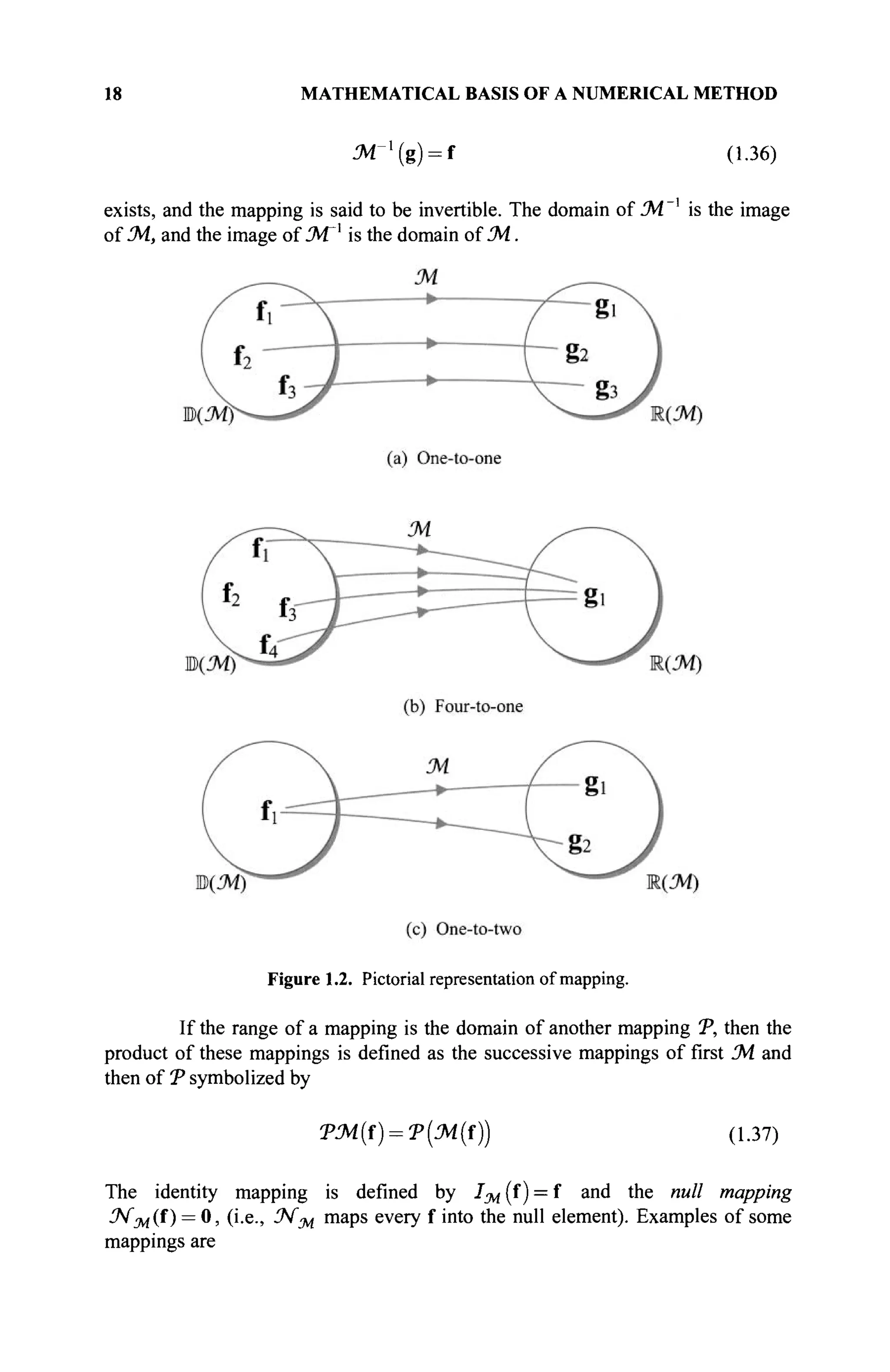
mapping is said to be into W. If 3i(f ) = g maps distinct elements f, into distinct
elements g„ then the mapping is said to be one-to-one. lin elements f, map into the
element g„ then the mapping is said to be n-to-one, and if each element f, maps
into n elements g„ then it is said to be one-to-n. These concepts are illustrated in
Figure 1.2.
If a mapping is one-to-one and onto W, then the inverse mapping](https://image.slidesharecdn.com/timeandfrequencydomainsolutionsofemproblemsusingintegralequationsandahybridmethodologyb-250205130750-568a5ba2/75/Time-and-Frequency-Domain-Solutions-of-EM-Problems-Using-Integral-Equations-and-a-Hybrid-Methodology-B-H-Jung-pdf-39-2048.jpg)
![MAPPING/TRANSFORMATION 19
function: f(x) = sinx —y (1.38)
functional: φ(ί)= I f(x)dx= I sm(x)dx = y (1-39)
M2
->R; M(x) = xl+2x2 =y (1.40)
; M{x) = X T ~T~ ^•X'i
X-2 Xl
= У2
(1.41)
A transformation Л is bounded on its domain, if for all u in Ш)(Л) there exists a
constant С such that [3]
И»И<с|Н1 (1.42)
Thus, the ratio of the "output" norm to the "input" norm is bounded. The smallest
number V that satisfies the inequality for all u in Ю(Л) is the norm of Л, written
as ||Λ||, and is defined as follows:
II „ II ΙΙ-ЯмЦ и „ ||
Л = sup V Î T = SU
P PH (1-43)
1-й HI I«H
The prefix "sup" implies supremum (i.e., the maximum value attained for any u).
Differential operators are not bounded, whereas the integral operators are bounded
[4, pp. 282-283].
A mapping L is linear if
£(af) = a£(f) and
(1 44)
£(f,+f2 ) = A + £ f 2
for all f and a. The null space, N^ of a mapping is the set {f,} such that
-£(f,) = 0. The null space of any linear mapping must contain the null element
f — 0. A linear mapping i o n a finite-dimensional linear space has an inverse if
and only if f = 0 is the only solution to £(f ) = 0.
An important property for differential operators is that they are usually
not invertible unless boundary conditions are specified. As an example, consider
the operator T) = d/dx and the space P" of polynomials of degree n — 1 or less. If
f is a constant a, then Of = da/dx = 0 and f is an element of the null space.
Therefore, T) is not of polynomials f(x) for which /(0) = 0 , and then D is
invertible. The procedure can be described in two equivalent ways:
(a) The boundary condition / ( 0 ) = 0 is a part of the definition of the
operator.
(b) The boundary condition / ( 0 ) = 0 restricts the domain of the operator.](https://image.slidesharecdn.com/timeandfrequencydomainsolutionsofemproblemsusingintegralequationsandahybridmethodologyb-250205130750-568a5ba2/75/Time-and-Frequency-Domain-Solutions-of-EM-Problems-Using-Integral-Equations-and-a-Hybrid-Methodology-B-H-Jung-pdf-41-2048.jpg)
![20 MATHEMATICAL BASIS OF A NUMERICAL METHOD
Even if JA is bounded, the supremum may not be attained for any element u. If
||Λ|| = 0, then JA is the zero operator. If JA is continuous at the origin, then it is
continuous on all of B(JA), and 1A is continuous if it is bounded. A linear
transformation SA into itself is characterized completely by its values through a
fixed basis h,, h2, · · ■, h . Indeed if we can write
u = ^ a r h and v = JAa = У^а,-Ah,·
j= j=
then the knowledge of и vectors JAb}, JAb2,..., JAhn enables us to calculate JAa
or v.
1.5.1 Representation by Matrices
Consider a linear mapping £ from a space W with elements f to a space G
resulting in elements g, that is, £(f ) = g. Let {fj, f2,..., f„} be a basis for W and
express an arbitrary element f in W as
Substitute this equation into the linear mapping g = £(f ) and obtain
(1.45)
g = £ [ / ] = £ Î>/f
/
;=1
:
Σ«/Α- (1.46)
Because every element in G can be written in this form, {£f,} must span G.
However, the {£ft} may be linearly dependent and, hence, may not form a basis
for G. We can obtain a basis {gi,g2,---,g„} for G from the {£fj} and express
the g in this basis as
g = Agi + ßi%2 +
and express each £ft in this basis as
ßn&r, (1.47)
Α=ΰίΐΐ8ΐ+α
2ΐ82+ ■■■+a
mZm
£f2 = 0,2g! + «22g2 + · · · + am2g„
A = a
l„8l + «2«82 + · · · + amng„
(1.48)
In terms of these matrices, one can write that [£l] is the column matrix of £ft,
[g] is the column matrix of g,, and](https://image.slidesharecdn.com/timeandfrequencydomainsolutionsofemproblemsusingintegralequationsandahybridmethodologyb-250205130750-568a5ba2/75/Time-and-Frequency-Domain-Solutions-of-EM-Problems-Using-Integral-Equations-and-a-Hybrid-Methodology-B-H-Jung-pdf-42-2048.jpg)
![MAPPING/TRANSFORMATION 21
[A]:
an au
a
2 a
22
a
m a
m2
*n
л
2п
(1.49)
Hence, one can write
[sT
ß]=[A]T
[g{[a] = [gT
[A[a (1.50)
This is valid for all [g]r
, and therefore, the coefficient vectors [a] and [ß] are
related by
[/>] = № ] (1.51)
Hence, for every linear mapping £(f) — g, we can find a matrix representation
[Λ][α] = [/?]. As there are infinitely many basis sets, hence, any linear mapping
£(f ) = g can be represented in infinite ways by the matrix equation [Λ][α] — [/?].
1.5.2 Linear Forms
A linear mapping from a space V to the scalar field ÎH or С is called a linear form
or linearfunctional. If V is the space of и-tuples 9Ί" or <£", then a linear iormjXx)
can be written as
_р(х) = сЛ+с2х2+-+спхп (1.52)
where cl,c2,...,cn are constants. In vector form, this can be written as follows:
J»(*) = [cfx (1.53)
[C]T
is the row vector of components c,.
If V is a space of function f(x) defined on the interval a < x < b, then a
commonly encountered linear form is
j>{f)= f"c(x)f{x)dx (1.54)
where c{x) is a fixed function.
More generally, a linear form can be written as](https://image.slidesharecdn.com/timeandfrequencydomainsolutionsofemproblemsusingintegralequationsandahybridmethodologyb-250205130750-568a5ba2/75/Time-and-Frequency-Domain-Solutions-of-EM-Problems-Using-Integral-Equations-and-a-Hybrid-Methodology-B-H-Jung-pdf-43-2048.jpg)
![22 MATHEMATICAL BASIS OF A NUMERICAL METHOD
Xf) = f*c{x)£(f{x))dc (1.55)
where £ is a linear operator.
Let M be a linear manifold in the separable complex Hubert space H (a
space that contains an orthonormal spanning set, or in other words, a basis exists
for that space). If to each u in M there corresponds a complex number, denoted by
£(u), satisfying the condition.
£(au + ß) = a£(vt) + ߣ(x) for all u, vin M (1.56α)
and for all complex numbers a, β. We say that £ is a linear functional in M. A
linear mnctional satisfies £(0) = 0 and
£ Î2a
ia
J = Èa
A»j) (1-566)
У=1
A linear functional is bounded on its domain M if there exists a constant
"U such that for all u in M, |£(u)| < TJ|ju||. The smallest constant "U for which this
inequality holds for all u in M is known as the norm of £ and is denoted by ||£||.
A linear functional continuous at the origin is also continuous across its
entire domain of definition M. Boundedness and continuity are equivalent for
linear functionals. A functional whose value at u is ||u|| is not linear. It is also of
interest to note that to each continuous linear functional £ defined on the space H
corresponds an unambiguously defined vector f such that
£(u) = (u,f) for every u in M (1.57)
1.5.3 Bilinear Forms
A mapping involving two elements, x in V] and y in V2 (V and V2 may be the
same space), to the scalar field Ü
H or € is called a bilinear form or a bilinear
functional if it is linear in each element. In other words, Л(х,у) is a bilinear form
if
Л(а1х1+а2х2,у) = а1Л(х1,у) + а2Л(х2,у) and (1.58)
Л(х,а1у1+а2у2) = щЯ(х,у1) + а2Л(х,у2) (1.59)
for all x and y. If Vi and V2 are complex spaces of и-tuples, then a bilinear form
can be written as](https://image.slidesharecdn.com/timeandfrequencydomainsolutionsofemproblemsusingintegralequationsandahybridmethodologyb-250205130750-568a5ba2/75/Time-and-Frequency-Domain-Solutions-of-EM-Problems-Using-Integral-Equations-and-a-Hybrid-Methodology-B-H-Jung-pdf-44-2048.jpg)
![THE ADJOINT OPERATOR 23
A(x,y) = [xf[A}[y} (1.60)
where [A] is a matrix and the superscript H denotes the conjugate transpose. Note
that if x is a constant, then JA(x, y) is a linear form in y, and if y is a constant,
then JA(x, у) is a linear form in x.
If Vi and V2 are function spaces, then a possible bilinear form in terms of
a single variable is
^(f,g) = fb
f{x)g{x)dx (1.61)
J a
More generally,/and g may be operated on by linear mappings. For example,
A(i,g) = fb
dxf{x)fb
g{x-y)dy (1.62)
О а О а
is a bilinear form. Again, note that if one function is kept constant, then the
bilinear form reduces to a linear form in the other function.
1.5.4 Quadratic Forms
If both arguments of a bilinear form A(x,y) are the same, then we obtain a
quadratic form or quadratic functional q(x) = JA(x, x). If x is an и-tuple, then the
general quadratic form is
q(x) = A(x,x) = [xf[A][x] (1.63)
obtained by setting x = y. Note that A must now be an x n matrix [A]. There is
no loss of generality if we also assume [A] to be symmetric.
If the argument of a quadratic form is a function, then we can also
construct a symmetric bilinear form associated with it. In general, we have
q(f + g) = A{t + g,f + g) = A(f,f) + A(t,g) + A(g,t) + A(<g,g) (1.64)
If it is specified that A(î,%) = A(g, f), then
^(f,g) = | ( i ( f + g ) - q ( f ) - i ( g ) ) (1.65)
1.6 THE ADJOINT OPERATOR
The adjoint operator Ά is defined by [3,4]](https://image.slidesharecdn.com/timeandfrequencydomainsolutionsofemproblemsusingintegralequationsandahybridmethodologyb-250205130750-568a5ba2/75/Time-and-Frequency-Domain-Solutions-of-EM-Problems-Using-Integral-Equations-and-a-Hybrid-Methodology-B-H-Jung-pdf-45-2048.jpg)
![24 MATHEMATICAL BASIS OF A NUMERICAL METHOD
(JZU,W) = ( W , ^ J ) (1.66)
for all ЗеШ(Л) and W e Ю(ЛЯ
). The operator Л is self-adjoint not only if
Я = JAH
but also requires ЩЛ) = ЩЛН
). If the two domains are not equal,
then the operator JA is called symmetric. The operator JA tells us how a system
will behave for a given external source. The adjoint operator, however, tells us
how the system responds to sources in general. Thus, the adjoint operator provides
physical insight into the system. An operator is said to be self-adjoint if
(Λχ,ζ) = (x,JAz) for all functions in the domain of JA. A self-adjoint operator is
said to be positive definite if (JAz, z) > 0 for z ^ 0.
For a differential operator, the adjoint boundary conditions are obtained
from the given operator and its given boundary conditions. For example, consider
the following second-order differential operator in the region between a and b [3,
4]:
JA= у with S,(M(x = a)) = a <ma Ъ1{и{х = Ъ)) = ß (1.67)
then we have from the definition of the adjoint operator
ь
f(wJAJ-JAH
w)dz = {'B(j,W)}b
a (1.68)
a
By equating the term (called the bilinear concomitant) [2?(J,W)]* = 0, one
obtains the adjoint boundary conditions for the given differential equation [3,4],
and the expression for the adjoint operator is given in terms of the expression
associated with JA .
For an integral operator, however, no adjoint boundary conditions are
required. For example, for the given integral operator
ь ь
x)u (x) dx
= Ju(x)dxJv(z)K(z,x)dx = (и,Лн
^
Hence, if the integral operator is a convolution operator (i.e., K(z,x) = z — x),
then the adjoint operator is the correlation operator. This subtle distinction is
significant as we will observe later on in Section 1.12 when one wishes to find the
convergence properties of a solution procedure.](https://image.slidesharecdn.com/timeandfrequencydomainsolutionsofemproblemsusingintegralequationsandahybridmethodologyb-250205130750-568a5ba2/75/Time-and-Frequency-Domain-Solutions-of-EM-Problems-Using-Integral-Equations-and-a-Hybrid-Methodology-B-H-Jung-pdf-46-2048.jpg)
![THE ADJOINT OPERATOR 25
Next we illustrate the interesting relationship between the domain and the
range of the operator and its adjoint, in particular, from the orthogonal
decomposition theorem [4],
ЩЛ) = П(Л)^ш(Лн
); and Ш>(Лн
) = п(Лн
)^Ш{Л) (1.70)
The symbol ^ denotes that these direct sums are orthogonal, and the only
common element between the two spaces is the null element. The overbar over the
two subspaces Ш(Л.) and М(ЛЯ
) indicates the completion of these two linear
manifolds. The two properties in Eq. (1.70) are illustrated in an abstract fashion by
Figure 1.3. Here, for example, М(ЛЯ
) denotes the null space of SAH
, (i.e., if
JAH
W = 0, then W G N(J4.W
)). It is thus clear from (1.70) and Figure 1.3 that
К ( Л ) с В ( Л я
) ( 1 . е , ЩЛ) is contained in Ώ(ΆΗ
)). In practice, usually it is
easier to find Ш(ЛН
) rather тапМ(Л). ЩЛН
) has a direct impact on the
existence of a solution to an operator equation JAf = g,(i.e., the solution to this
equation does not exist if g^D(Jz
l/ /
) ). The implication of this also will be
illustrated by the conditions that the weighting functions need to satisfy in the
solution of an operator equation by the method of moments. Next, we will look at
the properties of the operator equation.
Figure 1.3 Orthogonal direct sum decomposition generated by the operator and its adjoint
[4]. The only common element between the two orthogonal spaces is the null element.](https://image.slidesharecdn.com/timeandfrequencydomainsolutionsofemproblemsusingintegralequationsandahybridmethodologyb-250205130750-568a5ba2/75/Time-and-Frequency-Domain-Solutions-of-EM-Problems-Using-Integral-Equations-and-a-Hybrid-Methodology-B-H-Jung-pdf-47-2048.jpg)
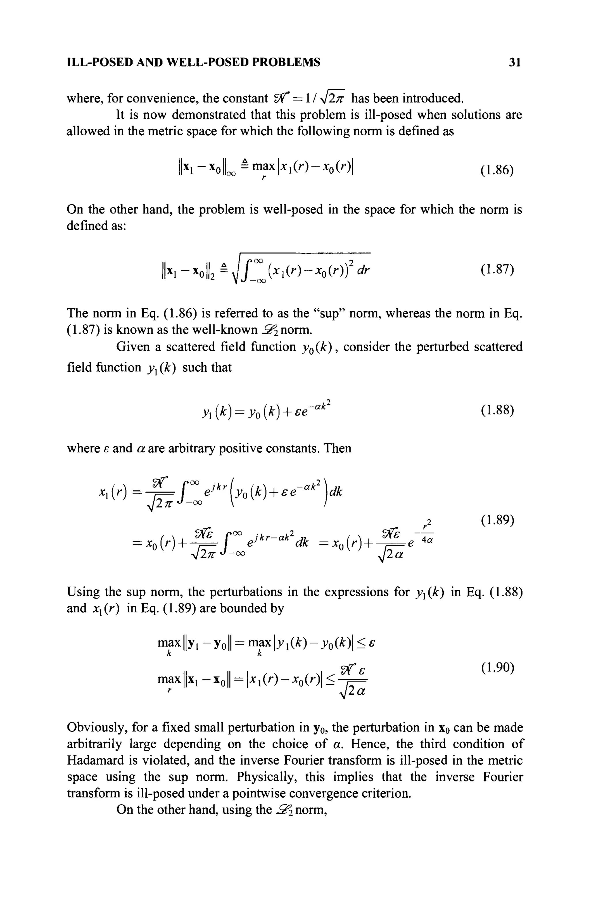
![ILL-POSED AND WELL-POSED PROBLEMS 27
If the input J. is bounded, that is,
|Л(0|<<7Й° (a constant) (1.76)
it follows that
У2-У1 <ЪЖ sin(i»r)i/r = l
- -—± (1.77)
Jo со
We conclude that
1
1 1
1 2х;
Ж
У2-У1 < (1-78)
ω
Obviously, by selecting ω to be sufficiently large, the difference y2 — yj can be
made arbitrarily small. The ill-posedness of this example is evidenced by the fact
that small differences in у can map into large differences in x. This issue poses a
serious problem because, in practice, measurement of у will be accompanied by a
nonzero measurement error (or representation error in a finite precision digital
system) δ. Use of the "noisy" data can yield a solution significantly different from
the desired solution.
When a problem is ill-posed, an attempt should be made to regularize the
problem. The solution to the regularized problem will be well-behaved and will
offer a reasonable approximation to the solution of the ill-posed problem.
The concepts of well-posed problems and the regularization of ill-posed
problems have been discussed in depth in the mathematical literature [5-12]. In
this section, we illustrate some of the significant concepts involved by means of
simple examples that arise in engineering applications.
1.7.1 Definition of a Well-Posed Problem
Hadamard [7,8] introduced the notion of a well-posed (correctly or properly
posed) problem in the early 1900s when he studied the Cauchy problem in
connection with the solution of Laplace's equation. He observed that the solution
x(t) did not depend continuously on the excitation y(t). Hadamard concluded
that something had to be wrong with the problem formulation because physical
solutions did not exhibit this type of discontinuous behavior. Other
mathematicians, such as Petrovsky, reached the same conclusion. As a result of
their investigations, a problem characterized by the equation J4x = у is defined to
be well-posed provided the following conditions are satisfied:
(1) The solution x exists for each element у in the range space Y; (this
implies that either К ( Л Я
) is empty or else any nontrivial solution of
JAH
= 0 , with v e М(ЛЯ
) should ensure v be orthogonal to y.](https://image.slidesharecdn.com/timeandfrequencydomainsolutionsofemproblemsusingintegralequationsandahybridmethodologyb-250205130750-568a5ba2/75/Time-and-Frequency-Domain-Solutions-of-EM-Problems-Using-Integral-Equations-and-a-Hybrid-Methodology-B-H-Jung-pdf-49-2048.jpg)
![28 MATHEMATICAL BASIS OF A NUMERICAL METHOD
(2) The solution x is unique; (This implies that Ν(Λ) is empty).
(3) Small perturbations in y result in small perturbations in the solution x
without the need to impose additional constraints.
If any of these conditions are violated, then the problem is said to be ill-posed.
Examples of ill-posed problems are now discussed. We first consider an example
in which condition (1) is violated.
Example 2
Suppose it is known that
y = x]tl+x2t2 (1.79)
In addition, assume that the observation y is contaminated by additive noise. The
observations and corresponding time instants are tabulated in Table 1.1.
TABLE 1.1. Data of Example 2
h 2 i i
h 1 2 3
Observation ofy(t) 3 3 5
Solution for x andx2 leads to the solution of the following matrix equation:
2 lj [3'
Л х = 1 2 ' = 3 (1.80)
Because Eq. (1.80) consists of three independent equations in two unknowns, a
solution does not exist. Condition (1) is violated, and the problem is ill-posed.
Example 3
Violation of condition (2) is illustrated by the following example. Observe
whether the operator SA in Eq. (1.71) is singular (i.e., the solutions of the equation
_Ях = 0 are nontrivial, and x * 0 ) , then Eq. (1.71) has multiple solutions. Such a
case occurs when one is interested in the analysis of electro-magnetic scattering
from a dielectric or conducting closed body at a particular frequency that
corresponds to one of the internal resonances of the body, using either only the
electric field or the magnetic field formulation.
The final example in this section illustrates a problem for which condition
(3) is violated.
Example 4
Consider the solution of the matrix equation [A][x] = [y] where [A] is
the 4 x 4 symmetric matrix of [13] as follows:
2 1
1 2
1 3
[x,
к =
3
3
5](https://image.slidesharecdn.com/timeandfrequencydomainsolutionsofemproblemsusingintegralequationsandahybridmethodologyb-250205130750-568a5ba2/75/Time-and-Frequency-Domain-Solutions-of-EM-Problems-Using-Integral-Equations-and-a-Hybrid-Methodology-B-H-Jung-pdf-50-2048.jpg)
![ILL-POSED AND WELL-POSED PROBLEMS 29
and
Mr
36.86243 51.23934 53.50338 50.49425
51.23934 71.22350 74.37005 70.18714
53.50338 74.37005 77.66275 73.29752
50.49425 70.18714 73.29752 69.17882
[192.09940 267.02003 278.83370 263.15773]
Wr
=[i i i i]
(1.81)
(1.82)
However, it can be shown that [A] is an ill-conditioned matrix in the sense that the
ratio of its maximum to minimum eigenvalues is on the order of 1018
.
Let us study the effect on the solution x, when only one component of y-, is
changed in the fifth decimal place. Specifically, we obtain the results presented in
Table 1.2. Clearly, extremely small perturbations in [y] result in large variations
in [x]. Condition (3) is violated, and the problem is ill-posed.
TABLE 1.2. Data of Example 4
[yf
[xf
[xf
yf
[xf
[y]r
[xf
192.09939 267.02003 278.83370 263.15773
-6,401,472,429 3,866,312,299 1,607,634,613 -953,521,374
192.09940 267.02002 278.83370 263.15773
3,866,312,299 -2,335,145,694 -970,966,842 575,900,539
192.09940 267.02003 278.83369 263.15773
1,607,634,615 -970,966,842 -403,733,529 239,462,717
192.09940 267.02003 278.83370 263.15772
-953,521,374 574,900,539 239,462,717 -142,030,294
1.7.2 Regularization of an Ill-Posed Problem
Most inverse problems of mathematical physics are ill-posed under the three
conditions of Hadamard. In a humorous vein, Stakgold [3, p. 308] pointed out that
there would likely be a sharp drop in the employment of mathematicians if this
were not the case.](https://image.slidesharecdn.com/timeandfrequencydomainsolutionsofemproblemsusingintegralequationsandahybridmethodologyb-250205130750-568a5ba2/75/Time-and-Frequency-Domain-Solutions-of-EM-Problems-Using-Integral-Equations-and-a-Hybrid-Methodology-B-H-Jung-pdf-51-2048.jpg)
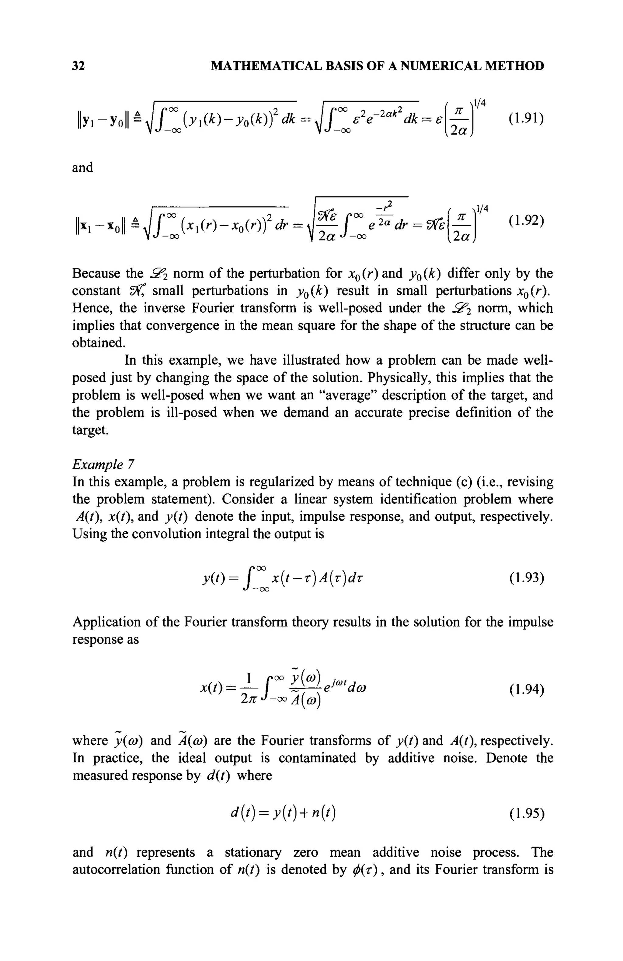
![30 MATHEMATICAL BASIS OF A NUMERICAL METHOD
Given an ill-posed problem various schemes are available for defining an
associated problem that is well-posed. This approach is referred to as
regularization of the ill-posed problem. In particular, an ill-posed problem may be
regularized by
(a) Changing the definition of what is meant by an acceptable solution
(b) Changing the space to which the acceptable solution belongs
(c) Revising the problem statement
(d) Introducing regularizing operators
(e) Introducing probabilistic concepts so as to obtain a stochastic extension
of the original deterministic problem
These techniques now are illustrated by a series of examples. Technique (a) is
demonstrated in Example 5.
Example 5
Once again, consider the problem introduced in Example 2. This resulted in Eq.
(1.80) for which a solution did not exist. Nevertheless, an approximate solution is
possible. One of several possible approximate solutions for any over-determined
linear system is the Moore Penrose generalized inverse [14], which is a least-
squares solution to Eq. (1.80) and is given by
<иГи"ь 0.8
1.3142
(1.83)
where the superscript H denotes the transpose conjugate of a matrix. Note that [x]
does not exactly satisfy any of the three equations in Eq. (1.80). Yet, [x] is a
reasonable approximate solution. We see that the original problem, which was ill-
posed because a classical solution did not exist, has been regularized by redefining
what is meant by an acceptable solution. Technique (b) is illustrated in Example 6.
Example 6
Relative to Lewis-Bojarski inverse scattering [15-17], the relationship at all
frequencies and aspects between the backscattered fields y(k) to the size and
shape of the target x(r) is given by
>{k)= f°° x{r)e~jkr
dr (1.84)
J —oo
This relation is valid under the assumption that the target currents are obtained
using a physical optics approximation. In Eq. (1.84), SA is the Fourier transform
operator. The solution to Eq. (1.84) is given by the inverse Fourier transform
(Г
) = 4 = Г y(k
>+Jkr
dk (1.85)](https://image.slidesharecdn.com/timeandfrequencydomainsolutionsofemproblemsusingintegralequationsandahybridmethodologyb-250205130750-568a5ba2/75/Time-and-Frequency-Domain-Solutions-of-EM-Problems-Using-Integral-Equations-and-a-Hybrid-Methodology-B-H-Jung-pdf-52-2048.jpg)
![ILL-POSED AND WELL-POSED PROBLEMS 33
denoted by φ(ω). When the measured noisy response d{t) is used in place of the
ideal output y(i), the solution x(t) becomes a random process. The variance of
x(t) is given by [18]
2 1 f00
~Φ{ω
) ,
This problem is considered to be well-posed only if σ is suitably small.
Typically, the noise is assumed to contain a background component of
white noise. With this assumption, the power spectral density φ{ώ) approaches a
nonzero constant K,, whereas ω approaches infinity. When σχ is infinite, the
problem becomes obviously ill-posed.
The problem can be made well-posed by revising the problem statement.
From a mathematical point of view, the input could be restricted to signals whose
Fourier transform Α{ώ) is a rational function with a numerator polynomial of a
higher degree than the denominator polynomial. Then, even with a white noise
background, σχ remains finite, and the problem becomes well-posed. However,
this regularization implies the presence in A(t) of singularity functions such as
impulses, doublets, and so on. Therefore, the regularization is achieved at the
expense of requiring A(t) to be an unrealizable signal having infinite energy.
A preferable approach is to remove the commonly used assumption of a
white noise background. Provided the power spectral density of the noise <j>{co)
falls off in frequency at a rate that is at least as fast as that of
р(й>)| ωχ+ε
(ε> 0, arbitrary)
σ will be finite. This demonstrates that the noise must be modeled carefully if the
problem is to be well-posed. This principle has direct implications in the solution
of time domain electromagnetic field problems.
Example 8
Technique (d), the application of regularizing operators, is discussed next. In
example 2, the three simultaneous equations were shown to be inconsistent, and
therefore, an exact solution did not exist. In example 5, an approximate solution
was obtained using the least-squares approach. The solution was given by Eq.
(1.83).
As the dimensionality of the problem is increased, there is a tendency for
the solution to oscillate and increase in magnitude. Therefore, the problem
becomes ill-posed as the dimensionality increases. This difficulty may be
overcome by introducing regularizing operators that impose additional constraints](https://image.slidesharecdn.com/timeandfrequencydomainsolutionsofemproblemsusingintegralequationsandahybridmethodologyb-250205130750-568a5ba2/75/Time-and-Frequency-Domain-Solutions-of-EM-Problems-Using-Integral-Equations-and-a-Hybrid-Methodology-B-H-Jung-pdf-55-2048.jpg)
![34 MATHEMATICAL BASIS OF A NUMERICAL METHOD
on the solution. In particular, instead of solving the problem JAx = y directly,
attention is focused on the problem of minimizing ||Άχ — y|| under the constraint
|A|| =τ
where £ is a suitably chosen linear operator. Equivalently, one finds
min|||j4x-y|2
+/i2
|2x|2
|
where μ plays the role of a Lagrange multiplier. If £ is the identity operator, then
this approach will result in that solution x, which carries out the minimization of
||-Ях - y|| having a specified value of||x|| . If £ is the derivative operator, then
this approach will result in that solution x, which carries out the minimization of
||Лх —y|| with a priori degree of smoothness for the solution (i.e., a specified
value of dx I dt ).
The parameter μ is determined by the constraint (e.g., the specified value
of ||x| , or the specified degree of smoothness or a combination of both) [8, chs. II,
III]. Many choices of the operator £ are possible, and one may simultaneously
apply several constraints with different corresponding Lagrange multipliers [8,
chs. II, III].
The solution of the problem posed in Eq. (1.71) is equivalent to the
solution of the matrix equation
[Af [Α + μ2
[Lf [Ц [x] = [Af [y] (1.97)
and is given by
[x] = [lAf[A] + M2
[L]H
[L]]~Af[y] (1.98)
This approach is known as the Tykhonov regularizing scheme [8,18,19]. Note, if
£ is the null operator (i.e., if no constraint is imposed), then the solution in (1.97)
reduces to the classical least-squares solution of (1.83). The Tykhonov
regularizing scheme has been used to regularize the ill-posed antenna pattern
synthesis problem and the image-processing problem [5].
The last approach to be discussed for regularizing an ill-posed problem is
through the application of technique (e). In this approach, a stochastic extension of
an otherwise deterministic problem is obtained by introducing probabilistic
concepts. Once again, consider the solution of JAx — y, where JA and у are](https://image.slidesharecdn.com/timeandfrequencydomainsolutionsofemproblemsusingintegralequationsandahybridmethodologyb-250205130750-568a5ba2/75/Time-and-Frequency-Domain-Solutions-of-EM-Problems-Using-Integral-Equations-and-a-Hybrid-Methodology-B-H-Jung-pdf-56-2048.jpg)
![NUMERICAL SOLUTION OF OPERATOR EQUATIONS 35
deterministic quantities. As mentioned previously, in some instances, perfect
measurement or observation of y is impossible. For those cases, the use of the
noisy measurements for y results in an ill-posed problem. With technique (e), the
problem is made well-posed by recognizing that uncertainty in the observation of
y causes uncertainty in the resulting solution for x. Consequently, the solution is
viewed as a random process. An error criterion is specified, and a stochastically
optimum solution is obtained. The solution is stochastically optimum in the sense
that repetition in measurements of y produces solutions for x, which on the
average, are optimum according to the specified error criterion. The details of this
approach are available in references [5,20,21].
1.8 NUMERICAL SOLUTION OF OPERATOR EQUATIONS
If it is assumed that the solution to (1.71) exists for the given excitation y, then
symbolically, the solution to (1.71) can be written as
х = Л_ 1
у (1.99)
Observe whether the operator Л is singular (i.e., the solutions of the equation
JAx = 0 are nontrivial, x ^ O ) because then (1.99) has multiple solutions. We
will assume, at the present moment, that such a situation does not develop. If one
is really interested in the analysis for the case when Άχ = 0 has a nontrivial
solution, then the present techniques can be modified to treat those special cases.
Finally, we assume JA.~l
is a bounded operator. This implies that small
perturbations of the excitation only produce a small perturbation of the solution as:
И^Цл^ЦЦуЦ (1.100)
where ||x|| defines either the Зг norm, 2C norm, or the S^ norm defined by;
jSf: | x | = rx(zfdz
2?. ||4= HUzidz (1.101)
_Sg: ||x|| = max x(z)
In the text, we will use only the mean square or the 2f2 norm because it is easy to
prove convergence of numerical techniques, even for discontinuous solutions.
In this section, we wish to solve the operator equation JAx - у = 0 . The
solution x is called a classical solution if (1.71) is satisfied everywhere in the
space § = В(Л). A generalized solution for x is the one that satisfies
(.Ях — у, φ) = 0 for all possible functions φ in a given class.](https://image.slidesharecdn.com/timeandfrequencydomainsolutionsofemproblemsusingintegralequationsandahybridmethodologyb-250205130750-568a5ba2/75/Time-and-Frequency-Domain-Solutions-of-EM-Problems-Using-Integral-Equations-and-a-Hybrid-Methodology-B-H-Jung-pdf-57-2048.jpg)
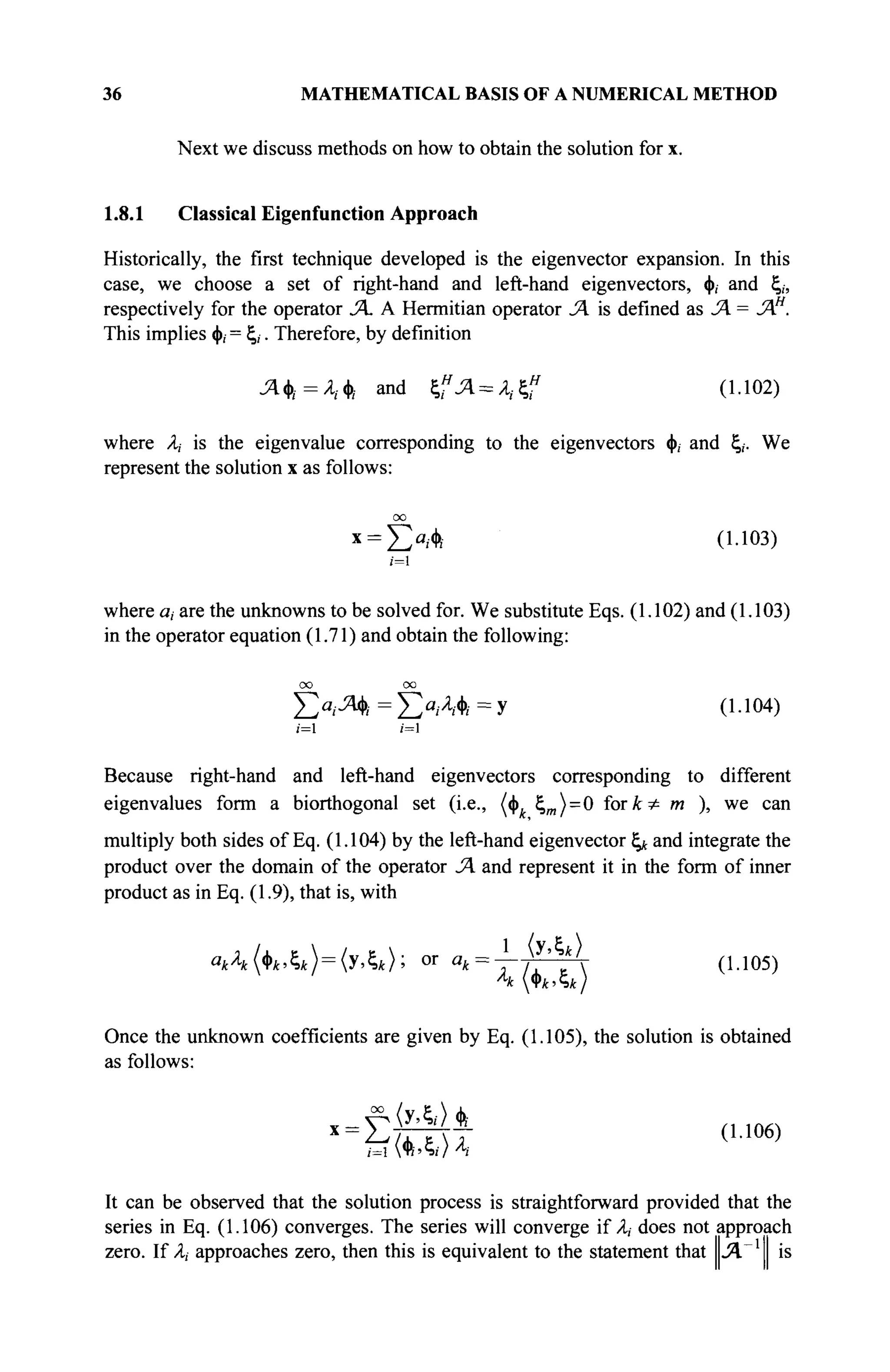
![NUMERICAL SOLUTION OF OPERATOR EQUATIONS 37
not bounded and the problem is ill-posed. This particular situation occurs when the
operator JA is an integral operator with a kernel К that is square integrable, that is,
P K(p,q)x(q)dq = y(p) ; with (1.107)
p dppK(p,qfdq< oo (1.108)
and p and q are variables of the kernel K. The major problem with Eq. (1.106) is
the determination of the eigenvectors. For simple geometries and other geometries
that conform to one of the separable coordinate systems, the eigenfunctions are
relatively easy to find. However, for arbitrary geometries, the determination of the
eigenvectors themselves is a formidable task. For this reason, we take recourse to
the computer for evaluating certain integrals and so on. Once we set the problem
up on a computer, we can no longer talk about an exact solution, as the computer
has only finite precision. The next generation of numerical techniques under the
generic name of method of moments (MoM) revolutionized the field of
computational electromagnetics. Problems that were difficult to solve by
eigenvector expansion and problems with arbitrary geometries now can be solved
with ease.
1.8.2 Method of Moments (MoM)
In the method of moments [22], we choose a set of expansion functions ψ,, which
need not be the eigenfunctions of JA We now expand the unknown solution x in
terms of these basis functions ψ, weighted by some unknown constants a, to be
solved for. So
N
χ « χ ^ = Σα,.ψ;. (1.109)
ι=1
The functions ψί need not be orthogonal. The only requirement on ψι is that we
know them precisely. By using the expression in Eq. (1.109), the solution to an
unknown functional equation of Eq. (1.71) is reduced to the solution of some
unknown constants in which the functional variations are known. This
significantly simplifies the problem from the solution of an unknown function to
the solution of a matrix equation with some unknown constants. The latter is a
much easier computational problem to handle in practice.
We now substitute Eq. (1.109) in Eq. (1.71) and obtain the following:
N
JAxKjAxN=Y^ciiJA?iKy (1.110)
/=i
This results in an equation error](https://image.slidesharecdn.com/timeandfrequencydomainsolutionsofemproblemsusingintegralequationsandahybridmethodologyb-250205130750-568a5ba2/75/Time-and-Frequency-Domain-Solutions-of-EM-Problems-Using-Integral-Equations-and-a-Hybrid-Methodology-B-H-Jung-pdf-59-2048.jpg)
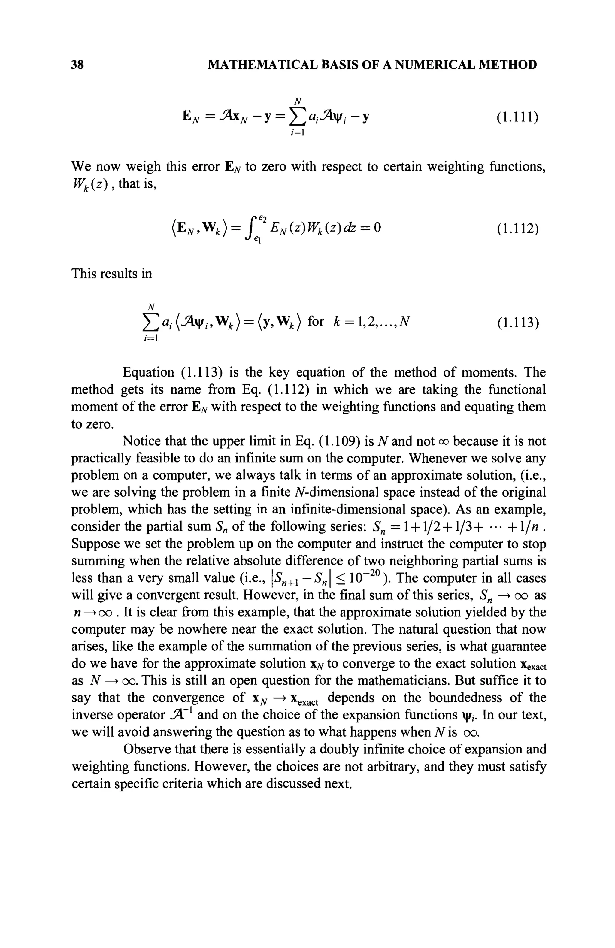
![NUMERICAL SOLUTION OF OPERATOR EQUATIONS 39
1.8.2.1 On the Choice of Expansion Functions. The expansion functions ψί
chosen for a particular problem have to satisfy the following criteria:
(1) The expansion functions should be in the domain of the operator Ρ(Λ) in
some sense, (i.e., they should satisfy the differentiability criterion and
must satisfy the boundary conditions for an integrodifferential operator
Л [23-28]). It is not at all necessary for each expansion function to
exactly satisfy the boundary conditions. What is required is that the total
solution must satisfy the boundary conditions at least in some
distributional sense. The same holds for the differentiability conditions.
When the boundary and the differentiability conditions are satisfied
exactly, we have a classical solution, and when the previous conditions
are satisfied in a distributional sense, we have a distributional solution.
(2) The expansion functions must be such that Λψ,, form a complete set for
i = 1,2,3,... for the range space К(_Я) of the operator. It really does not
matter whether the expansion functions are complete in the domain of the
operator; what is important is that Λψ; must be chosen in such a way
that Λψ, is complete, as is going to be shown later on. It is interesting to
note that when JA is a differential operator, ψ, have to be linearly
dependent for Λψ, to form a complete set. This is an absolute necessity,
as illustrated by the following example [23-28].
Example 9
Consider the solution to the following differential equation [23]:
- ■ ^ 4 ^ = 2 + sin(z) ΐοτΰ<ζ<2π (1.114)
dz1
with the boundary conditions: x(z = 0) = 0 = x(z = 2π). A normal choice for the
expansion functions would be to take sin(/z) for all i, that is,
*,<X> = ]Ta .sin(/z) (1.115)
/=1
These functions satisfy both the differentiability conditions and the boundary
conditions. Moreover, they are orthogonal. The previous choice of expansion
functions leads to the solution
x = x(z) = sin(z) (1.116)
It is clear that Eq. (1.116) does not satisfy Eq. (1.114), and, hence, is not the
solution. Where is the problem? Perhaps the problem may be that the functions
sin(z'z) do not form a complete set in Eq. (1.114) even though they are orthogonal](https://image.slidesharecdn.com/timeandfrequencydomainsolutionsofemproblemsusingintegralequationsandahybridmethodologyb-250205130750-568a5ba2/75/Time-and-Frequency-Domain-Solutions-of-EM-Problems-Using-Integral-Equations-and-a-Hybrid-Methodology-B-H-Jung-pdf-61-2048.jpg)
![40 MATHEMATICAL BASIS OF A NUMERICAL METHOD
in the interval [0,2л·]. Therefore, in addition to the sin terms we add the constant
and the cos terms in Eq. (1.115). This results in the following:
oo
x = x (z) = a0 + Σ {a
icos
(iz
) + b
isin
(iz
)) (1-117)
/=i
where a, and bh are the unknown constants to be solved for. Now the total solution
given by Eq. (1.117) has to satisfy the boundary conditions of Eq. (1.114).
Observe that Eq. (1.117) is the classical Fourier series solution, and hence, it is
complete in the interval [0,2л-
]. Now if we solve the problem again and choose
the weighting functions to be same as the basis functions, then we find the solution
still to be given by Eq. (1.115), and we know that it is not the correct solution.
What exactly is still incorrect? The problem is that even though a0, a, cosz'z, and
bt sin iz form a complete set for x, Λψ, (the operator JA operating on the
expansion function ψ,) do not form a complete set. This is because Λψ,, for
/ = 1,2,3,... are merely c, cos iz and c/, sin iz, where c, and dt are certain
constants. Note that from the set Λψ,, the constant term is missing. Therefore, the
representation of x given by Eq. (1.117) is not complete and, hence, does not
provide the correct solution.
From the previous discussion, it becomes clear that we ought to have the
constant term in Λψ,, which implies that the representation of x must be of the
following form:
oo
x = x(z) = Y^[ai cos (iz) + bj sin (iz)] + a0 +cz + dz2
(1.118)
i=l
and the boundary conditions in Eq. (1.114) have to be enforced on the total
solution. Observe that the expansion functions {1, z, z, sin (iz), and cos (iz)} in
the interval [0,2л·] and in the limit N —
> oo form a linearly dependent set. This is
because the set 1, sin(iz), and cos(iz) can represent any function such as z and z2
in the interval [0,2л·]. The final solution when using the expansion of (1.118) is
obtained as:
χ = χ(ζ) = ζ(2π-ζ) + ήη(ζ) (1.119)
which turns out to be the exact solution. This simple example illustrates the
mathematical subtleties that exist with the choice of expansion functions in the
MoM and hence the satisfaction of condition (2) by the basis functions described
earlier is essential.
1.8.2.2 On the Choice of Weighting Functions. It is important to point out that
the weighting functions W, (z) in the MoM have to satisfy certain conditions also](https://image.slidesharecdn.com/timeandfrequencydomainsolutionsofemproblemsusingintegralequationsandahybridmethodologyb-250205130750-568a5ba2/75/Time-and-Frequency-Domain-Solutions-of-EM-Problems-Using-Integral-Equations-and-a-Hybrid-Methodology-B-H-Jung-pdf-62-2048.jpg)
![NUMERICAL SOLUTION OF OPERATOR EQUATIONS 41
[23—28]. Because the weighting function weights the residual EN to zero, we have
the following:
(EN,VJ) = l^aiJ^l-y,y/J = (yN-y,yfj) = 0 (1.120)
As the difference уд, — у is made orthogonal to the weighting functions Wj(z), it
is clear that the weighting functions should be able to reproduce yN and to some
degree y.
From approximation theory [4,24—28], it can be shown using the
development of projection theory of section 1.4 that, for a unique minimum norm
representation, yN must be orthogonal to the error у — уд, as shown abstractly in
Figure 1.4. By Eq. (1.120), the weighting functions W, are also enforced to be
orthogonal to y - y w , and because they are not orthogonal to yN, it follows that
the weighting functions should be able to reproduce yN and to some degree y.
Figure 1.4. Best approximation of у by yN.
To recapitulate, in Eq. (1.71) the operator JA maps the elements x from
the domain of JA denoted by I$(JA) to the elements у in the range of JA, denoted
by R(J4.). This been depicted in Figure 1.3. Because the objective is to solve for
x, which is approximated by a linear combination of the expansion functions {ψ,}
for i = 1,2,..., N , it is clear that the expansion functions need to be in M(JA).
Only then can the expansion functions represent any element xN in M(JA). Then,
by definition
у*=Ёа
Л о·121
)
is in R(JA) because it is obtained by applying JA to xN, and the set Λψ, must
span Μ(Λ) , as any yN in R(J4.) can be written as a linear combination of
{.Αψ,}. It is the duty of the weighting functions W*to make the difference у - yN
small.
Also, as the weighting functions approximate yN, they must be in the
range of the operator. In other words, the weighting functions must form a basis in
the range of the operator, and in the limit N —
> oo must be able to represent any](https://image.slidesharecdn.com/timeandfrequencydomainsolutionsofemproblemsusingintegralequationsandahybridmethodologyb-250205130750-568a5ba2/75/Time-and-Frequency-Domain-Solutions-of-EM-Problems-Using-Integral-Equations-and-a-Hybrid-Methodology-B-H-Jung-pdf-63-2048.jpg)
![42 MATHEMATICAL BASIS OF A NUMERICAL METHOD
excitation y. When the weighting functions W* cannot approximate y to a high
degree of accuracy, the solution x# obtained by the technique of minimizing the
residuals may not produce a solution that resembles the true solution. Any method
that enforces the inner product to zero in Eq. (1.120) must satisfy the previous
criterion. In short, it is seen by relating (yN — y, W^ ) = 0 in Eq. (1.120) to the
theory of functional approximations that
(a) The weighting function W* must be in the range of the operator or, more
generally, in the domain of the adjoint operator.
(b) Because the weighting functions are orthogonal to the error of the
approximation, the set {Wk} should span yN.
(c) As N —» oo, yN -» y. Therefore, the weighting function should be able to
represent the excitation y in the limit.
If the weighting functions do not satisfy all of these criterions, then a meaningful
solution may not be obtained by the method of moments. Hence, if the weighting
functions are not in ЩУ.Н
), then they cannot be in К(Л). Therefore, to have a
meaningful result, the weighting functions must necessarily be in M(JAH
). It is
also clear from Figure 1.3 that if у of Eq. (1.71) is not an element ЩЛ.Н
), then
Eq. (1.71) does not possess any classical mathematical solution whatsoever. This
also precludes the existence of even a least-squares solution because, in this case,
the equivalent problem of JAH
JAx = Лн
у is solved, and if у is not in
В(ЛЯ
), then J4H
y is not mathematically defined. However, one could still find
a solution numerically, in which the solution will diverge as shown from a
mathematical point of view in [4,24-28]. In numerical electromagnetics, this
situation occurs when one solves a radiation problem with a delta gap excitation.
In this case, the solution seems to converge initially, but as more and more
expansion (basis) functions are chosen, ultimately, the solution seems to diverge.
This type of convergence is known as asymptotic convergence [29].
There are three different variations of the method of moments depending
on the choice of the testing functions. When Wk (z) = Sk (z), a delta function, we
obtain the point matching method. When Wk(z) = iyk(z), we obtain the Galerkin's
method. And finally, when Wk (z) = ^Αψίί (ζ), we obtain the method of least
squares. They are special cases of the more general method of minimizing
residuals [22-28].
1.9 DEVELOPMENTS OF THE VARIATIONAL METHOD
(RAYLEIGH-RITZ), GALERKIN'S METHOD, AND THE
METHOD OF LEAST SQUARES
So, in the present discussions, we assume that the operator equation in Eq. (1.71)
is well posed. Next, we investigate the nature of the solution yielded by the three
techniques—variâtional method (Rayleigh-Ritz), Galerkin's method, and the](https://image.slidesharecdn.com/timeandfrequencydomainsolutionsofemproblemsusingintegralequationsandahybridmethodologyb-250205130750-568a5ba2/75/Time-and-Frequency-Domain-Solutions-of-EM-Problems-Using-Integral-Equations-and-a-Hybrid-Methodology-B-H-Jung-pdf-64-2048.jpg)
![VARIATIONAL, GALERKIN'S AND LEAST SQUARE METHOD 43
method of least squares. We also present the conditions under which the three
techniques yield meaningful results and discuss their rates of convergence.
These three techniques proceed by assuming the nature of the solution a
priori in terms of known expansion functions. They start with the idea that the
approximate solution xN of x can be expressed in the following form:
N
x
*=EXu
» о·122
)
и=1
where a„ are certain unknown constants to be solved for. The expansion functions
u„ are a complete set of functions in an /V-dimensional space. In other words, the
sequence {u„} for n = 1, 2,..., N is a linearly independent set and thereby forms
a basis for the /V-dimensional space in which the approximate solution yN is
sought. It is not necessary that {u„} for n = ,2,...,N form an orthogonal set of
functions. The exact solution
oo
x
= Ea
«u
« (1123)
n=
lies in an infinite dimensional space. In summary, by the term convergence, then,
we imply convergence in the mean, Цхд, — x|| —
> 0 as N —> oo (i.e., in the limit N
approaches infinity), the mean-squared difference between х# and x approaches
zero. In the remaining sections, we discuss the restrictions that each of the three
methods impose on the expansion functions u„ and how an approximate solution
XJV is obtained. We also address the question of convergence of (Хд, — x) —
» 0 as
T
V —
» oo for the three methods. It is important to note that there are four different
types of convergence. They are [3]:
(1) Uniform convergence {pointwise convergence implies that, given a fixed
ε > 0, we can find a number N such that the absolute value
x(z)-xN(z)<£ for all z e [a,b] (1-124)
(2) Strong convergence (convergence in the norm or convergence in the
mean) implies
||x - Хд, || < £
■ ; thatis, Jj (x(z)-xN(z)f dz <ε (1.125)
(3) Convergence in energy requires that
(Ά(-χΝ),(χ-χΝ))<ε (1.126)](https://image.slidesharecdn.com/timeandfrequencydomainsolutionsofemproblemsusingintegralequationsandahybridmethodologyb-250205130750-568a5ba2/75/Time-and-Frequency-Domain-Solutions-of-EM-Problems-Using-Integral-Equations-and-a-Hybrid-Methodology-B-H-Jung-pdf-65-2048.jpg)
![44 MATHEMATICAL BASIS OF A NUMERICAL METHOD
in some physical problems represents energy, hence the name
energy norm, whereas convergence in the mean implies that the
converging sequence XJV may not approach the limit function x at every
point in the domain of JA, but the region in which the converging
sequence xN differs from x becomes arbitrarily small, as N —> oo.
Convergence in energy implies similar things happen to the derivative of
the sequence as well. This convergence only can occur for a positive
definite operator JA.
(4) Weak convergence {convergence in a distributional sense) implies that yN
converges weakly to x if
lim (χ^,φ) = (χ,φ)
N—*oo
(1.127)
or all φ in the space. The method of moments often yields solutions
that converge weakly to a generalized solution.
Finally, a set of functions u, is said to be complete in a space if any
function x in that space can be expanded in terms of the set {u,}, so that
x
-£a
/u
i <ε
A set of functions is said to be complete in energy if
и ι=1 J I /=1
<ε
for a positive definite operator JA.
1.9.1 Variational Method (Rayleigh-Ritz)
In the variational method, the solution to Eq. (1.71) is attempted by minimizing
the functional F(z) defined by [23-25, 30-33]
F(z) = (^z,z)-(y,z)-(z,y) (1.128)
In Eq. (1.128), it is assumed that the operator Л is a self-adjoint operator {i.e.,
JA = JAH
(adjoint operator) and ЩЛ) = ЩЛН
) }. So, by definition, a self-
adjoint operator satisfies the following equality: (Jfo,z) = (x, JAz). For non-self-
adjoint operators, J^.and у in Eq. (1.128) may be replaced by JA JA and JAH
y ,
respectively, and the following discussion still holds. The technique then becomes
the method of least squares. Assume that z is the estimated solution and x is the
exact solution of JAx = y. Now observe that Eq. (1.128) can be rewritten as](https://image.slidesharecdn.com/timeandfrequencydomainsolutionsofemproblemsusingintegralequationsandahybridmethodologyb-250205130750-568a5ba2/75/Time-and-Frequency-Domain-Solutions-of-EM-Problems-Using-Integral-Equations-and-a-Hybrid-Methodology-B-H-Jung-pdf-66-2048.jpg)
![VARIATIONAL, GALERKIN'S AND LEAST SQUARE METHOD 45
F(z) = (jzi(z-x),(z-x))-(y,x) (1.129)
Because (y, x) is a constant, minimization of ψ{τ) directly implies minimization
of ||z - x|| if and only if the operator JA is positive definite. It is thus clear that, for
an operator to be positive definite, it has to be self-adjoint first. This is because
| | ζ - χ | 2
< ( Λ ( ζ - χ ) , ( ζ - χ ) ) (1.130)
This is the philosophy behind solving Eq. (1.71) in a roundabout fashion by
minimizing the functional F(z) of Eq. (1.128).
We now replace z in Eq. (1.128) with xN (as defined in Eq. (1.122)) to
obtain
IN N / N / N
F(x
w)=(Ea
«^u
«>Ew-(y>Ea
«u
«MEa
;u
/'y) 0-131)
We solve for the unknowns a„ by minimizing F(xN) of Eq. (1.131). This is
achieved by taking the partial derivatives for df:
(xN)/daj for i = ,2,...,N and
equating each of the partial derivatives to zero. This results in a set of equations
N
£>и (Ли„,и,)-(у,и,) for к = 1,2,..., N (1.132)
и=1
The unknowns a„ are solved from Eq. (1.132). In the following subsections, we
develop the finer structures and limitations of this technique.
1.9.1.1 Does a Functional F(z) Always Exist? According to [3,23,25], the
solution x of a boundary value problem can also be characterized as the element
for which a related functional F(z) is stationary. Such a stationary characterization
is a variational principle whose Euler-Lagrange equation is the differential
equation of the original boundary value problem. The variational problem may
also provide guidance to the existence of a solution for the boundary value
problem.
If JAx = у has a solution x0, then this solution minimizes the functional
F(z) (as defined in equation (1.128)). Conversely, if an element x0 e B(JA) exists
that minimizes the functional F(z), then x0 satisfies JAx = y. This method of
solving a boundary value problem that consists of replacing JAx = у with the
problem of minimizing a functional F(z) is also called the energy method (as it
minimizes the energy of the system). This implies that a variational method finds a
solution with finite energy, or mathematically (y,x0) or (_Ях0,х0) is bounded.
As a first example, consider the self-adjoint operator jA as](https://image.slidesharecdn.com/timeandfrequencydomainsolutionsofemproblemsusingintegralequationsandahybridmethodologyb-250205130750-568a5ba2/75/Time-and-Frequency-Domain-Solutions-of-EM-Problems-Using-Integral-Equations-and-a-Hybrid-Methodology-B-H-Jung-pdf-67-2048.jpg)
![46 MATHEMATICAL BASIS OF A NUMERICAL METHOD
d2
x(z)
dz2
with x(z = 0) = 0 and x(z = 1) = 0 . It has been shown in reference [24] that this
operator is positive definite and, hence, has a bounded inverse. Moreover, the
homogeneous equation has the trivial solution. Now if we select
у = y(z) = —0.25z~3
' , then the exact solution is given by x = x(z) = z — y/z .
We observe ψ(ζ) —> oo as
<y,x> = /
о
Hence, the variational method is defined only for a class of problems in which
(y,x) and (у,Хдг) are bounded.
The discussion so far does not address the question of the existence of the
functional p(z) nor does it show how a solution x0 can be obtained. However,
such information may be obtained if the operator JA is positive/negative definite or
for a semi-definite operator if (x0,y) is bounded. In both cases, it is assumed that
у is square integrable. Thus, if (x0,y) is unbounded, then a variational method
cannot be set up for the solution of JAx = у , as the functional F(z) become
infinite. This is true for any self-adjoint operator.
As an analogy, consider the vector electric field E. Can this electric field
E always be derived from a scalar potential function V? If the curl of the vector is
zero (i.e., VxE = 0 ), then only the vector can be represented in terms of a
potential (i.e., E = W ). When the curl is zero, the integral of E along a path in
space Z is independent of the actual path taken and depends only on the end points
z and z2, that is,
ΓΖ2
Ε·ίώ = Κ,-Κ,
This provides an equivalent method of determining whether a vector field can be
derived from a scalar potential. So, from these elementary concepts of vector
calculus, it follows that if we regard the Euler equation in a variational method as
the gradient of a functional p(z) analogous to a potential, then we should not
expect every operator equation to be derivable from a potential independent of the
path integral.
Consider again the second-order differential operator given by the last
example. We know that the domain of the operator Ю(Л) consists of the space of
twice differentiable and square integrable functions that satisfy the boundary
conditions. Now if we consider the solution to JAx = y, in which JA is the second
order differential operator and у is a square integrable function, then our starting
point for solution is F(z), as given by Eq. (1.123). In this case, p(z) is bounded
below on B(JA) so that f(z) has a minimum, say p, on M(JA). If there is an
element x0 еЩЛ), for which f(x0) = p , then the infinimum is attained on
. - 1 - 5
(z — [z)dz —>oo .](https://image.slidesharecdn.com/timeandfrequencydomainsolutionsofemproblemsusingintegralequationsandahybridmethodologyb-250205130750-568a5ba2/75/Time-and-Frequency-Domain-Solutions-of-EM-Problems-Using-Integral-Equations-and-a-Hybrid-Methodology-B-H-Jung-pdf-68-2048.jpg)
![VARIATIONAL, GALERKIN'S AND LEAST SQUARE METHOD 47
M(SA) so that the problem for minimizing F(z) on ЩЛ) has the solution x0.
There are two reasons for considering the minimum of F(z) on a larger domain
M (as yet unspecified). First, Т{г) may not have a minimum on ЩЛ). If у is
only piecewise continuous and if SA is defined by the second-order differential
operator of the last example, then the solution x0 to SAx = у may not be in the
space of square integrable, twice differentiable functions so that SAx = у has no
solution. Hence, p(z) does not have a minimum on ©(Л). The trouble here is
simply that M(SA) is not a suitable domain on which to analyze the boundary
value problem when у is not continuous. The second reason is more subtle. Even if
p(z) has a minimum on ЩЛ), it may be hard to prove the fact directly. It turns
out to be easier to prove the existence of a minimum on the larger domain M and
then to show that the minimizing element lies in Ш)(Л). Thus, we shall try to
enlarge H(SA) so that the minimum for p(z) can be guaranteed to be in the new
domain. It is reasonable to hope for such an existence because the expression for
F(z) involves only the first derivative of x(z), whereas an element of b{SA) has
a continuous derivative of order 2.
We now complete M(SA) to form the larger domain M. This is achieved by
completing B(SA) with respect to a new inner product (x, х)л = (SAx, x) with
x G M. The completion of ЩЛ) with respect to this inner product results in a
new domain N. Thus, all elements of M are with finite energy as (Λχ,χ) is
bounded. If the operator SA is positive definite, then all elements of M satisfy
(Λι,χ) > ΤΓ2
(χ,χ) = "G2
[|x| where "U is a predetermined positive constant.
Therefore, for a positive-definite operator, the following inequality holds:
„ l|2 , . (SAx,x) (x,x)„
II II / ^ - 2 %2
and all elements of M are in ЩЛ). But in general, M is larger than Ώ(Ά). Now
we investigate the conditions for the existence of the functional F(z) on M. For a
positive-definite operator,
I
I II2
(x,y)2
< ||y||2
x|H|2
< И - ( Л х , ж ) for x e M (1.133)
holds for any square integrable function y, and (x,y) is always bounded on M.
Thus, the variational method exists for a positive-definite operator, and the
operator equation has a solution for any square integrable function.
However, when SA is semi-definite, inequalities like Eq. (1.133) do not
exist. Hence, for the variational method to exist, it is required that (x,y) be
bounded for a functional F(z) to exist.
Because (x,y) is now bounded, according to reference [3] a unique
element u0 e M exists such that (x,y) = (x,SAx0) for x e M . This element x0
also minimizes the functional F(z), and the minimum value is given by
Ί-(χ0) = —(x0,x0) = —(SAx0,x0). For a positive-definite operator, it is also](https://image.slidesharecdn.com/timeandfrequencydomainsolutionsofemproblemsusingintegralequationsandahybridmethodologyb-250205130750-568a5ba2/75/Time-and-Frequency-Domain-Solutions-of-EM-Problems-Using-Integral-Equations-and-a-Hybrid-Methodology-B-H-Jung-pdf-69-2048.jpg)
![VARIATIONAL, GALERKIN'S AND LEAST SQUARE METHOD 49
1.9.1.2 Does Minimization of T(N ) Lead to a Monotonie Convergence of the
Approximate Solution xN to the Exact One? The answer is yes, only if Л is a
positive/negative-definite operator. Otherwise, there is no guarantee that the error
in the solution Цхд, — x|| becomes smaller as the order of the approximation is
increased. We illustrate this by an example.
Example 10
Consider the solution of the following 3x3 matrix equation:
(1.136)
In this problem, JA is the 3x3 square matrix and у is the 3x1 column matrix. We
would like to obtain an approximate solution xN by the variational method. Of
course, when N = 3, we should get the exact solution of Eq. (1.136). In this
problem, we study the nature of the various orders of approximations to the
solution. By the terms of the problem, we form the functional
-4 2
3 6
6 2
X,
x2
X
3
=
1
5
10
T{x) = x X2 ^}]^'
X,
x2
x3
-2[xx x2 x3J
1
5
10
(1.137)
= 3xx — 8X[X2 + 3x2 + 4x]X3 + 12x2x3 + 2x3
2
— 2xj — 10x2 — 20x3
We now choose the expansion functions u„ (orthonormal) as
uf=[l 0 Of uf=[0 1 Of u [ = [ 0 0 if (1.138)
We now seek the first approximate solution to x as xf = axaT
x = ax 0 0] and
solve for X| by the variational method by using Eq. (1.132) to obtain
x,r
= [1/3 0 0] . Because the exact solution to the problem is x, = 1 for
/ = 1, 2,3 , the error in the solution is
X —X, 7(l-l/3)2
+(l-0)2
+(l-0)2
=1.56
We now solve for x2, which is the second-order approximation to x. So
x£=a,uf +a2uT
2=[ax 0 of + [0 a2 of = [ax a2 of (1.139)](https://image.slidesharecdn.com/timeandfrequencydomainsolutionsofemproblemsusingintegralequationsandahybridmethodologyb-250205130750-568a5ba2/75/Time-and-Frequency-Domain-Solutions-of-EM-Problems-Using-Integral-Equations-and-a-Hybrid-Methodology-B-H-Jung-pdf-71-2048.jpg)
![50 MATHEMATICAL BASIS OF A NUMERICAL METHOD
and we obtain the solution for x2 by using Eq. (1.132) as
X2 = [-23/7 - 1 9 / 7 0]T
. Observe that the error in the solution for the second-
order approximation is
||x - x21 = 7(l-23/7)2
+(l-19/7)2
+(l-0)2
= 5.76
By comparing ||x — x21| with ||x — x;11|, it is clear that there is a 269% increase in the
value of the error as the order of the approximation has been increased from
N = 1 to N = 2. Also, note that the residuals JAxl - y|| = 11.28 and
|J4X] — У||=
32.86 do not decrease either as N increases. However, when N = 3,
we would obtain the exact solution.
The error in the solution increases as we increased the order of the
approximation because JA is not a positive-definite matrix even though Л | is
bounded. So, if in a problem, the operator JA is self-adjoint but not positive
definite, then the variational method will not yield a more accurate answer, as the
order of the approximation is increased. Only for the solution of a scalar problem
of charge distribution on a wire or a plate caused by a constant potential, is the
operator self-adjoint and semi-definite. In almost all other cases, JA is a complex
symmetric operator. Hence, unless we have an operator that is positive definite,
increasing the order of the approximation in a variational method may not yield a
more accurate solution.
It is important to point out that the symmetric inner product is a mere
mathematical artifact and does not give rise to a natural definition of the norm.
Also, one cannot comment on the eigenvalues of a complex symmetric operator.
The symmetric product is more akin to the definition of reciprocity, and the
normal inner product is related to the definition of power, which is a physical
quantity. Thus by using the symmetric product, it is very difficult to comment on
the properties of the operator, as a symmetric product naturally does not give rise
to a norm, and hence, one cannot talk about convergence.
1.9.1.3 What Are the Restrictions on the Expansion Functions u„? The
expansion functions need not be in the domain of the operator. However, it is
essential that the expansion functions form a complete set with respect to the
following inner product (jAu^u A At is totally immaterial whether the expansion
functions form a complete set with respect to the inner product (u(-,u -j.For a
positive-definite-second-order differential operator -Д physically the previous
requirements imply that the expansion functions must be capable of representing
the solution x, as well as its first derivative. Thus, the expansion functions need
not be required to approximate the second derivative of the solution x. This
principle has been illustrated with an example in the Section 1.9.1.2 on the choice
of expansion functions.](https://image.slidesharecdn.com/timeandfrequencydomainsolutionsofemproblemsusingintegralequationsandahybridmethodologyb-250205130750-568a5ba2/75/Time-and-Frequency-Domain-Solutions-of-EM-Problems-Using-Integral-Equations-and-a-Hybrid-Methodology-B-H-Jung-pdf-72-2048.jpg)
![VARIATIONAL, GALERKIN'S AND LEAST SQUARE METHOD 51
1.9.1.4 Does Minimization of the Functional T(xN) Guarantee the
Convergence of the Residuals? The question can be restated mathematically as
follows: We know that when the operator Ά is positive definite and
F(x#+i) <F(XJV)» then we have ||x —хж+1|| <||х-Хд,| . Does this imply
И**+ 1 -У||<И**-У|?
The answer is that there is no guarantee whatsoever that the above
inequality would be satisfied. In fact, it is not even certain that the residuals will
decrease to zero as N increases. This is because in defining the expansion
functions u„, we have not specified that they belong to the domain of the operator.
If the expansion functions do not belong to the domain of the operator, then they
do not satisfy all the boundary conditions and the requisite number of
differentiability conditions for the problem. Hence, if u„ e В (Л), then J4.u„,and
hence, AuN lacks any meaning. So, in a variational method, it is not at all
necessary that
lim ILAu^-ylUO
N—>oc
If Л is a second-order differential operator, then what the variational method
guarantees is a solution such that the solution xN and its first derivative converge in
the mean to the exact solution x and its derivative x', respectively, as JV —
> oo.
II
However, the second derivative xN may not converge to x" in any sense.
However, if the sequences JAun are bounded, then it can be shown [24,25,30-32]
that the residual JAxN - у converges weakly to zero, in which the definition of
weak convergence is given by Eq. (1.127).
1.9.1.5 Epilogue Observe that, in the previous sections, we have talked of
convergence with respect to the norm defined by Eq. (1.125) (i.e., convergence in
the mean). Thus, the class of problems for which the convergence of a variational
method is mathematically justified is the class of problems that has a square
integrable solution x. The problems then for which the convergence of a
variational method cannot be physically or mathematically justified are the charge
distribution on a rectangular plate, the current distribution on an open-ended
cylinder irradiated by a plane wave, and so on. These are problems that do not
have a square integrable solution, as one component of the current has a square
root singularity.
However, a variational method may be extended to problems that do not
have a square integrable solution x by redefining the inner product in Eq. (1.9)
with Eq. (1.11) as
( u
; ' u
t ) w â
X w(z)M,(z)^(z)ufe
where w(z) is generally a nonnegative weight function. If we find a solution
xN(z) with the previously redefined inner product, then we know from the
previous discussions that we cannot guarantee that either of the two conditions,](https://image.slidesharecdn.com/timeandfrequencydomainsolutionsofemproblemsusingintegralequationsandahybridmethodologyb-250205130750-568a5ba2/75/Time-and-Frequency-Domain-Solutions-of-EM-Problems-Using-Integral-Equations-and-a-Hybrid-Methodology-B-H-Jung-pdf-73-2048.jpg)
![52 MATHEMATICAL BASIS OF A NUMERICAL METHOD
lim I (iN(z) — x(z)) dz —>0and lim I (JAxN(z)-y{zj) dz —» 0
will be satisfied. So, the application of a variational method to a problem with
non-square integrable solutions with the redefined inner product may yield a
mathematical solution that may not have any correlation to the actual physical
problem.
The other important point to remember is that, in a variational method,
we minimize the functional T{z) in Eq. (1.128). Moreover, we have not chosen
the expansion functions to be in the domain of the operator (i.e., satisfy both the
differentiability conditions and the boundary conditions). So there may be a
possibility that the element Uo, which minimizes the functional F(z), may not even
be in the domain of the operator. This often happens [23]. Under those
circumstances, the solution obtained by a variational method is called the
generalized solution to the problem. (A generalized solution is one that obeys
(φ, ΛχΝ - y) = 0 for all possible φ in a given class.)
In summary, the crux of a variational method lies in setting up the
functional p(z), as it may not always exist. The proper selection of a complete set
of expansion functions u„ is very important. Because the expansion functions need
not be in the domain of the operator, there is no guarantee that
lim Ц-Ях« — yll —
*
· 0
JV-^co" "
If F(xN ) exists, then
lim Цхд, — xll—>0
if and only if (y,x) and (y,xN) are bounded for all N
1.9.2 Galerkin's Method
In Galerkin's method, we select a complete set of expansion functions {u„} that
are in the domain of the operator, to approximate xN in Eq. (1.122). This implies
that the set {un} satisfies not only all the boundary conditions but also the
differentiability conditions of the problem. We now substitute Eq. (1.122) in Eq.
(1.71) to form
N
£ ^ u , = y (1.140)
(=1
Now J^u, means u, e ©(J4.). Next the residual](https://image.slidesharecdn.com/timeandfrequencydomainsolutionsofemproblemsusingintegralequationsandahybridmethodologyb-250205130750-568a5ba2/75/Time-and-Frequency-Domain-Solutions-of-EM-Problems-Using-Integral-Equations-and-a-Hybrid-Methodology-B-H-Jung-pdf-74-2048.jpg)
![VARIATIONAL, GALERKIN'S AND LEAST SQUARE METHOD 53
N
ι=1
is formed, and it is equated to zero with respect to the functions uk,
k = l,2,---,N. This yields a set of equations [23-31 ]
л £ а , . и ; , и Л = (у,иА), k = l,2,-,N (1.141)
Observe that, in Eq. (1.141), JA can even be nonlinear and non-self-adjoint. A
variational formulation for a nonlinear operator is complex. When JA is a linear
operator, Eq. (1.141) simplifies to
Σ Χ Λ Β , . , Ι Ι , Η Υ , Ι Ι * ) , k = l,2,-,N
/=i U-l4
A)
or [G][a] = [Y]
from which the unknowns a, are solved for. The only requirement in Eq. (1.142) is
that (y,ut ) be finite. Because in Eq. (1.142), we weigh the residuals to zero,
Galerkin's method is also known as the method of weighted residuals. Even
though Eq. (1.132) of the variational method is identical in form to Eq. (1.142),
there are significant differences in obtaining these expressions. For example, in
Eq. (1.132), JA needs to be a self-adjoint operator, whereas in Eq. (1.142), JAcm
be non-self-adjoint. Equation (1.132) is not applicable to non-self-adjoint
operators. For a non-self-adjoint operator, a variational principle has to be
formulated not only for the original operator, but also for its adjoint [23-25,29-
33]. A physical interpretation for the mathematical differences between the
variational method and the Galerkin method is given by Singer in [34].
If the expansion functions u„ for Galerkin's method are chosen such that
the boundary conditions are not satisfied, then additional constraints have to be
imposed on the solution procedure. For example, consider for the operator
equation JAx = y, we have the following boundary conditions, which are
x(z = g) = 0 and x(z = h) = 0. Now if we choose the approximation for x as
N
/=1
and the expansion functions u, do not satisfy the boundary conditions, then we
have to solve the following set of equations [30-32]
N
£>,· (Ли,., u, ) = (/,u,) (1.143)
/=1](https://image.slidesharecdn.com/timeandfrequencydomainsolutionsofemproblemsusingintegralequationsandahybridmethodologyb-250205130750-568a5ba2/75/Time-and-Frequency-Domain-Solutions-of-EM-Problems-Using-Integral-Equations-and-a-Hybrid-Methodology-B-H-Jung-pdf-75-2048.jpg)
![54 MATHEMATICAL BASIS OF A NUMERICAL METHOD
Х>,.(и,.|2 = г ,и,) = 0 for k = l,2,...,N.
/=1
N
Y/ai(uiz=h,uk) = 0
i=l
1.9.2.1 Is it Always Possible to Find a Set of Approximate Solutions that
Guarantees the Weak Convergence of the Residuals? In general, Eq. (1.142) of
Galerkin's method guarantees weak convergence of the residuals in a finite
dimensional space (i.e., (JAxN — y,ut ) = 0 for all u^; k = ,2,...,N). The
question then is raised if JV —
> oo, whether this weak convergence of the residuals
still is guaranteed. It has been shown in [24,25,30,32,35] that, if
||-Ях NI — "^ where V is a constant independent of N for a particular choice of
expansion functions щ, then as N —»oo, weak convergence of the residuals is
guaranteed. These concepts will be illustrated later with examples.
1.9.2.2 Does the Weak Convergence of the Residuals Guarantee Its Strong
Convergence? In other words, does weak convergence of the residuals imply
strong convergence (i.e., convergence in the norm) of the residuals? Again, it is
shown in [24,25,30,32,35] that, if Л is a bounded operator, then strong
convergence of the residuals is always guaranteed. However, if JA is an
unbounded operator, then for the strong convergence of the residuals, either of the
following two conditions must be satisfied:
(1) The projection operator TN has to be bounded. The projection operator is
defined as
TN {Ax-y) = JAxN-TNy = f > u ; ,
1=1
It is the operator that projects the problem from an infinite dimensional
space to a finite dimensional space. Thus, the properties of the projection
operator depend on the choice of the expansion function u,. So the
boundedness of the projection operator implies TN || < V, where "U is a
constant for all N. It is easy to show that a projection operator is always
bounded if it is an orthogonal projection (i.e., ||2дг|| = 1 for all N).
However, if TN is not an orthogonal projection as for a
N
polynomial basis function (i.e., TN (Лх — у) = У]6,-x' ), then it can be
i=l
shown that the norm of the projection operator can be given by
[24,25,30,32] |3дг || < Vln(N). In this case, the projection operator is
unbounded.](https://image.slidesharecdn.com/timeandfrequencydomainsolutionsofemproblemsusingintegralequationsandahybridmethodologyb-250205130750-568a5ba2/75/Time-and-Frequency-Domain-Solutions-of-EM-Problems-Using-Integral-Equations-and-a-Hybrid-Methodology-B-H-Jung-pdf-76-2048.jpg)
![VARIATIONAL, GALERKIN'S AND LEAST SQUARE METHOD 55
(2) If it is not possible to obtain a bounded projection operator, then select an
operator Ъ that is similar to the original operator JA with B(2?) = M(JA).
For example, if
JAx = a^fi- + b ^ ^ - + cx(z) withx(z = 0) = 0 = ;c(z = l) (1.144)
dz dz
and if Ъх — j — , with x(z = 0) = 0 = x(z — 1), then operators JA and
dz
Ъ are similar. We select the operator Ъ in such a way that Ъ has discrete
eigenvalues. If the eigenfunctions of Έ are chosen as the expansion
functions u„, then the residuals will converge to zero even though the
operator JA is unbounded. This implies that the expansion functions in
this case are with respect to (2?u(,u Ui.e., the expansion functions are
capable of representing not only the exact solution but also its first
derivative).
The example of Stephens [35] illustrates these principles [33].
1.9.2.3 Does the Sequence of Solutions ^N — x|| Converge to Zero as
N —
> oo ? We observe that
N - x|| < | л _ 1
| х | | Л х ^ -JAx < Ц-Дг'ЦхЦ.Яхд, - y||
So if for a particular problem JAxN — y|| goes to zero, and the inverse operator is
bounded, then the sequence of approximate solutions converges to the exact
solution. As is clear from this equation, if we have no guarantee about the
convergence of the residuals and we do not know the exact solution, then it is
extremely difficult, if not impossible, to comment on the accuracy of the
approximate solutions obtained by Galerkin's method [36-38].
1.9.2.4 Is Galerkin's Method Always Applicable? If the same expansion
functions do not form the basis of both the domain and the range of the operator,
then meaningful results may not be obtained by Galerkin's method. However, for
some self-adjoint operators, Galerkin's method reduces to the method of least
squares.
Example 11
Consider the solution of the following problem:
JAx = - d X
[2
^ = cosz = y with x(z = 0) = 0 = x(z = π) (1.145)
dz](https://image.slidesharecdn.com/timeandfrequencydomainsolutionsofemproblemsusingintegralequationsandahybridmethodologyb-250205130750-568a5ba2/75/Time-and-Frequency-Domain-Solutions-of-EM-Problems-Using-Integral-Equations-and-a-Hybrid-Methodology-B-H-Jung-pdf-77-2048.jpg)
![56 MATHEMATICAL BASIS OF A NUMERICAL METHOD
We observe that Galerkin's method for this self-adjoint operator yields the least-
squares solution if we choose the expansion functions to be the eigenfunctions of
the operator.
A complete set of expansion functions for this problem would be
sin (иг). These expansion functions are the eigenfunctions for the operator and
satisfy the boundary conditions for this problem. If
N N
XN =^2ia
n S m
(WZ
) ' t n e n
-^N — Σ ^α
η S m
("Z
)
n= n=
Observe that the functions sin(«z) in the expression for ΆχΝ cannot span
cos(z). Indeed it does not, if we talk about pointwise (uniform) convergence.
Hence, one may jump to the conclusion that Galerkin's method may not be
applicable for this problem. However, the solution do converge in the mean. The
convergence in the mean is guaranteed by the discussions of this subsection, and
we will show that it does. In general, it is difficult, if not impossible, to know
whether a certain set of expansion functions will span the range of the operator.
By solving for the unknowns a„ by Galerkin's method, we get
2 Д , sin(«z) T , . . . . . . w , .
x», = — ) —. г. It can be shown that, in the limit as N —
► oo, both xN
я & k[Ak2
-)
d x d
and — converge to x and uniformly in the region of 0 < z < π . However,
d z d z
||.Яхдг — у does not converge uniformly but converges in mean to zero as
N —> oo. This is clear from the following equation:
и n2
lim -Яхдг —у = lim
N—*oo N—*oc
π 32 Л к1
2 π
t=i
к-о
(1.146)
1.9.2.5 Epilogue. In summary, the convergence of the residuals is guaranteed
only if the expansion functions are chosen in a particular fashion. And because the
inverse operator is bounded, the convergence of the residuals also implies that the
sequence of solutions converges to the exact solution. In Galerkin's method, the
expansion functions must satisfy all boundary conditions and differentiability
conditions of the problem. This may not be easy for the case of differential
operators. So, variational methods are suitable for differential operators (as the
expansion functions do not have to satisfy any boundary conditions), and
Galerkin's method is suitable for integral operators, as the latter are often
bounded, and hence, strong convergence of the residuals is always guaranteed.
Finally, we discuss the numerical stability of the Galerkin's method.
Because, in this solution procedure of Eq. (1.142), we have to invert a matrix [G],](https://image.slidesharecdn.com/timeandfrequencydomainsolutionsofemproblemsusingintegralequationsandahybridmethodologyb-250205130750-568a5ba2/75/Time-and-Frequency-Domain-Solutions-of-EM-Problems-Using-Integral-Equations-and-a-Hybrid-Methodology-B-H-Jung-pdf-78-2048.jpg)
![VARIATIONAL, GALERKIN'S AND LEAST SQUARE METHOD 57
the computational stability of this procedure is then dictated by Cond[G]. The
term Cond defines the condition number of a matrix. The condition number is the
ratio of the maximum eigenvalue to the minimum eigenvalue of a matrix, and it
specifies the number of significant digits that are required in performing any
functional evaluation of this matrix. It can be shown [29] that the condition
number of the Galerkin matrix [G] is bounded by:
Cond [G]< Cond [A] x Cond[E]
where
Cond[A] is the condition number of the of the operator JA in the finite
dimensional N space in which the problem is solved, and
Cond[E] is the condition number of the Gram matrix whose elements are defined
by the inner product between the various basis functions, so that its elements are
given by Ел={и„ик).
It is also important to note that the operator JA may not have any eigenvalues in an
infinite dimensional space, but it has at least an eigenvalue on a finite dimensional
space [3, p. 332].
1.9.3 Method of Least Squares
In the variational method (Rayleigh-Ritz) and Galerkin's method, the convergence
of the residuals lim (JAxN — y) —
> 0 is guaranteed only under special
N—>oo
circumstances. The method of least squares, however, always yields a strong
convergence of the residuals even when ||J4.|| is unbounded. However, the
expansion functions u„ are required to be in the domain of JA, and JAuk must span
the range of JA. So, for a second-order operator, the expansion functions must be
able to approximate second derivatives in the mean, whereas in the variational
method, it was only necessary to approximate first derivatives. However, if JA is
bounded, then any complete set of expansion functions will be adequate.
In the method of least squares, the solution of JAx = y is attempted by
trying to minimize the functional p1
(xN ), which is given by
rxN) = JAxN-y( =(JAxN-y,JAxN-y) (1.147)
We now substitute Eq. (1.122) in Eq. (1.147) and solve for the unknowns
a„ by equating the partial derivative of F1
(x# )w
't n
respect to a, equal to zero.
This results in a set of equations](https://image.slidesharecdn.com/timeandfrequencydomainsolutionsofemproblemsusingintegralequationsandahybridmethodologyb-250205130750-568a5ba2/75/Time-and-Frequency-Domain-Solutions-of-EM-Problems-Using-Integral-Equations-and-a-Hybrid-Methodology-B-H-Jung-pdf-79-2048.jpg)
![VARIATIONAL, GALERKIN'S AND LEAST SQUARE METHOD 59
ί&
Λ'(ζ
)_ ,· г1
ίι ^Μ2
)
= lim Г
lim w v
' = lim 1
N—>oo ßfe jV—>oo J o I i/z
<fe = 0 and lim ^ -
N—юо dz
So, even though ||Λ|| is unbounded, we have obtained strong convergence of the
residuals.
1.9.3.2 Do the Residuals Converge Monotonically as N —
> oo ? In the method
of least squares, it is always true that the residuals JAxN = у converge in the
mean to zero monotonically even when JA is unbounded. This is seen in Eq.
(1.148). As the order of the approximation N is increased, ψ^(χΝ) in Eq. (1.147)
will always decrease monotonically.
1.9.3.3 Does the Sequence of Approximate Solutions Monotonically Converge
to the Exact Solution? Because Цхд,—x|| < pi"1
x ЦЛхд, — y|| and because
.ЯГ1
is bounded, monotonie convergence of the residuals will always guarantee
monotonie convergence of the sequence of approximate solutions xN to the exact
solution. Therefore, it is always true that
lim Цхд, — xll —
► О
N—>oo
1.9.3.4 Epilogue. In summary, the method of least squares always generates
monotonie convergence of the residuals (in the mean) if the expansion functions
are in the domain of JA and if JAun span y. The disadvantage of this method is
that it requires more work than the other two methods. Finally, the sequence of
approximate solutions x^ monotonically approaches x as Л'-юо.
It is also important to note that if у ^ R(JA), then the sequence of
solution xN generated by the various methods provides asymptotic convergence. In
an asymptotic convergence, the solution tends to converge as more and more
expansion functions are chosen, but then the solution starts diverging [29]. This
situation occurs in the solution of electromagnetic problems in which the
excitation source is a delta function generator. As the delta function is not in the
range of the operator, the sequence of solutions provides asymptotic convergence.
The physics of it lies in the fact that one is trying to approximate the current at a
delta gap, which may have infinite capacitance.
1.9.4 Comparison of the Rates of Convergence of the Various Methods
To compare the rate of convergence [23,33] between the variational method
(Rayleigh-Ritz) and the method of least squares, we assume that we have used the
same expansion functions u„ in solving JAx — y. Let x^ and x^ be the
approximate solutions obtained by the variational method and the method of least
squares, respectively, so that](https://image.slidesharecdn.com/timeandfrequencydomainsolutionsofemproblemsusingintegralequationsandahybridmethodologyb-250205130750-568a5ba2/75/Time-and-Frequency-Domain-Solutions-of-EM-Problems-Using-Integral-Equations-and-a-Hybrid-Methodology-B-H-Jung-pdf-81-2048.jpg)
![THEOREM ON THE MOMENT METHODS 61
points involved in the integration is larger than the number of the unknowns, then
a weighted point-matching solution is obtained [39—41].
1.10.1 Formulation of the Theorem
The inner products in Eq. (1.113) expressed in the functional form (f,g) are
usually in the form of integrals of the product of functions f(z) and g(z). In
very few cases, the inner products in Eq. (1.113) can be evaluated analytically, and
in most practical problems, it is evaluated numerically. This involves only samples
of the integrand at certain points. In other words, the numerical integration
formulas used to evaluate the inner product can be written in the general form as
M
JDP(Z)dD = J2bkp(zk) (1.152)
k=
where D is the domain over which the integration is performed, Z is a point in that
domain, bk are the weighting coefficients, and zk are the points at which the
samples of the function p(Z) are evaluated. The function p(Z), in our case,
equals f{z)g*(z).
If the same integration formula is applied to both the inner products of
Eq. (1.113), then we have
N M M
Σα
ίΣ^(ζ
*)*Λ(2
*) = Σ^(ζ
*)Μ**) for У = 1,2,...,7V (1.153)
;=1 k= k=
Let us introduce the following matrices:
FH-^MLM·' Μ=Κ(*4Χ*:
[*1=«М*к.-л#);
(1.154)
The system (1.153) can now be written in a compact form as
№ ] [ F f [ 4 = №][G] (1.155)
where the superscript T denotes the transpose. Let us also denote [V] = [W][B].
Now we have the following equation instead of Eq. (1.155):
[V}[Ff{A} = [V}[G] (1.156)](https://image.slidesharecdn.com/timeandfrequencydomainsolutionsofemproblemsusingintegralequationsandahybridmethodologyb-250205130750-568a5ba2/75/Time-and-Frequency-Domain-Solutions-of-EM-Problems-Using-Integral-Equations-and-a-Hybrid-Methodology-B-H-Jung-pdf-83-2048.jpg)
![62 MATHEMATICAL BASIS OF A NUMERICAL METHOD
The matrix [V] can be considered as a weighting matrix, which multiplies the
system of linear equations [/7
]r
[^] = [G]
If M > N, then the system Eq. (1.156) is, generally, over determined.
Note that Eq. (1.156) are, essentially, point-matching equations, which are
obtained by postulating that the approximate Eq. (1.153) is satisfied at points
z = zk, k = , 2,..., M . The purpose of multiplying the system Eq. (1.156) by
[V] is to obtain a system of N equations in N unknowns. The solution to Eq.
(1.113) can be regarded as a weighted point-matching solution. Note that it is not
necessary that the same integration formula be used for each of equations (1.113)
[39-41].
Let us consider Eq. (1.156). For this equation to have a unique solution
for [A], the matrix [F][F]r
has to be regular, and the matrix [K][F]r
will be
regular if rank[F] = rank[F] = N . If this condition is violated, then a unique
solution does not exist (although a minimum-norm solution can be found, which
might be useful in certain cases [40]).
Thus, we have proved that if the integrals representing the inner product
in a moment method solution to a linear operator equation are evaluated
numerically, then the overall number of points involved in the integration must not
be smaller than the number of the unknown coefficients.
1.10.2 Discussion
As the first consequence of the previous theorem, let us consider the special case
when M = N. If the inverse matrix [V]~]
exists, then both sides of Eq. (1.156)
can be multiplied by [F]~',and an NxN system of linear equations is obtained.
This matrix system is, essentially, a system of point-matching equations, and
hence, the solution to Eq. (1.156) is identical to the point-matched solution. An
example, in which such a situation can occur, is illustrated by the following
construct. Let us adopt the expansion in Eq. (1.113) to be a piecewise-constant
approximation (usually referred to as a pulse approximation). In that case,
u; = ut(z) and is zero everywhere except over a small domain of z where it is a
constant (usually equal to unity). If the Galerkin method is used, then the
weighting functions are W,- = u,. The weighting functions being nonzero only
over a small domain, the inner products in Eq. (1.113) are sometimes evaluated by
using the midpoint rule (i.e., by using only one integration point per inner
product). Obviously, the final result is identical to a point-matched solution, for
which the matching points coincide with the integration points in the previous
Galerkin procedure. A similar result can be obtained if the least-squares technique
is used. In this case, we have W, = Ли,. If the pulse approximation is adopted,
then we have to evaluate the integrals representing the inner products over the
whole domain of z where the original Eq. (1.71) is to hold, unlike the Galerkin
procedure, in which the integration has to be performed only over the domain
where u, is nonzero. However, the overall number of the integration points must be
larger than N, unless we wish to obtain a point-matched solution (for M = N ). Of
course, this result is valid whatever weighting functions are used (triangular,](https://image.slidesharecdn.com/timeandfrequencydomainsolutionsofemproblemsusingintegralequationsandahybridmethodologyb-250205130750-568a5ba2/75/Time-and-Frequency-Domain-Solutions-of-EM-Problems-Using-Integral-Equations-and-a-Hybrid-Methodology-B-H-Jung-pdf-84-2048.jpg)
![PHILOSOPHY OF ITERATIVE METHODS 63
piecewise-sinusoidal, etc.), as long as the inner products are evaluated by using a
numerical quadrature formula to evaluate the inner products.
The need for taking only a few integration points can result in not only
increasing the speed of the computations, but also because of certain problems
associated with the kind of the approximation adopted for the solution, which are
not always clearly recognized. For example, in solving a wire-antenna problem, a
piecewise-constant approximation of the current distribution can be used. If the
exact kernel is taken, then Ли, has a nonintegrable singularity at the edge of the
domain where u, is nonzero. This precludes the use of both the Galerkin and the
least-squares technique because the resulting inner products diverge! Yet, if the
integration in evaluation of an inner product is confined to the interior of the
domain where u, is nonzero, then acceptable results might be obtained, although
the accuracy of the results can be much worse than with a point-matching solution
(in addition to requiring a much longer CPU time), and the final result, obviously
is not a Galerkin or a least-squares solution because such a solution does not exist.
A singularity, though square integrable, also occurs if a piecewise-linear
approximation (i.e., triangular approximation) is adopted, which can have an
adverse effect especially to a least-squares solution.
In summary, an analogous theorem can be formulated in connection with
the moment method solution of any integral equation of the general form [39-41].
Namely, if the unknown function x is approximated according to Eq. (1.113), then
the overall number of points involved in the numerical integration must not be
smaller than N.
1.11 PHILOSOPHY OF ITERATIVE METHODS
For the method of moments, the expansion functions are selected a priori, and the
numerical procedure has to do with the solution for the unknown coefficients that
multiply the expansion functions. For the iterative methods, the form of the
solution is not selected a priori but evolves as the iteration progresses. This is very
important from a philosophical point of view. In the MoM, it is essential to choose
the expansion and the weighting functions in a particular fashion. If this is not
done carefully, then the method may not work. This was pointed out by Harrington
in his classic paper [42].
For the iterative methods, we do not have to worry about the proper
selection of the expansion and weighting functions. Because the solution evolves
as the iteration progresses, one need not worry about the proper choice of
expansion functions. Also, for the iterative methods, the weighting functions are
dictated by the expansion functions, and hence, if the iterative method is handled
properly, then convergence is guaranteed [43-51]. In addition to this philosophical
difference, there are two additional practical differences:
(a) In MoM, the maximum number of unknowns is limited by the largest size
of the matrix that one can handle on the computer. Therefore, we would
like to propose a solution procedure in which we arrive at the solution](https://image.slidesharecdn.com/timeandfrequencydomainsolutionsofemproblemsusingintegralequationsandahybridmethodologyb-250205130750-568a5ba2/75/Time-and-Frequency-Domain-Solutions-of-EM-Problems-Using-Integral-Equations-and-a-Hybrid-Methodology-B-H-Jung-pdf-85-2048.jpg)
![64 MATHEMATICAL BASIS OF A NUMERICAL METHOD
without ever having to explicitly form the square matrix in Eq. (1.142).
One could also achieve this goal by computing each element of the square
matrix in Eq. (1.142) as needed, but this procedure may be inefficient.
(b) Once we have solved for the unknown in Eq. (1.142) by the conventional
techniques, we do not have any idea about the quality of the solution (i.e.,
we do not know the degree of accuracy with which the computed solution
satisfies Eq. (1.71) or how close it is to the exact solution). Moreover,
with the conventional techniques [33] when we increase the number of
unknowns in a non-self-adjoint problem from N to 2N, we are not
guaranteed to have a better solution.
It is primarily for these two reasons that we propose to use a class of
iterative methods in which some error criterion is minimized at each iteration, and
so we are guaranteed to have an improved result at each iteration. Moreover, with
the proposed methods, one is assured to have the exact solution in a finite number
of steps. In summary, we prefer to use the new class of finite step iterative
methods over the conventional matrix methods because the new techniques
address the three very fundamental questions of any numerical method, namely,
(a) the establishment of convergence of the solution
(b) the investigation of the rapidity of convergence
(c) an effective estimate of the error
to our satisfaction.
An attempt to answer these three questions was made in [43-51], in
which they tried to answer the questions in terms of the solution of a matrix
equation. They used Eq. (1.142), the discretized form of the original operator Eq.
(1.71) as the matrix equation.
In this section, we essentially follow the approaches of [43-51] and
present a class of iterative methods, which always theoretically converge to the
solution in the absence of round-off and truncation errors in a finite number of
steps, irrespective of what the initial guess is. These classes of iterative methods
are known as the method of conjugate directions. Both the conjugate gradient
method and the well-known Gaussian elimination techniques belong to this class.
In this section, we will confine our attention only to the class of conjugate gradient
methods.
1.11.1 Development of Conjugate Direction Methods
The method of conjugate directions is a class of iterative methods that always
converges to the solution at the rate of a geometric progression in a finite number
of steps, irrespective of the initial starting guess [43,44] barring round-off and
truncation errors in the computations. The fundamental principle of the method of
conjugate directions is to select a set of vectors p, such that they are Λ-conjugate
or Λ-orthogonal, that is,](https://image.slidesharecdn.com/timeandfrequencydomainsolutionsofemproblemsusingintegralequationsandahybridmethodologyb-250205130750-568a5ba2/75/Time-and-Frequency-Domain-Solutions-of-EM-Problems-Using-Integral-Equations-and-a-Hybrid-Methodology-B-H-Jung-pdf-86-2048.jpg)
![66 MATHEMATICAL BASIS OF A NUMERICAL METHOD
selected as follows. We start with a set of coordinate column vectors q„ such that
q, has a 1 in location / and a 0 elsewhere. From the q, vectors, we get the JA-
orthogonal p, vectors by using the Gram-Schmidt decomposition procedure. So we
let:
[ A f = [ 9 l f = [ l 0 0 ·.· Of (1.162)
and obtain
[ Ä № ] - Щ ^ [A] 0-163)
V^Pi.Pi)
and so on. In general,
k . H i « ] - É ^ k ] (U64)
The vectors p„ thus generated are substituted in Eq. (1.161), and we
obtain the solution yielded by Gaussian elimination for matrices. This
development can be easily extended to the general operator equation by treating
q,'s as functions rather than as vectors. Even though this computation process is
straightforward, it has the following advantages/disadvantages:
(1) One can obtain any meaningful solution only after one has gone through
the computation of the N terms of the series prescribed by Eq. (1.161).
This can be very time consuming, particularly if N is large. However, this
method would be advantageous if N is small (e.g., N < 500).
(2) Second, even after all the terms have been computed to yield the solution,
we are not sure about the accuracy of the solution. When N is large, the
round-off error in the computation of p, in Eq. (1.164) can build up to
cause erroneous results. There is no way to rectify these round-off errors,
and they propagate as N gets large. However, one can partially rectify the
round-off errors if the vectors q„ are computed in an iterative fashion.
In short, for small N, the direct method is efficient (e.g., for N < 500 and
for well-conditioned matrix [Л], it is well known that Gaussian elimination is a
very efficient way to solve equation (1.142)). However, if JV is large, we would
prefer a method in which we know the error in the computed solution. That is why
we lean toward an iterative method, in which a suitable error criterion is
minimized at each iteration and so, if any truncation or round-off error is
generated in the computation of p„ then it is corrected.
An almost infinite number of ways exist to select p,. However, in our
approaches, we select p, from the residuals computed after each iteration. Because
the residual](https://image.slidesharecdn.com/timeandfrequencydomainsolutionsofemproblemsusingintegralequationsandahybridmethodologyb-250205130750-568a5ba2/75/Time-and-Frequency-Domain-Solutions-of-EM-Problems-Using-Integral-Equations-and-a-Hybrid-Methodology-B-H-Jung-pdf-88-2048.jpg)
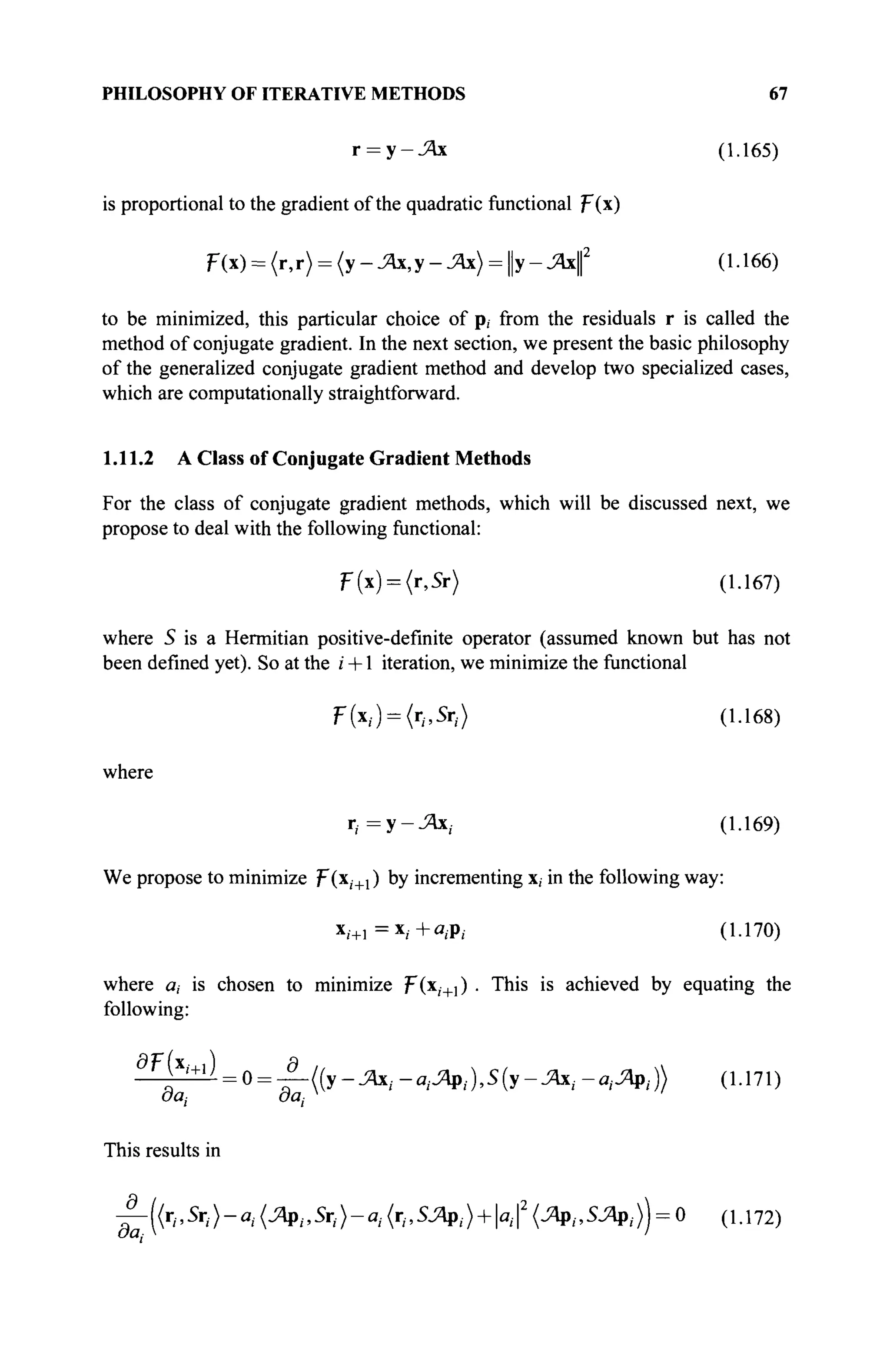
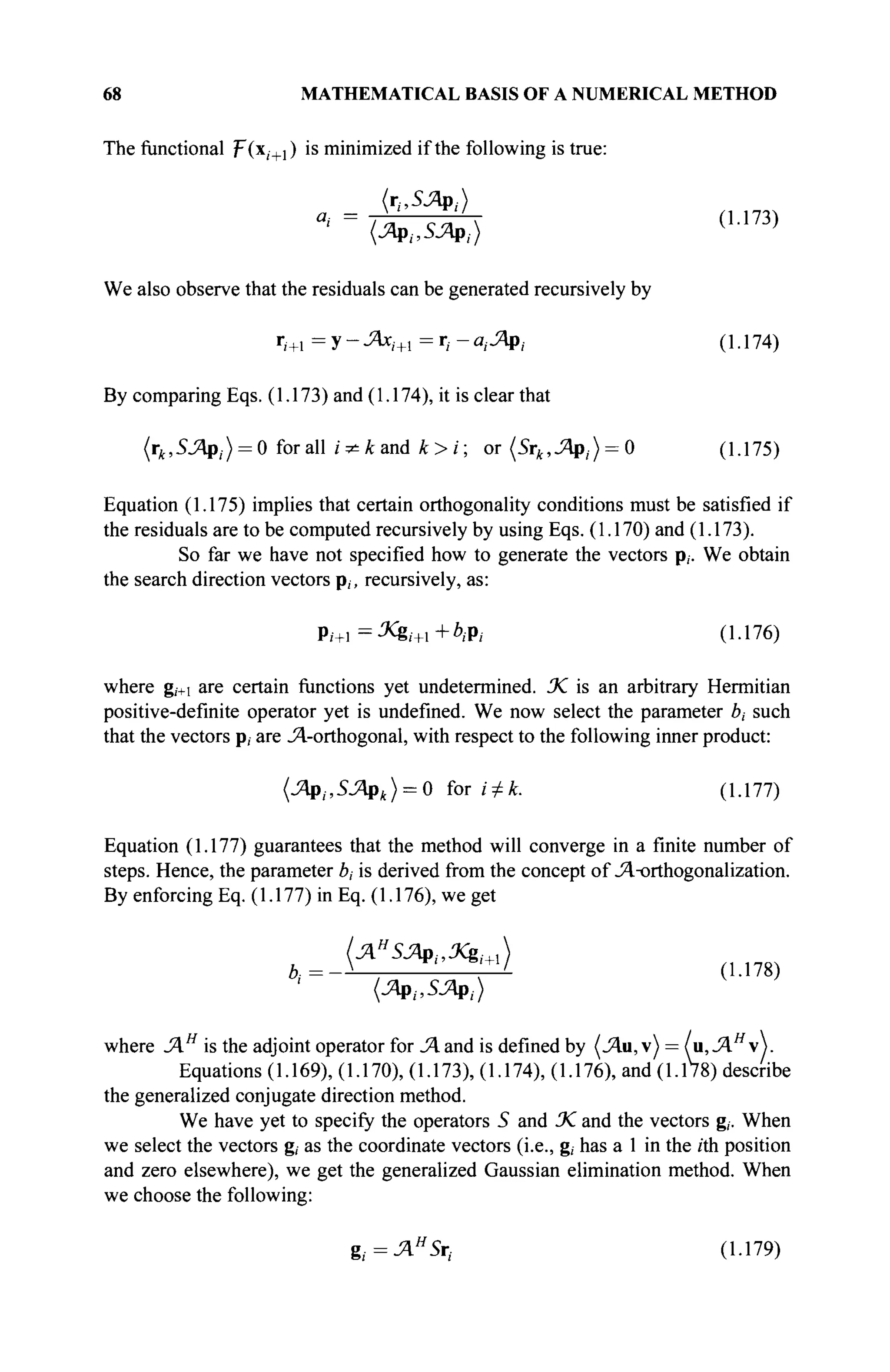
![PHILOSOPHY OF ITERATIVE METHODS 69
we get the class of conjugate gradient methods.
The conjugate gradient methods described in Eqs. (1.169), (1.170),
(1.173), (1.174), (1.176), and (1.179) all converge to the solution in a finite
number of steps starting with any initial guess [43-50].
We see that, for the class of conjugate gradient methods, the functional
F(x) is minimized at each iteration. Using the definition of the functional F(x)
of Eq. (1.168) we observe that it gets reduced at each iteration as
F(x/)-F(xi+,) = >0 (1.180)
In Eq. (1.180), the right-hand side of the equation is always positive, as 5 is a
positive definite operator, so that the error is minimized at each iteration and the
sequence x, converges.
Of course, it is well and good to know that the sequence x, converges, but
it is much better to know how it converges. If we introduce an operator T^such that
T = ΧΆΗ
ΞΛ (1.181)
and let
q = infinimum [spectrum (1)] = smallest eigenvalue of operator "T, when T b
a positive-definite matrix
Q = supremum [spectrum (T)] = largest eigenvalue of operator % when T^is a
positive-definite matrix
then it can be shown that the functional F(x) is minimized at each iteration and
that the rate of convergence at rth iteration is given by [43^45]
F(x,)<
2(1-a/
(l +Vä) '+(l->/ä) '
F(xo) (1.182)
and that the sequence of solutions x, converges to the exact solution x so that
i—v
1-Va
x, —x tends to zero faster than ._ where a = q/Q.ln the next section,
,1 + VaJ
we present two versions (special cases) of the conjugate gradient method. Each
special case has certain advantages. The reason we chose these two special cases is
because these two versions in particular lead to the simplest algorithm. We also
derive the rate of convergence of each of these techniques. Other special cases are
also possible, and they are presented elsewhere [51].](https://image.slidesharecdn.com/timeandfrequencydomainsolutionsofemproblemsusingintegralequationsandahybridmethodologyb-250205130750-568a5ba2/75/Time-and-Frequency-Domain-Solutions-of-EM-Problems-Using-Integral-Equations-and-a-Hybrid-Methodology-B-H-Jung-pdf-91-2048.jpg)
![70 MATHEMATICAL BASIS OF A NUMERICAL METHOD
1.11.2.1 Minimization of the Residuals (Conjugate Gradient Method A). For
this special case, we set
S = JC = I = Identity operator,
and so, from Eq. (1.181)
Τ = ΛΗ
Λ (1.183)
Also, one obtains
F(x,) = |h||2
(1.184)
The conjugate gradient method for this case starts with an initial guess x0 and
defines the following:
r0 =y-J2bc0 (1.185)
Р о = Л я
г 0 (1.186)
For / = 1,2,..., let:
P
a
i '-
X
/+l
r
i+i :
i+l =
b,=
11яя
г112
II ΊΙ
WM
= *ί+θ(Ρ/
= ri-aiJApi
AH
ri+]+biPi
II ΆΗ
Χ II2
II '+ΊΙ
|ля
г,.|2
(1.187)
(1.188)
(1.189)
(1.190)
(1.191)
By letting q and Q be the lower and upper spectral bounds for 'T = JAH
JA and by
setting a = q/Q, the characteristics of this method can be summarized as follows:
(1) The iterations described by Eqs. (1.185)—(1.191) is such that x, converges
to x for all initial guesses.
(2) ||r,|| is the least possible in / steps by using any iterative scheme of the
form Eq. (1.188).](https://image.slidesharecdn.com/timeandfrequencydomainsolutionsofemproblemsusingintegralequationsandahybridmethodologyb-250205130750-568a5ba2/75/Time-and-Frequency-Domain-Solutions-of-EM-Problems-Using-Integral-Equations-and-a-Hybrid-Methodology-B-H-Jung-pdf-92-2048.jpg)
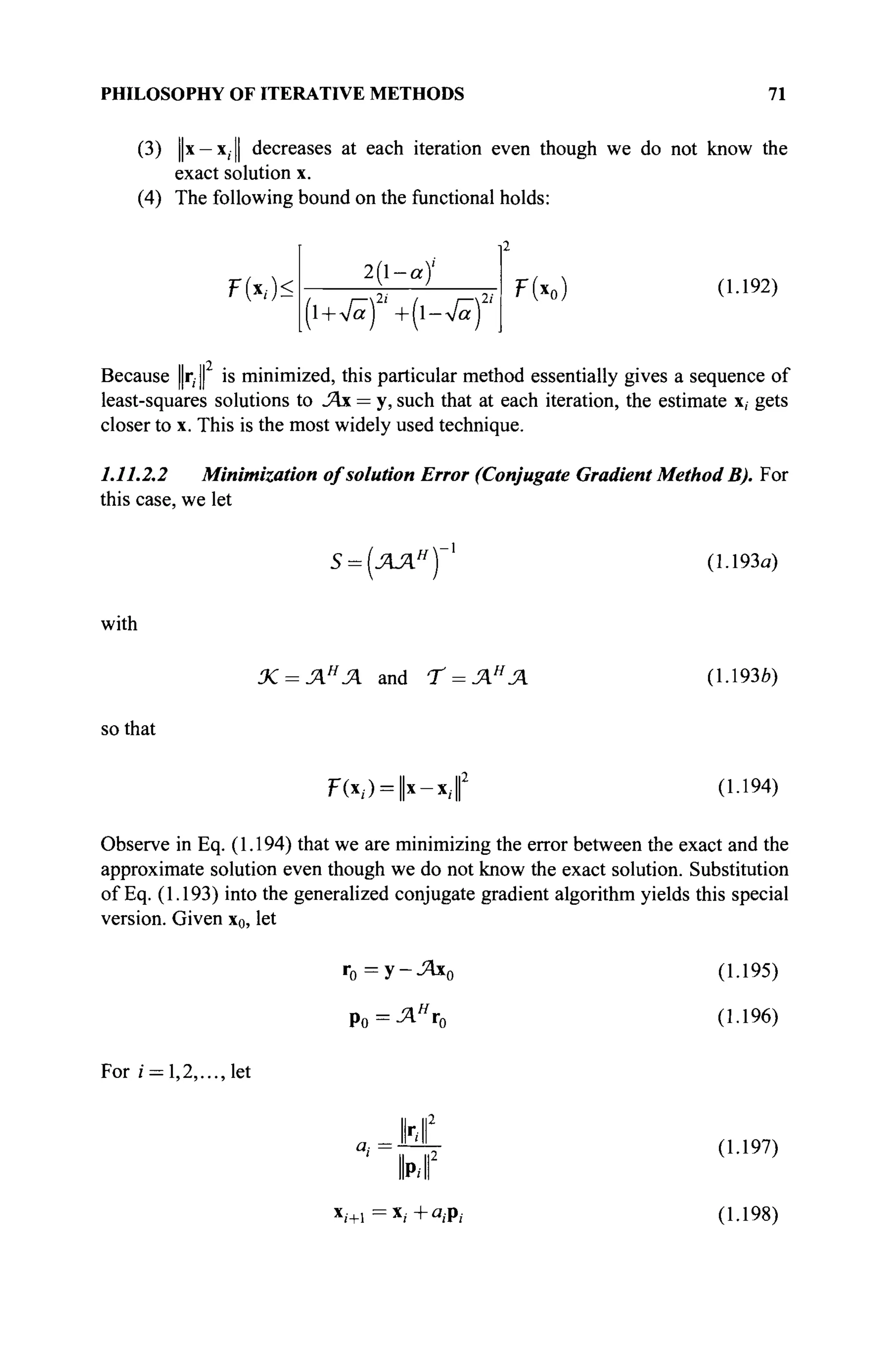
![72 MATHEMATICAL BASIS OF A NUMERICAL METHOD
1/+1=г
/-«.-ЯР/ (1-199)
р,.+ 1 =Лн
гж +6,.р; (1.200)
Il II2
b
'=Yf (L201)
By defining q and Q to be the lower and upper spectral bounds of 'T = Л Я
Л
and a = q/Q,we get the following results:
(1) The iteration is such that x, converges to x for all i.
(2) ||x — x; I is the least possible in i steps for all possible iterative methods of
the form Eq. (1.198) even though we do not know the exact solution.
(3) ||r,| may not decrease; in fact, at each iteration, it may even increase.
Often, it oscillates and does not get reduced until the last few iterations.
(4) The functional at each iteration is minimized, and the bound given by Eq.
(1.192) still holds.
Other special cases are available elsewhere [51].
Examples of the two iterative schemes and the type of results they generate
are discussed in the next section.
1.11.3 Numerical Examples
As an example, we consider the analysis of electromagnetic scattering from a 0.5λ
long antenna of radius 0.001λ, irradiated by a plane wave of amplitude 1 V/m. The
antenna is subdivided into 30 segments. Methods A and В are now applied directly
to the solution of the Pocklington's equation for the thin wire antenna [46]. So, in
this formulation, we bypass the matrix formulation stage. Both methods A and В
have been applied to solve the problem. The numerical computations obtained
from the two techniques are presented in Table 1.3.
Observe that, for method A, the magnitude of the residuals decrease
monotonically. For method B, even though the absolute error between the true
solution and the solution at the end of each iteration decrease, the residuals
actually increase and do not go down until the very end. Even though, from a
theoretical point of view, method В is attractive but from a numerical standpoint, it
seems both methods perform equally well. However, from a psychological point of
view, method A is preferred, as at each iteration, a user can observe the monotonie
convergence of the residuals as the iterative method progresses. The CPU time
taken by both techniques is almost the same. Observe both the methods even
converged into a good solution in 15 iterations, starting from a null initial guess.
The reason, these methods converged in 15 iterations is because the current
distribution on the structure is symmetrical about the midpoint of the antenna.](https://image.slidesharecdn.com/timeandfrequencydomainsolutionsofemproblemsusingintegralequationsandahybridmethodologyb-250205130750-568a5ba2/75/Time-and-Frequency-Domain-Solutions-of-EM-Problems-Using-Integral-Equations-and-a-Hybrid-Methodology-B-H-Jung-pdf-94-2048.jpg)
![PHILOSOPHY OF ITERATIVE METHODS 73
Hence, the operator would have two sets of eigenvalues that are equal. Because the
conjugate gradient method yields the solution in at most M steps, where M is the
number of independent eigenvalues of the operator (15 in this case), the method
converged in 15 iterations.
Table 1.3. Errors of the two versions of the conjugate gradient method (A and B)
Number of iterations Normalized error -
У
N
1
2
3
4
5
6
7
8
9
10
1
1
12
13
14
15
16
Method A
1.000
0.984
0.972
0.961
0.951
0.942
0.933
0.925
0.916
0.907
0.898
0.889
0.881
0.849
0.590
1.045 x 10⁴ 7
Method В
1.000
61.558
77.731
88.222
94.835
98.433
99.625
98.909
96.716
93.419
89.361
84.002
100.192
24.200
1.9308
1.013 x 10"
However, one disadvantage of the conjugate gradient method for a non-
self-adjoint operator is that, even though the method minimizes the quantity
Il H II2
ιι2
«Л rJ at each iteration, it does not guarantee that [|r( || , the residual is
minimized (i.e., how well the original equation Лх = у is satisfied). In fact, even
though ЛЯ
г, may be small at a particular iteration, ||r;|| could be very large.
Hence, the number of iterations taken by the iterative conjugate gradient method
|| ||2
for some problems can be large to minimize r,- to an acceptable level and,
therefore, can be less efficient than Gaussian elimination with pivoting. However,
when solving extremely large problems [52] in which one needs to have good
confidence on the final solution, it may be useful to follow the result obtained by
the Gaussian elimination with pivoting with a few steps of the conjugate gradient
method.](https://image.slidesharecdn.com/timeandfrequencydomainsolutionsofemproblemsusingintegralequationsandahybridmethodologyb-250205130750-568a5ba2/75/Time-and-Frequency-Domain-Solutions-of-EM-Problems-Using-Integral-Equations-and-a-Hybrid-Methodology-B-H-Jung-pdf-95-2048.jpg)
![74 MATHEMATICAL BASIS OF A NUMERICAL METHOD
1.12 THE DIFFERENCE BETWEEN APPLICATION OF THE
CONJUGATE GRADIENT METHOD (CGM) TO SOLVE A
MATRIX EQUATION AS OPPOSED TO DIRECT APPLICATION
OF CGM TO SOLUTION OF AN OPERATOR EQUATION
From the previous sections, it is clear that there are fundamental philosophical
differences between applying the conjugate gradient method to solve the moment
matrix equation of Eq. (1.113), as opposed to applying it to minimize Eq. (1.71)
recursively [50]. The difference is that the latter guarantees a strong convergence
of the residuals and the solution (depending on case A or case В [46]), whereas the
former guarantees weak convergence. The question now arises: Does this
difference still exist when we look at the problem from a computational point of
view? The answer is YES, and it is demonstrated by a simple example.
To illustrate this point, we start with an operator equation,
Я3 = у (1.202)
and through discretization for computational purposes, we convert it to a matrix
equation using the method of moment principles as
[Амрм} = Ы (1.203)
where [AM], [JM], and [YM] are the matrix version of the continuous operator
equation. If we now solve the matrix version in Eq. (1.203) by the conjugate
gradient method, then we are essentially solving the following equations, known
as the normal equations:
[Au]H
[AMpM} = [AM}H
[YM] (1.204)
where [AM]H
is the adjoint matrix of [AM] (which is simply the conjugate
transpose). Now, if we apply the conjugate gradient method directly to the solution
of the operator equation, then we solve
ΛΗ
Ά3 = ΆΗ
Υ (1.205)
Here JAH
is the adjoint operator. For numerical computation, Eq. (1.205) has to
be discretized to a matrix equation and we obtain
AH
D]AD]JD} = AZ[YD] (1.206)
It is seen that [AD] = [AM], [JD] = [JM], a n d
IY
D] = IY
MI Therefore, during
numerical implementation, the basic difference between Eqs. (1.204) and (1.206)
will be in how the continuous adjoint operator ΆΗ
has been discretized to [A" ]](https://image.slidesharecdn.com/timeandfrequencydomainsolutionsofemproblemsusingintegralequationsandahybridmethodologyb-250205130750-568a5ba2/75/Time-and-Frequency-Domain-Solutions-of-EM-Problems-Using-Integral-Equations-and-a-Hybrid-Methodology-B-H-Jung-pdf-96-2048.jpg)
![CONJUGATE GRADIENT APPLICATIONS 75
and whether the "matricized" adjoint operator [Ap ] is identical to the conjugate
transpose of the discretized original operator, [AM]H
. If the two matrices (namely
the discretized adjoint operator [A%] and the conjugate transpose of the
"matricized" operator [AM]H
)are not identical, then there will be a difference
between the applications of the conjugate gradient method to the solution of a
matrix equation, as opposed to the solution of the operator equation. For many
problems, Eqs. (1.204) and (1.206) are not identical.
For example, consider the convolution equation [3,50]
I x(t-u)v(u)du = y(t) for 0<f<oo (1.207)
where x(t) and y(t) are assumed to be known. We redefine Eq. (1.207) as
A = у . This operator equation can now be written in the matrix form, using the
method of moments concepts of pulse basis functions (piecewise-constant
functions) for the unknown v, and with impulse weighting, resulting in
[A/][VM] = [YM], or in a matrix form as
0
"•JV—1
0
0
X
N-M NxM
4
v2
V
M
=
Afxl
У
Уг
Уг
(1.208)
JVxl
If we now apply the conjugate gradient method to solve this matrix equation, we
will be solving [AMf[AM][VM]-.
case is
: [AMf[YM]. The adjoint matrix [AM]H
in this
Хл Х'у
0 je,
0 0
*JV-1
'■N-M
(1.209)
We get a solution for [V] (in this case) by solving Eq. (1.204) with the conjugate
gradient method. Now, let us apply the conjugate gradient method directly to the
operator equation as Eq. (1.207). We consider the adjoint operator for the integral
equation as Eq. (1.207). The adjoint operator, ΆΗ
, of JA, is defined by
(AV, Z) = (Y,AH
ZJ,OT equivalents, by
fz(t)dt fx(t-u)v(u)du = fv(u)du f z{t)x(t-u)dt (1.210)](https://image.slidesharecdn.com/timeandfrequencydomainsolutionsofemproblemsusingintegralequationsandahybridmethodologyb-250205130750-568a5ba2/75/Time-and-Frequency-Domain-Solutions-of-EM-Problems-Using-Integral-Equations-and-a-Hybrid-Methodology-B-H-Jung-pdf-97-2048.jpg)
![76 MATHEMATICAL BASIS OF A NUMERICAL METHOD
which is not a convolution but a correlation operation. We have observed in
section 1.6 that the adjoint of the convolution operator is the correlation operator,
which is similar to an advance convolution operator. By comparing Eqs. (1.209)
and (1.210), it is apparent that [AM]H
is a restricted version of the actual adjoint
operator in Eq. (1.210). This is because the adjoint operator is given by
ΛΗ
ζ= fz(t)x(t-u)dt (1-211)
This continuous operator can only take the form of under the assumption that
z(n) is identically zero beyond n, and this may not be true, in general. Therefore,
[Ap ] and [AM]H
are not identical for this problem unless some additional
assumptions are made! In the signal processing literature, a clear distinction has
been made between Eqs. (1.204) and (1.206). In Eq. (1.204), [AM]H
[AM] is
called the covariance matrix of the data, whereas [A%][AD] in Eq. (1.206) is
called the autocorrelation matrix of the data. It is well known that Eqs. (1.204) and
(1.206) yield different results. In the electromagnetics literature, several
techniques have been developed to solve Eq. (1.206). These techniques depend on
the assumptions that need to be made regarding the behavior of x and z for t > n .
One possible assumption may be that the waveforms become almost zero for
/ > n. An alternative numerical implementation has been considered in [53], in
which instead of assuming the nature of decay for x and z for t > n, a weighted
inner product has been defined to minimize the error introduced in discretizing the
continuous adjoint operator. However, for non-equally sampled data, no
generalization can be made.
Thus, it is important to note that the distinction between correlation
(1.211) and a convolution (1.207) disappears when the kernel is symmetric.
Therefore, in the frequency domain, a distinction between correlation and
convolution in an integral equation setting cannot be made as the Green's function
contains terms that are the absolute value of the distance and, therefore, is
symmetric. Hence, this distinction does not exist for problems defined in the
frequency domain. However, this is not true for time domain problems in which
the convolution operator is not similar to its adjoint, which is a correlation
operator as shown in [47].
1.13 CONCLUSION
This chapter begins by describing some fundamental mathematical definitions
related to the concepts of various spaces and defining the concept of convergence.
Next, the concept of an ill-posed and a well-posed problem is described
to illustrate that the concept of a solution to a problem may not be clearly defined.
Then an attempt has been made to bring out the mathematical differences
between the variational method (Rayleigh-Ritz), Galerkin's method, and the
method of least squares. It is seen that, for a variational method, the expansion](https://image.slidesharecdn.com/timeandfrequencydomainsolutionsofemproblemsusingintegralequationsandahybridmethodologyb-250205130750-568a5ba2/75/Time-and-Frequency-Domain-Solutions-of-EM-Problems-Using-Integral-Equations-and-a-Hybrid-Methodology-B-H-Jung-pdf-98-2048.jpg)
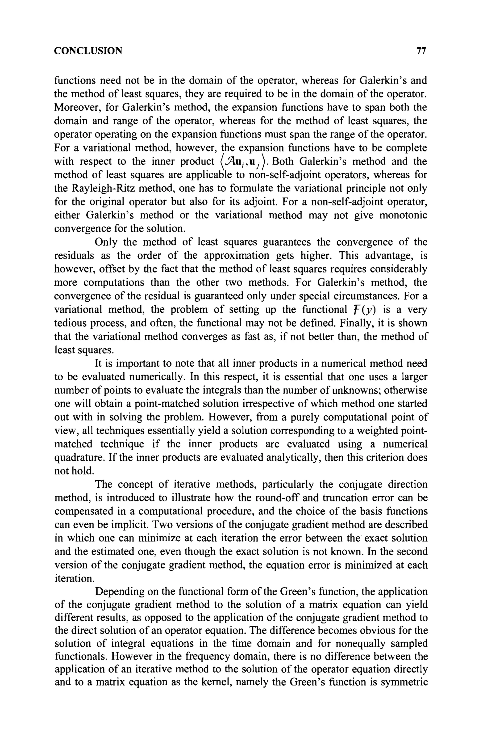
![78 MATHEMATICAL BASIS OF A NUMERICAL METHOD
in this case. However, because the kernel is not symmetric in the solution of a time
domain integral equation, the results will be different when an iterative method is
applied directly to the solution of an operator equation than applying it to the
solution of a matricized version of the operator equation because the adjoint of a
convolutional operator is the correlation operator.
REFERENCES
[I] F. Reza, Linear Spaces In Engineering, Ginn and Company, Waltham, Mass., 1971.
[2] R. F. Harrington, Methods of System Analysis, Lecture Notes, Department of
Electrical and Computer Engineering, Syracuse University, Syracuse, N.Y., 1971.
[3] I. Stakgold, Green's Functions and Boundary Value Problems, John Wiley & Sons,
New York, 1979.
[4] C. Dorny, A Vector Space Approach to Models and Optimization, John Wiley &
Sons, New York, 1975.
[5] T. K. Sarkar, D. D. Wiener, and V. K. Jain, "Some mathematical considerations in
dealing with the inverse problem," IEEE Trans. Antennas Prop., Mar. 1981, pp. 373-
379.
[6] M. Z. Nashed, "Approximate regularized solutions to improperly posed linear
integral and operator equations," in D. Colton and R. Gilbert, (eds.), Constructive and
Computational Methodsfor Differential and Integral Equations, Springer, New York,
1974, pp. 289-332.
[7] M. M. Lavrentiev, "Some improperly posed problems of mathematical physics," in
Tracts in Natural Philosophy, Vol. II., Springer-Verlag, Berlin, Germany, 1967.
[8] A. N. Tykhonov and V. Y. Arsenin, Solutions of Ill-Posed Problems, Wiley, New
York, 1997.
[9] D. L. Phillips, "A technique for the numerical solution of certain integral equations of
the first kind," J. Assoc. Comput. Mach., Vol. 9, pp. 84-97, 1962.
[10] S. Twomey, "On numerical solution of Fredholm integral equations of the first kind
by the inversion of the linear system produced by quadrature," J. Assoc. Comput.
Mach., Vol. 10, pp. 97-101, 1963.
[II] S. Twomey, "The application of numerical filtering to the solution of integral
equations encountered in indirect sensing measurements," J. Franklin Inst., pp. 95-
109, 1965.
[12] W. L. Perry, "Approximate solution of inverse problems with piecewise continuous
solutions," Radio Sei., Vol. 12, pp. 637-642, 1977.
[13] A. E. Hoerl and R. W. Kennard, "Ridge regression—Past, present, and future," Int.
Symp. Ill-Posed Problems: Theory and Practice, University of Delaware, Newark,
Oct. 1979.
[14] M. Z. Nashed, Ed., Generalized Inverses and Applications, Academic, New York,
1976.
[15] R. M. Lewis, "Physical optics inverse diffraction," IEEE Trans. Antennas Prop., Vol.
AP-17,pp. 308-314, 1969.
[16] N. N. Bojarski, Three-Dimensional Electromagnetic Short Pulse Inverse Scattering,
Syracuse University Res. Corp., Syracuse, N.Y., 1967.
[17] W. L. Perry, "On the Bojarski-Lewis inverse scattering method," IEEE Trans.
Antennas Prop., Vol. AP-22, pp. 826-829, 1974.
[18] V. F. Turchin, V. P. Kozlov, and M. S. Malkevich, "The use of mathematical
statistics methods in the solution of incorrectly posed problems," Soviet Phys.
Uspekhi, Vol. 13, pp. 681-703, 1971.](https://image.slidesharecdn.com/timeandfrequencydomainsolutionsofemproblemsusingintegralequationsandahybridmethodologyb-250205130750-568a5ba2/75/Time-and-Frequency-Domain-Solutions-of-EM-Problems-Using-Integral-Equations-and-a-Hybrid-Methodology-B-H-Jung-pdf-100-2048.jpg)
![80 MATHEMATICAL BASIS OF A NUMERICAL METHOD
[43] M. K. Hestenes, "Applications of the theory of quadratic forms in Hubert space in the
calculus of variations," Pacific J. Math., Vol. 1, pp. 525-581, 1951.
[44] K. M. Hayes, "Iterative methods for solving linear problems in Hubert space," in O.
Taussky (ed.), Contributions to Solution of Systems of Linear Equations and
Determination of Eigenvalues, Vol. 39, Nat. Bur. Standards, Appl. Math., 1954, pp.
71-104.
[45] M. K. Hestenes and B. Steifel, "Method of conjugate gradients for solving linear
systems," J. Res. Nat. Bur. Standards, Vol. 49, pp. 409-436, 1952.
[46] T. K. Sarkar, "The application of the conjugate gradient method for the solution of
operator equations arising in electromagnetic scattering from wire antennas," Radio
SW.,Vol. 19, pp. 1156-1172, 1984.
[47] T. K. Sarkar, S. M. Rao, and S. A. Dianat, "The application of the conjugate gradient
method to the solution of transient electromagnetic scattering from thin wires," Radio
S«., Vol. 19, pp. 1319-1326, 1984.
[48] T. K. Sarkar and E. Arvas, "On a class of finite step iterative methods (conjugate
directions) for the solution of an operator equation arising in electromagnetics," IEEE
Trans. Antennas Prop., Vol. 33, pp. 1058-1066, 1985.
[49] T. K. Sarkar, E. Arvas, and S. M. Rao, "Application of FFT and the Conjugate
Gradient Method for the Solution of Electromagnetic Radiation from Electrically
Large and Small Conducting Bodies," IEEE Transactions on Antennas and
Propagation, Vol. 34, No. 5, pp. 635-640, May 1986.
[50] T. K. Sarkar (ed.), Application of the Conjugate Gradient Method in
Electromagnetics and Signal Processing, Elsevier, New York, 1991.
[51] M. Hestenes, Conjugate Direction Methods in Optimization, Springer Verlag, Berlin,
Germany, 1978.
[52] Y. Zhang and T. K. Sarkar, Parallel Solution of Integral Equation-Based EM
Problems in the Frequency Domain, John Wiley & Sons, Hoboken, N.J., 2009.
[53] F. I. Tseng and T. K. Sarkar, "Deconvolution of the impulse response of a conducting
sphere by the conjugate gradient method," IEEE Trans. Antennas Prop., Vol. 35, pp.
105-110,1987.](https://image.slidesharecdn.com/timeandfrequencydomainsolutionsofemproblemsusingintegralequationsandahybridmethodologyb-250205130750-568a5ba2/75/Time-and-Frequency-Domain-Solutions-of-EM-Problems-Using-Integral-Equations-and-a-Hybrid-Methodology-B-H-Jung-pdf-102-2048.jpg)
![2
ANALYSIS OF CONDUCTING
STRUCTURES IN THE FREQUENCY
DOMAIN
2.0 SUMMARY
In this chapter, the numerical procedures for analyzing the electromagnetic
scattering from an arbitrarily-shaped conducting object in the frequency domain
are presented. Based on the boundary condition of the electric or the magnetic
fields, two different integral equations for analyzing the scattering problems for
conducting objects are derived and termed as the electric field integral equation
(EFIE) and the magnetic field integral equation (MFIE). In addition, these two
integral equations can be combined to form a more general formulation called the
combined field integral equation (CFIE). The EFIE can be used for objects with
both closed and open surfaces, whereas the MFIE and CFIE are suitable only for
closed structures. All these equations can be represented as a function of the
induced surface current density. The scattered field can be calculated using the
current density obtained by solving one of these equations. The integral equations
(i.e., EFIE, MFIE, and CFIE), can be solved numerically using the method of
moments through the triangular patch modeling scheme using the well-known
triangular patch or the Rao-Wilton-Glisson (RWG) basis functions. Once the
current distribution on the structure is obtained, the fields scattered from the
structure of interest can be evaluated.
2.1 INTRODUCTION
Research in electromagnetics (EM) has been pursued at a fast pace. The major
efforts have been placed in the development of the general purpose computational
methodology, yielding a good enough approximation for the exact solution. An
important breakthrough is that the solution to the intricate EM formulations can be
obtained more efficiently by taking full advantage of the fast digital computers
available today. The evolution of computer hardware and software further enables
the electromagnetic analysis for large or complicated targets to be completed in an
acceptable amount of time [1]. Analyzing electromagnetic radiation and scattering
81
Time and Frequency Domain Solutions of EM Problems
Using Integral Equations and a Hybrid Methodology
by B. H. Jung, T. K. Sarkar, S. W. Ting, Y. Zhang, Z. Mei, Z. Ji,
M. Yuan, A. De, M. Salazar-Palma, and S. M. Rao
Copyright © 2010 John Wiley & Sons, Inc.](https://image.slidesharecdn.com/timeandfrequencydomainsolutionsofemproblemsusingintegralequationsandahybridmethodologyb-250205130750-568a5ba2/75/Time-and-Frequency-Domain-Solutions-of-EM-Problems-Using-Integral-Equations-and-a-Hybrid-Methodology-B-H-Jung-pdf-103-2048.jpg)
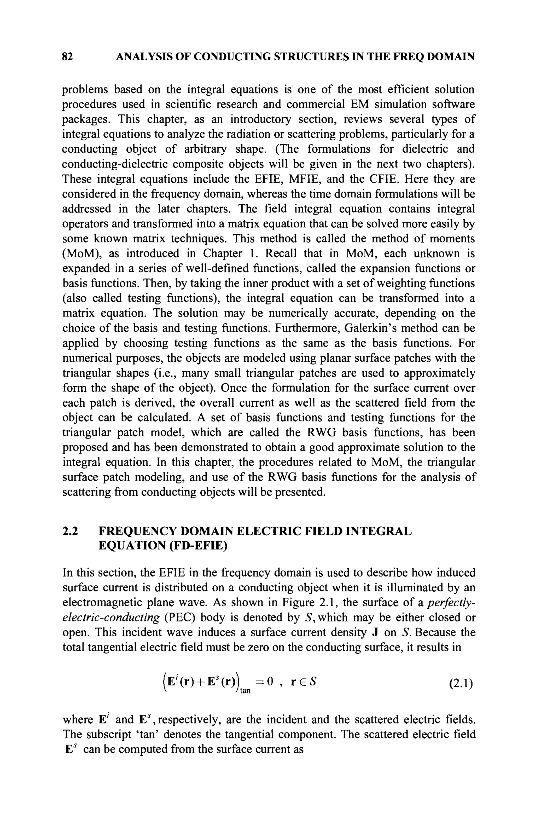
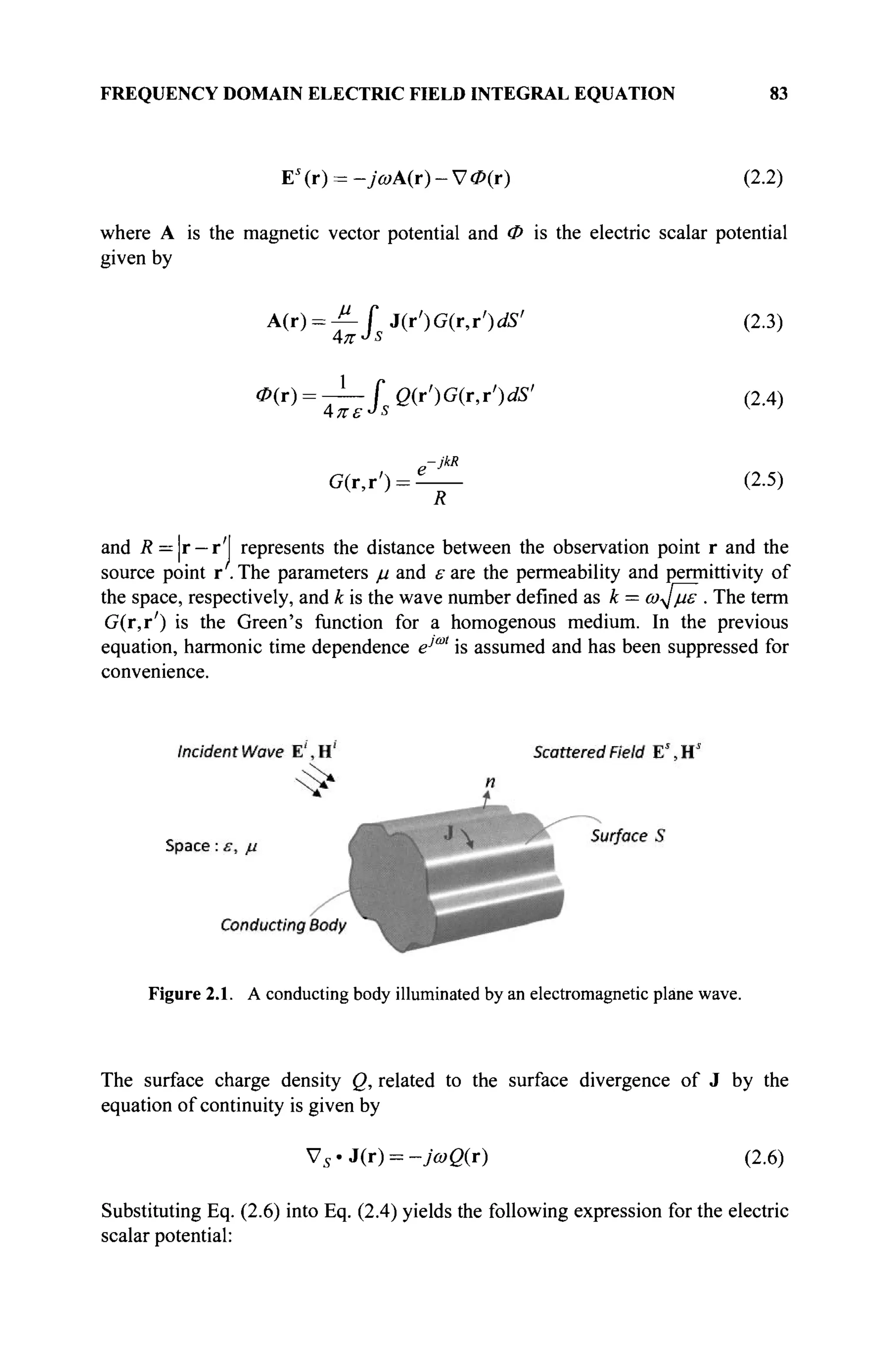
![84 ANALYSIS OF CONDUCTING STRUCTURES IN THE FREQ DOMAIN
0(T) = -^—fVs-J(T')G(r,r')dS' (2.7)
Then, substituting Eq. (2.2) into Eq. (2.1) and grouped with Eqs. (2.3) and (2.7),
the relation in the frequency domain can be obtained between the incident electric
field and the induced surface current density. It is generally known as the
frequency domain EFIE.
(>A(r) + V*(r))t B n =(Ei
(r))t o (2.8«)
A
^ = T~ U(r')G(r,r')dS' (2.8b)
0{t) = -J— fv'S'3(jr')G(r,r')dS' (2.8c)
where r e S. This EFIE cannot be solved exactly using analytical methods only
and thus a numerical solution is often used instead. One accurate and efficient
method to numerically solve the unknown surface current in the previous EFIE is
to apply the MoM along with the triangular surface patch model and the RWG
basis functions. The basic concept of MoM, which has been given in Chapter 1, is
to convert an operator equation into a matrix equation using a set of basis and
testing functions. To determine the current, the surface of the object is usually
modeled by the combination of many small triangular patches. The calculation
will be carried out patch by patch, and the overall surface current can be obtained
by summing up the contributions over all the patches. The accuracy of the MoM is
indeed dependent on the selection of basis and testing functions. One common
choice is the RWG function. The detailed procedures of the numerical method will
be presented in the following sections.
2.3 TRIANGULAR SURFACE PATCH MODELING
To model an arbitrarily shaped surface, planar triangular patch modeling is
particularly appropriate, as it is can accurately conform to any geometrical surface
or boundary [2]. This patching scheme is easily specified as a possible computer
input; a varying patch density can be used according to the resolution required in
the surface geometry or induced current, and mathematically simple basis
functions can be defined with no bothersome line charges along the boundary.
Detailed considerations for patch modeling of arbitrary surfaces may be seen in [3].
Assuming that the structure to be studied is approximated by many planar
triangular patches, consider a pair of triangles Γ„+
and T~ connected with the nth
nonboundary edge, as illustrated in Figure 2.2.](https://image.slidesharecdn.com/timeandfrequencydomainsolutionsofemproblemsusingintegralequationsandahybridmethodologyb-250205130750-568a5ba2/75/Time-and-Frequency-Domain-Solutions-of-EM-Problems-Using-Integral-Equations-and-a-Hybrid-Methodology-B-H-Jung-pdf-106-2048.jpg)
![TRIANGULAR SURFACE PATCH MODELING 85
Figure 2.2. A pair of triangular patches associated with a nonboundary edge.
In Figure 2.2, /„ is the length of the nonboundary edge (edge common to both
triangles) and a^ and a~ are the areas of the triangles Γη
+
and T~, respectively.
Vectors p+ and p~ are the position vectors defined with respect to the free
vertices (vertices not connected to the common edge) of Γ„+
and T~ , respectively.
The position vector pjj" is oriented from the free vertex of Гя
+
to any point inside
the triangle. Similar remarks can be applied to the position vector p~, except its
direction is toward the free vertex from any point in T~. The plus or minus
designation of the triangles is defined based on the assumption that the positive
direction of the current flowing is from the triangle Г„+
to T~ . From the
properties of the RWG basis [2], the expansion function associated with the «th
edge is defined on the pair of adjacent triangular patches as
f„(r) = f„+
(r) + f„-(r)
^(••l·
- ^ - p ±
, г е Г е
О, г^Г±
(2.9a)
(2.9b)
Then the surface divergence of this basis function can be calculated [2] using
a/ ±f
(zbl/p^ I —-—;—-, which results in
1 j
d9n
Vs -f„(r) = V5.f„+
(r) + V5.f„-(r) (2.10a)
Vs'tfir):
0, x<jLT± (2.106)](https://image.slidesharecdn.com/timeandfrequencydomainsolutionsofemproblemsusingintegralequationsandahybridmethodologyb-250205130750-568a5ba2/75/Time-and-Frequency-Domain-Solutions-of-EM-Problems-Using-Integral-Equations-and-a-Hybrid-Methodology-B-H-Jung-pdf-107-2048.jpg)
![86 ANALYSIS OF CONDUCTING STRUCTURES IN THE FREQ DOMAIN
With the defined expansion function, the solution of the EFIE can be found by the
MoM.
2.4 SOLUTION OF THE EFIE
As has been introduced in Chapter 1, a general operator equation given by
-Cx = y (2.11)
can be solved by using the method of moment. In this section, the MoM steps are
outlined to provide a more complete description of this solution procedure. The
MoM starts with using a set of expansion functions or basis functions f„ to
represent the unknown
N
x=X>,f, (2.12)
/=1
The operator equation in Eq. (2.11) is then expressed by
£х = Х>,.Д.=у (2.13)
i=l
To weigh the approximation error to zero with respect to a certain set of weighting
functions or testing functions Wy,the inner product of Eq. (2.13) with W· results
in
J2a
i(£f
i>W
j) = (y>W
j) for j = l,2,...,N (2.14)
!=1
This set of equations can be represented in a matrix form as
Ы Ы = Ы (2-15)
In Eq. (2.15), [a] is the unknown to be solved for a given [y] and, thus, leads to
the solution of the original operator equation in Eq. (2.11). In the testing
procedure, the complex inner products are used. Some important properties of the
inner product are listed in section 1.3.5. From Eq. (1.9), the inner product for two
vector functions f and g is defined as
M = fsi-gdS (2.16)](https://image.slidesharecdn.com/timeandfrequencydomainsolutionsofemproblemsusingintegralequationsandahybridmethodologyb-250205130750-568a5ba2/75/Time-and-Frequency-Domain-Solutions-of-EM-Problems-Using-Integral-Equations-and-a-Hybrid-Methodology-B-H-Jung-pdf-108-2048.jpg)
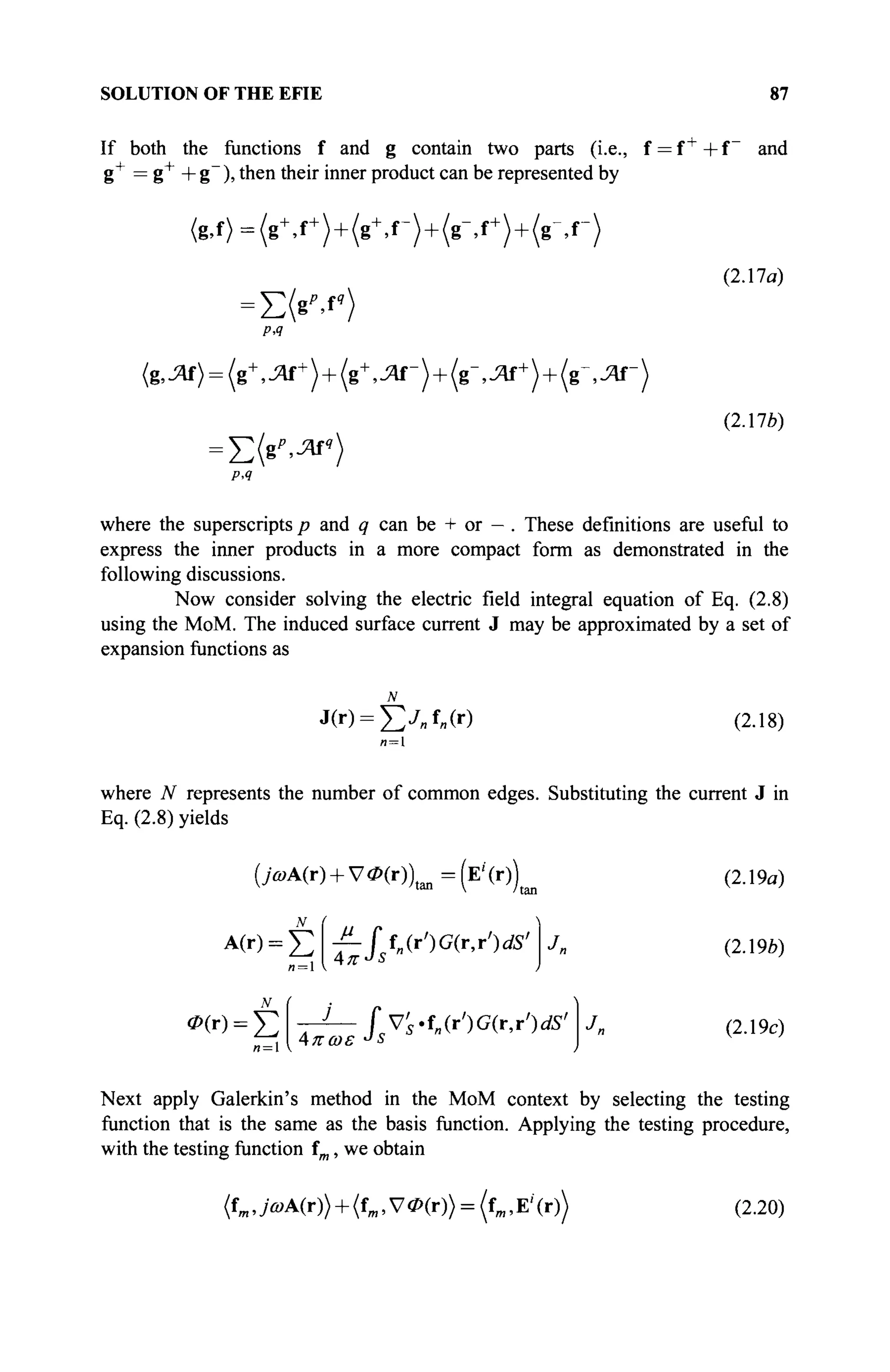
![88 ANALYSIS OF CONDUCTING STRUCTURES IN THE FREQ DOMAIN
for m = 1, 2,..., N. The first term in Eq. (2.20) becomes
(fm ,>A(r)) = £ i£Ulftm(r)./ f„(r') G(r.r') dS' dS (2.21)
or equivalently
(fm, 7®A(r)) = y© / / £ Лт„ J„
л = 1
4™ = 7 " / * Л ( г )
' f' f„(r')G(r,r') dS'dS
Ц-7Г *J Ъ *J О
(2.22α)
(2.22e)
The second term in Eq. (2.20) contains the testing of the gradient of the electric
scalar potential. This task can be accomplished by using the vector identity
ν · ( Μ ) = Α·(ν^) + ^(ν·Α) or Α·(ν^) = ν·(φΑ)-φ(ν·Α).
(fm,S70(r)) = fsVs-{fm0(r)) dS-fs(Vs'fm) <P(r) dS (2.23)
The first term in Eq. (2.23) can be converted into a contour integral using the
Stoke's theorem. Because the normal component of the basis function is zero
along the contour [3], we have
/J V5 .(f„I <P(r))dS = 0 (2.24)
Therefore, the second term in Eq. (2.20) can be written as
(fm,V0(r)) = -fs(Vs· fm) <P(r) dS (2.25)
Now substitute the scalar potential Φ given by Eq. (2.19c) into Eq. (2.25)
(fm,V0(r)) = - £ ^ - / s V s . f m ( r ) J V s · f„(r')G(r,rVS'dS Jn (2.26)
resulting in
{fm,V0(r)) = -^L-f2BmnJn
ωε
(2.27a)
n = l](https://image.slidesharecdn.com/timeandfrequencydomainsolutionsofemproblemsusingintegralequationsandahybridmethodologyb-250205130750-568a5ba2/75/Time-and-Frequency-Domain-Solutions-of-EM-Problems-Using-Integral-Equations-and-a-Hybrid-Methodology-B-H-Jung-pdf-110-2048.jpg)
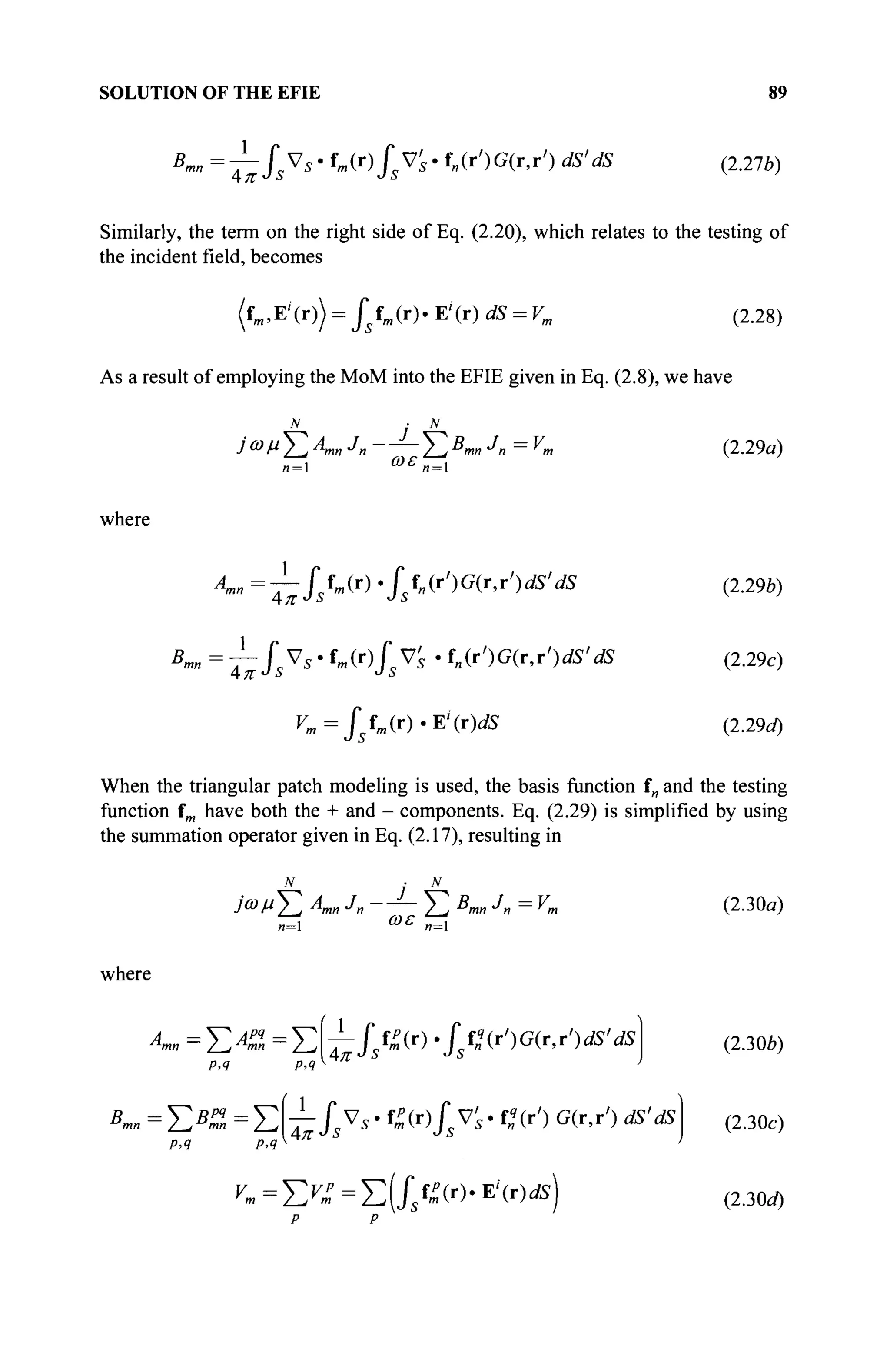
![90 ANALYSIS OF CONDUCTING STRUCTURES IN THE FREQ DOMAIN
Substituting the basis and testing functions on the triangular patches defined in Eq.
(2.9b) and their divergence given by Eq. (2.106) into Eq. (2.30) and approximating
the average charge density by the value of p at the centroid of the triangular patch
and, in addition, approximating the distance by r^ is equivalent to replacing the
integral over the testing triangle by its value at the centroid as seen in Figure 2.3
[2]. In addition, one obtains
(a:+a-)tr^ J t„dS = ^ ( Ρ Γ + Ρ Γ ) = ' « ( Γ Γ - Ι Γ )
resulting in
J1- | J-
(2.3 la)
Ja>vT^AmnJn-
n= ωε
/ ; "mn J
n ~ * m
n=l
(2.3 le)
where
A = S^ Apq
= V
mn / j mn / j
Ρ·4
и,
6π
mj_n_ cp %
rm -f 9"
«JTSVn
-JkRP
В =V5P
'=±V
P,4 P,4
4
а^тГ" RP
jkRg
dS'
IlL±r ^ _
π aï Jrg Ri
dS'
(2.3 le)
(2.3 d)
^=Σ^=Στρ
»'Ε
'(Γ
^)
p P
(2.3 le)
and RP =|r
mP — Γ
Ί· The sign in Eq. (2.3 la) is positive, when p and q are the
same and negative otherwise.
Figure 2.3. Centroid approximations on the triangular patches.](https://image.slidesharecdn.com/timeandfrequencydomainsolutionsofemproblemsusingintegralequationsandahybridmethodologyb-250205130750-568a5ba2/75/Time-and-Frequency-Domain-Solutions-of-EM-Problems-Using-Integral-Equations-and-a-Hybrid-Methodology-B-H-Jung-pdf-112-2048.jpg)
![FREQUENCY DOMAIN MAGNETIC FIELD INTEGRAL EQUATION 91
The integrals in Eqs. (2.31c) and (2.3Id) may be evaluated by the method
described in [4]. Furthermore, Eq. (2.316) can be expressed as
Σ Z
mn Jn = v
m (2.32)
where
я = 1
Zmn = ΐωμΑ^, —J
—Bmn = jfy
ωε
D
A mn
(2.33)
In Eq. (2.33), the parameter к is the wave number and parameter η is the intrinsic
wave impedance defined as η = ^μΙ ε. Equation (2.32) is associated with each
common edge, for m = l,2,...,N, and it finally may be written in a matrix form
as
[Zmn][J
n = K (2.34)
where [Zmn] is a NxN matrix and [Jn] and [Vm] are column vectors of length
N. The solution of Eq. (2.34) is a column vector of the coefficients of current
expansion [./„], and thus, it can lead to the solution of current density as well as
the scattered electric field.
2.5 FREQUENCY DOMAIN MAGNETIC FIELD INTEGRAL
EQUATION (FD-MFIE)
Applying the boundary condition for the magnetic field, a MFIE for a closed
conducting body may be derived as follows. Let S represent the surface of a
closed conducting body that is illuminated by an electromagnetic wave. Also, let
H' represent the incident magnetic field and Hs
represent the scattered magnetic
field caused by the induced current J. Then we have,
n x (Нг
' (r) + HJ
(r)) = J(r), r e S (2.35)
where n represents an outward-directed unit vector normal to the surface S at a
field point r. Note that the body must be a closed body to define a unique outward
normal vector. The scattered field can be written in terms of the magnetic vector
potential function, given by
Н » = - У х А ( г ) (2.36)](https://image.slidesharecdn.com/timeandfrequencydomainsolutionsofemproblemsusingintegralequationsandahybridmethodologyb-250205130750-568a5ba2/75/Time-and-Frequency-Domain-Solutions-of-EM-Problems-Using-Integral-Equations-and-a-Hybrid-Methodology-B-H-Jung-pdf-113-2048.jpg)
![92 ANALYSIS OF CONDUCTING STRUCTURES IN THE FREQ DOMAIN
It is noted that the magnetic vector potential A is the same as in Eq. (2.3).
Applying the Cauchy principal value to the curl term, Eq. (2.36) can be rewritten
as [5]
nxHs
(r) = - ^ + n x - V x À ( r ) (2.37)
2 μ
where
Ä
W = ΊΓ L J(r')G(r,r')«œ' (2.38)
In Eq. (2.38), S0 denotes the surface with the removal of the singularity at r = r'
(or R = 0 ) from the surface S. Note that Eq. (2.35) along with Eq. (2.37)
represents the magnetic field integral equation. Now substituting Eq. (2.37) into
Eq. (2.35), we obtain the relation between the incident magnetic field and the
induced surface current density, and it is generally called the frequency domain
MFIE. It is given by
- ^ - n x - V x Ä ( r ) = nxH'(r) (2.39)
2 μ
2.6 SOLUTION OF THE MFIE
Employing the testing procedure of the MoM to Eq. (2.39) results in the matrix
equation
J(r) / , 1
'm'
tm, n x - V x Â(r) = (fm, n x H'' (r)) (2.40)
2 1 m '
I t*
The surface current is approximated by the current expansion functions,
J(r) = £yBfe(r)
л = 1
as described in Eq. (2.9). The first term of the inner product in Eq. (2.40) yields
f
m
'Щ=
έ 1/л(г)
·f
«(r) ds
)j
- <2
·41
)
or equivalently
ff^^WE^·7
« (2.42a)
n =](https://image.slidesharecdn.com/timeandfrequencydomainsolutionsofemproblemsusingintegralequationsandahybridmethodologyb-250205130750-568a5ba2/75/Time-and-Frequency-Domain-Solutions-of-EM-Problems-Using-Integral-Equations-and-a-Hybrid-Methodology-B-H-Jung-pdf-114-2048.jpg)
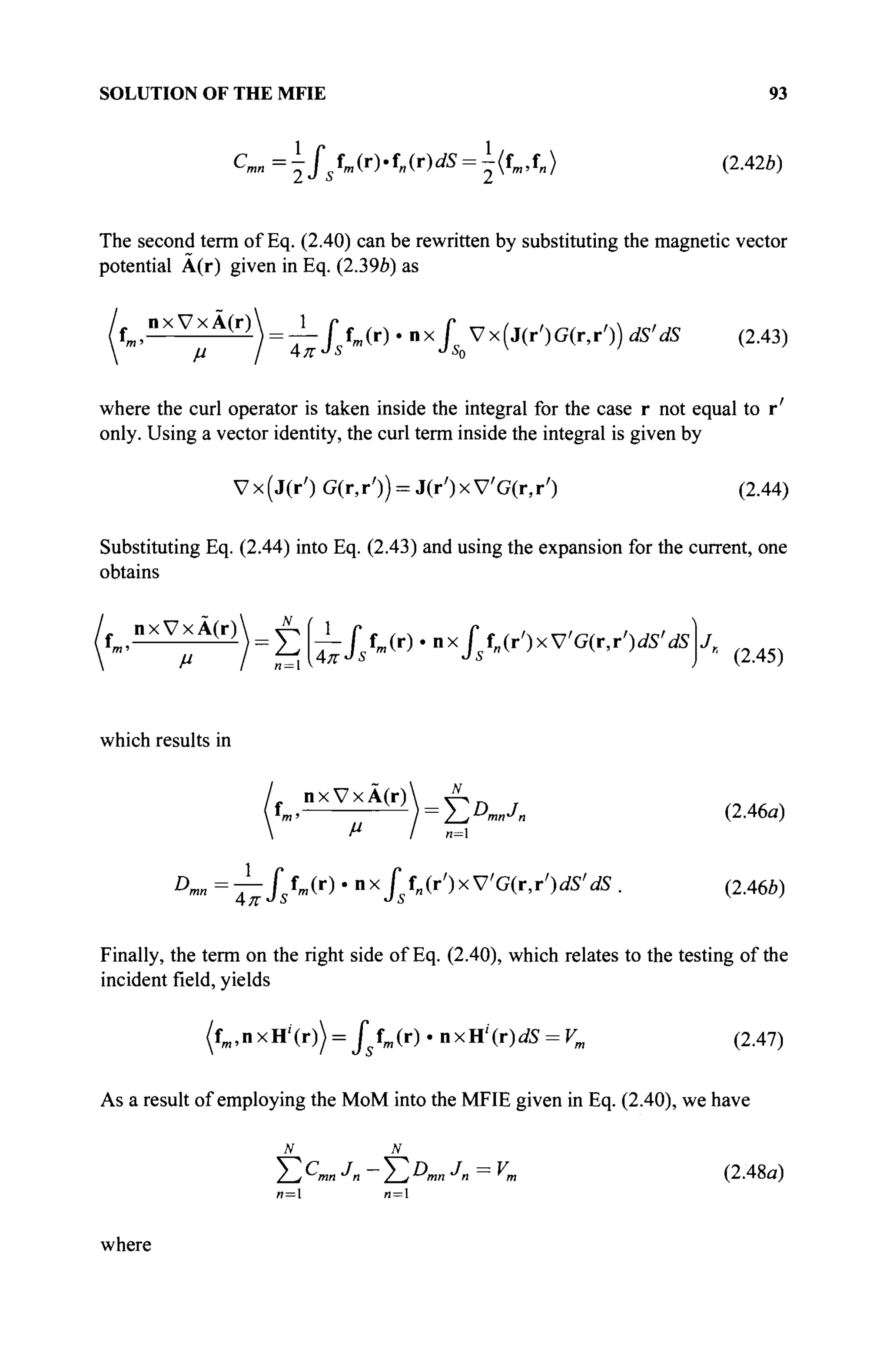
![94 ANALYSIS OF CONDUCTING STRUCTURES IN THE FREQ DOMAIN
Cmn = J fm(r)'fn(r)dS = Utm,t„)
Dmn = — Г fm(r).nx Г f„(r')xV'G(r,rVS'
Д. IT *J à *J Л
dS
^ = / Μ Γ ) . Ι Ι Χ Η ' ( Γ ) dS
(2.48b)
(2.48c)
(2.48c/)
When the RWG modeling is used, the basis function f„ and testing function fm
have both + and - components. Thus, Eq. (2.48) results in
2^i mn^n 2-J m" " ~~ m
n= n=
where
cm„=Ec
^=E vkffi-n*
p,q р<я
Dmn = E D
™ = Σ T - / / » ( r )
' n x
/ / " ( r
' ) x V
' G ( r
' r
' ) i f f i
'
p,q p,q π
dS
^=Σ^=Σ(//^(Γ
)·ηχΗί
(Γ
) dS
(2.49a)
(2.49b)
(2.49c)
(2.49û0
Substituting the basis and testing functions on the triangular patches in Eq. (2.9Z>)
into Eq. (2.49) and approximating the average charge density by the value of p at
the centroid of the triangular patch, and in addition approximating the distance by
r^f, one obtains using the procedure described in [2]
/__,У-Ίηη J» / jmn J n ~ "m
n = n =
where
ppq I m ^η
8α?
3 I rn2
1 /l |2 i |2 i |2
4i m
I i ? v m l
l Im 2
l I m 3
i
~r
m ( r
m l + r
« l ) + r
mlr
nl
jkR
Dpq — U n [ pP.nx f plxR( + jkR)^r-dS'dS
V£=fp%-nxH'(rZ)
(2.50a)
(2.50b)
(2.50c)
(2.50d)](https://image.slidesharecdn.com/timeandfrequencydomainsolutionsofemproblemsusingintegralequationsandahybridmethodologyb-250205130750-568a5ba2/75/Time-and-Frequency-Domain-Solutions-of-EM-Problems-Using-Integral-Equations-and-a-Hybrid-Methodology-B-H-Jung-pdf-116-2048.jpg)
![FREQUENCY DOMAIN COMBINED FIELD INTEGRAL EQUATION 95
where rml, rm2, and rm3 are the position vectors from the three vertices of the
triangle T%, and r^ is the centroid of triangle τ£. rml and rnl are position
vectors of the free vertex of triangle τ£ and Tfj, respectively. Note that if the field
point does not lie on the triangle T^ (i.e., r^Tn
9
)the result is C^n =0. In Eq.
(2.49), the sign is positive when p and q are the same and is negative otherwise.
The expression in Eq. (2.506) is zero if m and n do not share a common triangle,
and it is twice the value if m = п. The integral in Eq. (2.50c) may be computed
numerically using the Gaussian quadrature. In Eq. (2.50tf*), n is associated with the
source triangle. Furthermore, Eq. (2.50a) can be expressed as
N
T,ZmnJn=Vm (2.51)
/1 = 1
where
^mn =
^ш —
^mn (2-52)
Equation (2.51) is associated with each common edge, for m = ,2,...,N.
Finally, it may be written in a matrix form as
[Zmn}{J„} = K] (2.53)
where [Zmn] is a NxN matrix and [Jn] and [Vm] are column vectors of length
N. The solution of Eq. (2.53) is a column vector of the coefficients of the current
expansion[J„], and thus, it can provide a solution to the current density and leads
to the analysis of the scattered field. Comparing Eq. (2.53) with Eq. (2.34), it is
noted that both the MFIE and EFIE have a similar form.
2.7 FREQUENCY DOMAIN COMBINED FIELD INTEGRAL
EQUATION (FD-CFIE)
In the analysis of closed conducting bodies at the frequencies corresponding to the
internal resonance of the structure, spurious solutions may be produced when
either the EFIE or MFIE is used. This is because the operator is singular at an
internal resonant frequency of the closed structure. One possible way to obtain a
unique solution for closed bodies at this internal resonant frequency is to combine
the EFIE and MFIE in a linear fashion. This combination results in the CFIE. The
frequency domain CFIE is obtained by a linear combination of the EFIE with the
MFIE [5] through
(1-*г)(-Е'(г)) +Ki7(j(r)-nxH'(r))
= ( l - f f ) ( E ' ( r ) | t m + ^ ( n x H i
( r ) ) (2.54)](https://image.slidesharecdn.com/timeandfrequencydomainsolutionsofemproblemsusingintegralequationsandahybridmethodologyb-250205130750-568a5ba2/75/Time-and-Frequency-Domain-Solutions-of-EM-Problems-Using-Integral-Equations-and-a-Hybrid-Methodology-B-H-Jung-pdf-117-2048.jpg)
![96 ANALYSIS OF CONDUCTING STRUCTURES IN THE FREQ DOMAIN
where
where к is the parameter of linear combination, which is between 0 (EFIE) and 1
(MFIE), and η is the wave impedance of the space.
The matrix equations of EFIE and MFIE, which are given by Eq. (2.34)
and Eq. (2.53), respectively, can be rewritten as
~ZE
mnJn) = [v* (2.55)
Z%n[Jn = [v% (2.56)
Thus, a matrix equation for the frequency domain CFIE can be obtained directly
from Eqs. (2.55) and (2.56) as
[Zmn}[J„] = K] (2.57a)
Zmn={-K)ZE
mn-rKnZH
mn (2.57e)
νη={-κ)ν*+κην£ (2.57c)
2.8 FAR FIELD COMPUTATION IN THE FREQUENCY DOMAIN
Once the current density induced on the scatterer J has been obtained the
scattered field at any point in space can easily be computed. However, to compute
the far field, the term with the gradient of the electric scalar potential Φ in Eq.
(2.2) is neglected, resulting in
E(r) « -jcoA = - в f 3(ji)^^dS> (2.58)
4π J
s R
Substituting the current expansion Eq. (2.18) into Eq. (2.58), one obtains
-jkR
E(r) = _ » V ff„(r')^—dS>
Jn (2.59)
In the far field, the following approximations are made:
Л = | Г - Г ' | А ; Г for the amplitude term MR
R = r — r' « r — f »r' for phase term e~J R](https://image.slidesharecdn.com/timeandfrequencydomainsolutionsofemproblemsusingintegralequationsandahybridmethodologyb-250205130750-568a5ba2/75/Time-and-Frequency-Domain-Solutions-of-EM-Problems-Using-Integral-Equations-and-a-Hybrid-Methodology-B-H-Jung-pdf-118-2048.jpg)
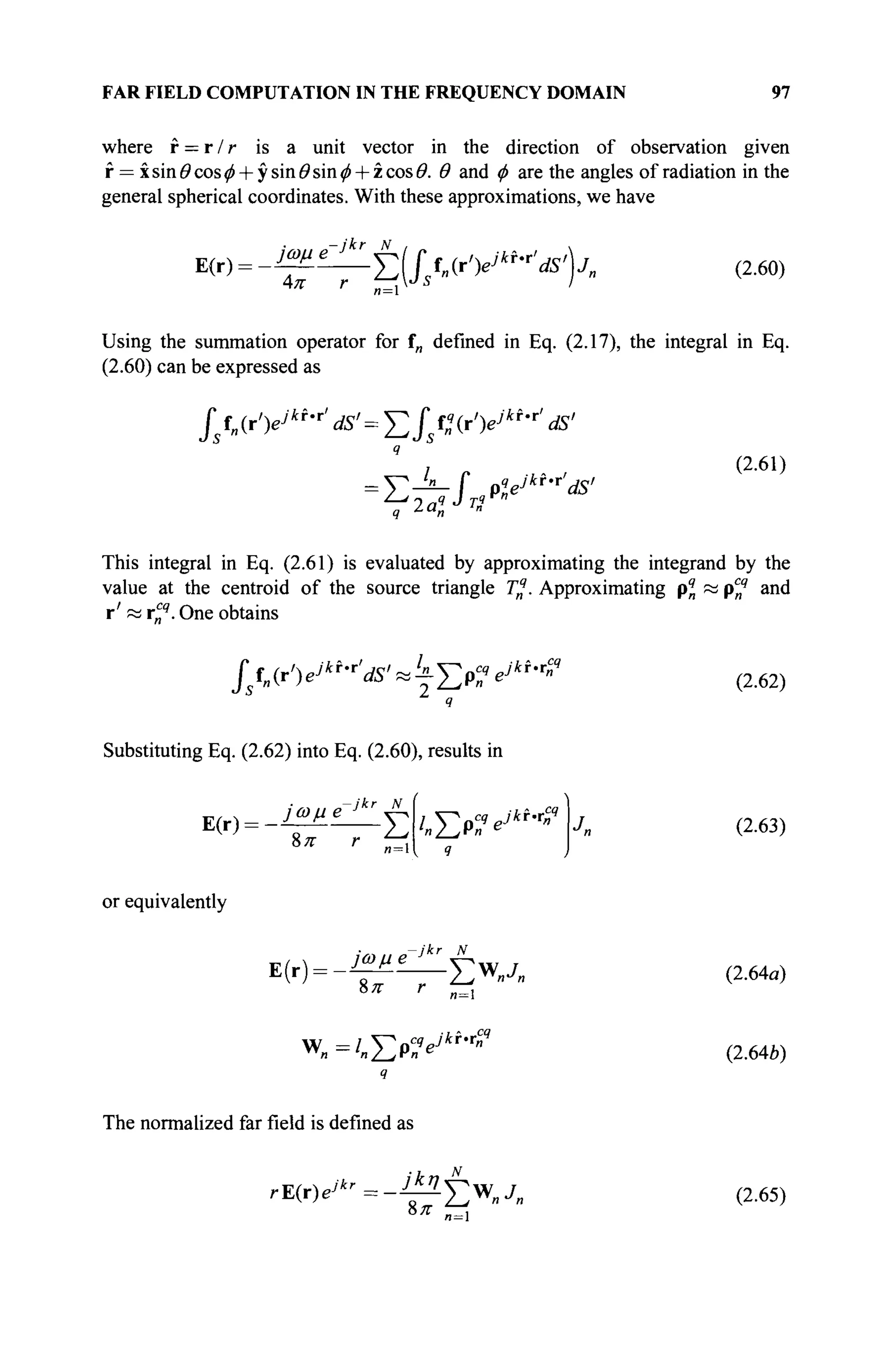
![98 ANALYSIS OF CONDUCTING STRUCTURES IN THE FREQ DOMAIN
where the parameter к is the wave number and the parameter η is the intrinsic
impedance of the medium surrounding the scatterer.
Numerical results using these formulations will be presented in Chapter
4.
2.9 CONCLUSION
Analysis of the electromagnetic scattering by arbitrarily shaped conducting objects
in the frequency domain is presented in this chapter Method of Moment,
triangular surface patch modeling and the RWG basis functions have been used to
solve the electric field integral equation, the magnetic field integral equation, and
the combined field integral equation. Of them, the EFIE can be used for both open
and closed objects, whereas the MFIE and the CFIE is used only for closed
surfaces. Numerical examples using these formulations for the analysis of
composite conducting and dielectric structures will be presented in Chapter 4.
REFERENCES
[1] Y. Zhang, and T. K. Sarkar, Parallel Solution of Integral Equation-based EM
Problems in the Frequency Domain, John Wiley & Sons, New York, 2009.
[2] S. M. Rao, D. R. Wilton, and A. W. Glisson, "Electromagnetic scattering by
surfaces of arbitrary shape," IEEE Trans. Antennas Prop., Vol. 30, pp. 409^18,
1982.
[3] S. M. Rao, Electromagnetic Scattering and Radiation of Arbitrarily-Shaped
Surfaces by Triangular Patch Modeling, PhD Dissertation, University Mississippi,
August, 1980.
[4] D. R. Wilton, S. M. Rao, A. W. Glisson, D. H. Schaubert, О. M. Al-Bundak, and С.
M. Butler, "Potential integrals for uniform and linear source distributions on
polygonal and polyhedral domains," IEEE Trans. Antennas Prop., Vol. 32, pp.
276-281, 1984.
[5] A. J. Poggio and E. K. Miller, "Integral equation solutions of three dimensional
scattering problems," Computer Techniquesfor Electromagnetics, Pergamon Press,
New York, 1973.](https://image.slidesharecdn.com/timeandfrequencydomainsolutionsofemproblemsusingintegralequationsandahybridmethodologyb-250205130750-568a5ba2/75/Time-and-Frequency-Domain-Solutions-of-EM-Problems-Using-Integral-Equations-and-a-Hybrid-Methodology-B-H-Jung-pdf-120-2048.jpg)
![3
ANALYSIS OF DIELECTRIC OBJECTS
IN THE FREQUENCY DOMAIN
3.0 SUMMARY
In this chapter, numerical methods used to analyze the electromagnetic scattering
from three-dimensional (3-D) homogeneous dielectric bodies of arbitrary shapes in
the frequency domain are addressed. Five different integral equation formulations
are described here, viz. the electric field integral equation (EFIE), the magnetic
field integral equation (MFIE), the combined field integral equation (CFIE), the
Poggio-Miller-Chang-Harrington-Wu integral equation (PMCHW), and the
Müller integral equation. The EFIE and MFIE are derived using the boundary
conditions of the electric or the magnetic field, respectively, whereas the other
equations consider both boundary conditions. In addition, a thorough study on
different combinations of the testing functions in the CFIE and the Müller
equation are presented. It is demonstrated that not all CFIE formulations are
accurate enough in removing defects that occur at frequencies corresponding to an
internal resonance of the structure. At the end of this chapter, the equivalent
electric current, magnetic current, far scattered field, and radar cross-section
(RCS) are computed based on the described formulations for three dielectric
scatterers of different shapes, viz. a sphere, a cube, and a finite circular cylinder.
Through the comparison of these results, the effectiveness of different
formulations is illustrated.
3.1 INTRODUCTION
This section deals with the scattering from arbitrarily shaped 3-D homogeneous
dielectric bodies in the frequency domain. Furthermore, the simpler EFIE or MFIE
formulations fail at certain discrete frequencies that correspond to the internal
resonances of the structure. One possible way to obtain a unique solution at an
internal resonant frequency of the structure under analysis is to combine a
weighted linear sum of the EFIE with MFIE and thereby minimize the effects of
spurious solutions [1]. The CFIE, as the name implies, is a combination of EFIE
and MFIE. The use of a combined field formulation does not eliminate the
99
Time and Frequency Domain Solutions of EM Problems
Using Integral Equations and a Hybrid Methodology
by B. H. Jung, T. K. Sarkar, S. W. Ting, Y. Zhang, Z. Mei, Z. Ji,
M. Yuan, A. De, M. Salazar-Palma, and S. M. Rao
Copyright © 2010 John Wiley & Sons, Inc.](https://image.slidesharecdn.com/timeandfrequencydomainsolutionsofemproblemsusingintegralequationsandahybridmethodologyb-250205130750-568a5ba2/75/Time-and-Frequency-Domain-Solutions-of-EM-Problems-Using-Integral-Equations-and-a-Hybrid-Methodology-B-H-Jung-pdf-121-2048.jpg)
![100 ANALYSIS OF DIELECTRIC OBJECTS IN THE FREQ DOMAIN
problem of the internal resonances; it merely pushes them off the real frequency
axis into the complex s-plane, thereby minimizing the effects of the spurious
modes when observed along the real frequency axis. Although an integral equation
formulation has been used for analyzing 3-D dielectric bodies in the frequency
domain, only a few researchers have applied it to the analysis of scattering by
arbitrarily shaped 3-D objects with triangular patch modeling [2-9].
The PMCHW formulation was proposed [2,5], in which Rao-Wilton-
Glisson (RWG) functions have been used as both the basis and the testing
functions, and also to approximate both the electric and the magnetic currents.
However, a similar scheme, when used to solve the EFIE or MFIE, yielded ill-
conditioned matrices and inaccurate results. To overcome these problems for the
EFIE formulation, the electric current is expanded using the RWG functions,
whereas the magnetic current is expanded using another set of basis functions
given by nxRWG, which are pointwise spatially orthogonal to the RWG set [3].
Here, n is the unit normal pointing outward from the surface. In addition, the
RWG basis functions are also used as the testing functions. Next, Rao and Wilton
proposed the CFIE along with EFIE and MFIE for the analysis of scattering by
arbitrarily shaped 3-D dielectric bodies for the first time [4]. In their work, RWG
functions are used to approximate the electric current, but the magnetic current is
approximated by nxRWG [3], and a line testing is used. In a recent paper [6],
Sheng et al. proposed a CFIE formulation for the same problem. In Sheng's work,
the RWG functions are used as basis functions to approximate both the electric and
magnetic currents, and a linear combination of RWG and n x RWG functions are
used as testing functions. This yields a well-conditioned matrix. Sheng also
presented a set of four CFIE formulations by dropping one of the testing terms in
(RWQ EFIE) + ( n x RWG EFIE) + (RWG MFIE) + ( n x RWG MFIE).
For the Müller's formulation, the equivalent currents are expanded using
the RWG functions, and a combination of the RWG functions and its orthogonal
component is used for testing. All possible cases of the testing procedure are
investigated using the four parameters in conjunction with the testing functions.
Further, a new set of pulse basis functions on triangular patches was used to solve
the EFIE, MFIE, and CFIE formulations [10]. In this chapter, various integral
formulations are investigated and several combinations of CFIE are proposed with
different choices of testing functions. The results illustrate that not all CFIE
formulations are stable.
This chapter is organized as follows. In section 3.2, the integral equations,
EFIE, MFIE, CFIE, PMCHW, and the Müller equation are introduced and the
different testing and basis functions are discussed in section 3.3. Numerical
procedures to solve them are given in sections 3.4-3.8. The evaluation of various
integrals appearing in these numerical solutions is given in the appendix at the end
of this chapter. Section 3.9 presents the accuracy comparison of using several
formulations of CFIE, and section 3.10 provides the Muller's formulations. In
section 3.11, more than 30 numerical results for the analysis of a dielectric sphere,
a cube, and a finite circular cylinder using different formulations are presented and
compared with the Mie series solution and the available software—HOBBIES
(higher order basis function based integral equation solver) [11]. Finally, some
conclusions are presented in section 3.12](https://image.slidesharecdn.com/timeandfrequencydomainsolutionsofemproblemsusingintegralequationsandahybridmethodologyb-250205130750-568a5ba2/75/Time-and-Frequency-Domain-Solutions-of-EM-Problems-Using-Integral-Equations-and-a-Hybrid-Methodology-B-H-Jung-pdf-122-2048.jpg)
![INTEGRAL EQUATIONS 101
3.2 INTEGRAL EQUATIONS
In this section, the mathematical steps are described to obtain the integral
equations to analyze the electromagnetic scattering by arbitrarily-shaped 3-D
homogeneous dielectric bodies. To simplify the presentation, the formulations are
only presented for a single dielectric body, and it is possible to extend this
formulation for handling multiple dielectric bodies.
Consider a homogeneous dielectric body with permittivity ε2 and
permeability μ2 placed in an infinite homogeneous medium with permittivity εχ
and permeability μ1 as shown in Figure 3.1. A lossy material body can be handled
by considering ε2 , μ2 to be complex quantities. Throughout this chapter, the
subscripts 1 and 2 are used to represent the region outside and inside the dielectric
body to be studied, respectively. The structure is now illuminated by an incident
plane wave denoted by (Ε', Η' ). It may be noted that the incident field is defined
to exist if the structure were not present. By invoking the equivalence principle
[12], the following two relations corresponding to the exterior and interior regions
are formed in terms of the equivalent electric current J and the magnetic current M
on the surface S of the dielectric body.
Figure 3.1. Homogeneous dielectric body illuminated by an electromagnetic plane wave.
While applying the equivalence principle for the region external to the body, the
field in the interior region is set to zero and the entire interior space is filled by the
homogeneous medium (εχ, μχ) which was originally external to the body only.
As a result, the whole problem space is filled with a homogeneous medium
allowing us to use the free space Green's function to calculate the fields.
Equivalent electric and magnetic currents, J and M, are then placed on the surface
of the body to preserve the continuity of the fields across the dielectric boundary.
By enforcing the continuity of the tangential electric and magnetic field at S_,
where S_ is selected to be slightly interior to S, we obtain
(-Ef(J,M)) = ( E ' ) (3.1)
V /tan V /tan v
'](https://image.slidesharecdn.com/timeandfrequencydomainsolutionsofemproblemsusingintegralequationsandahybridmethodologyb-250205130750-568a5ba2/75/Time-and-Frequency-Domain-Solutions-of-EM-Problems-Using-Integral-Equations-and-a-Hybrid-Methodology-B-H-Jung-pdf-123-2048.jpg)
![102 ANALYSIS OF DIELECTRIC OBJECTS IN THE FREQ DOMAIN
(-Hi(J.M)) =(№') (3.2)
V /tan /tan v
'
where the subscript 1 indicates that the scattered field (Ef, Hj ) is computed in the
external region. Using similar procedures for the interior region, the fields in the
region external to the body are set to zero and thus, the external region is replaced
by the material ( ε2 , μ2) so that the currents are entirely located in a
homogeneous medium, which was originally inside the dielectric body only. By
enforcing the continuity of the tangential electric and magnetic fields at S+, where
S+ is the surface slightly exterior to S,the following equations are derived:
(-E5(J,M))t m =0 (3.3)
(-1ВДМ)) = 0 (3.4)
v /tan
where the subscript 2 indicates that the scattered field (E2, Hs
2 ) is computed in the
internal region. In Eqs. (3.1)—(3.4), the subscript 'tan' refers to the tangential
component of the fields only. Because both the internal and external problems are
formulated in terms of the electric current J and the magnetic current M radiating
in respective homogeneous mediums, the scattered electric and magnetic fields
caused by these currents can be expressed analytically as
Et(J) = -yû>A„-V<Pv (3.5)
E*(M) = - — VxFy (3.6)
H*(J) = — VxAv (3.7)
Ηΐ(Μ) = -]ω¥ν-νΨν (3.8)
In Eqs. (3.5)-(3.8), the symbol v is used to represent the region in which the
currents J or M are radiating and can be assigned as either 1 for the exterior region
or 2 for the interior region. The parameters Av , F„ , Φν, and Ψν are the magnetic
vector potential, electric vector potential, electric scalar potential and magnetic
scalar potential, respectively, which are explicitly given by
Av(r) = ^ f j ( r ' ) G v ( r , r V 5 ' (3.9)
ЕДг) = - ^ Г M(r')G„(r, r')dS' (3.10)](https://image.slidesharecdn.com/timeandfrequencydomainsolutionsofemproblemsusingintegralequationsandahybridmethodologyb-250205130750-568a5ba2/75/Time-and-Frequency-Domain-Solutions-of-EM-Problems-Using-Integral-Equations-and-a-Hybrid-Methodology-B-H-Jung-pdf-124-2048.jpg)
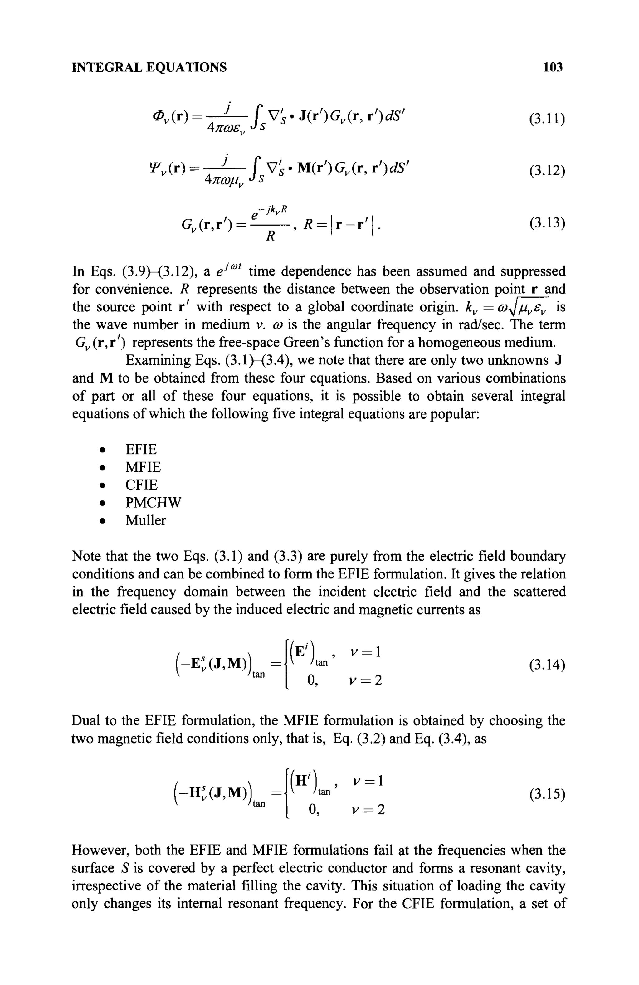
![104 ANALYSIS OF DIELECTRIC OBJECTS IN THE FREQ DOMAIN
two integral equations are formed from the linear combination of EFIE in Eq.
(3.14) and MFIE in Eq. (3.15) by using the following form:
к (-К (J, M)) + (1 - к) щ (-H* (J, M))
/tan /tan
кЫ + ( 1 - * W H ' ' ) , ν = (3.16)
— V /tan V /tan
0, v = 2
where ηχ is the wave impedance of the exterior region and к is a scale factor
between 0 and 1. An alternative way to combine the four equations, Eq. (3.1) to
(3.4), is the PMCHW formulation. In this formulation, the set of four equations is
reduced to two by adding Eq. (3.1) to Eq. (3.3) and Eq. (3.2) to Eq. (3.4), giving
(-Щ(3,М)-Ц(ЗМ))ш=(*)ш (3.17α)
(-Hi(J,M)-Hs
2 (J,M)) = ( н ' ) (3.17b)
/tan V /tan
In addition, the PMCHW equations can be extended in Eq. (3.17) by introducing
two more parameters a and β as
(-Ei(J,M)-aE'2 (J,M)) =(E'') (3.18a)
V /tan V /tan
(-HÎ(J,M)-^H5(J,M)) =(Н') (3.18i)
/tan V /tan
where α = ει/ε2 and β = μλ/μ2. This is called the Müller formulation [1]. The
Müller equation is same as the PMCHW formulation when a = ß = 1.
3.3 EXPANSION AND TESTING FUNCTIONS
For any one of the integral equations mentioned previously, note that there are the
two unknowns, J and M, and they can be determined by using similar MoM
numerical procedures introduced in Chapter 2. First, the dielectric object is
assumed to be a closed body and modeled by the planar triangular patches. Next,
the unknown currents J and M need to be expanded with suitable basis functions,
and tested with the suitable testing functions. In the following, we define two sets
of functions that may be useful. The first is the RWG functions defined in Chapter
2. As noted earlier, the RWG vector function associated with the nth edge is given
by
f„(r) = f„+(r) + f;(r) (3.19a)](https://image.slidesharecdn.com/timeandfrequencydomainsolutionsofemproblemsusingintegralequationsandahybridmethodologyb-250205130750-568a5ba2/75/Time-and-Frequency-Domain-Solutions-of-EM-Problems-Using-Integral-Equations-and-a-Hybrid-Methodology-B-H-Jung-pdf-126-2048.jpg)
![EXPANSION AND TESTING FUNCTIONS 105
UM-
l
" PÎ, r e î f
2a, (3.1%)
0, r?7?
and the surface divergence of Eq. (3.19) is
Vs .f„(r) = Vs.f„+
(r) + Vs.f„-(r)
Vs.f,f(r) =
±Α_ re г*
<3И
0, r ^
(3.20a)
(3.206)
In Eqs. (3.19) and (3.20), /„ is the length of the nonboundary edge and a+ and
a~are the areas of the triangles T^ and T~, respectively. Vectors p* and p~ are
the position vectors defined with respect to the free vertices of Γ„+
and T~.
Next, we define another vector basis function g„ that is point-wise
orthogonal to the RWG function fn in the same triangle pair, given by
g„(r) = nxf„(r) (3.21)
where n is the unit normal pointing outward from the surface [3]. These two sets
of functions are used in several different ways to solve five integral equations
defined earlier. The various choices of the expansion and testing functions for the
electric and magnetic currents in the five formulations, EFIE, MFIE, CFIE,
PMCHW, and the Müller equation, are summarized in Table 3.1. The reason for a
specific choice will be discussed in the following sections.
Table 3.1. Expansion and Testing Functions in Different Formulations
Formulation
EFIE
MFIE
CFIE
PMCHW
Müller
Testing function
f»
+ f„ + g„
tm
+ U + g„
Current
J
f„
%n
in
in
fn
expansion function
M
g«
f.
f„
f„
f„
Next, the numerical procedures to solve the various integral equations
using the method of moments (MoM) methodology are outlined.](https://image.slidesharecdn.com/timeandfrequencydomainsolutionsofemproblemsusingintegralequationsandahybridmethodologyb-250205130750-568a5ba2/75/Time-and-Frequency-Domain-Solutions-of-EM-Problems-Using-Integral-Equations-and-a-Hybrid-Methodology-B-H-Jung-pdf-127-2048.jpg)
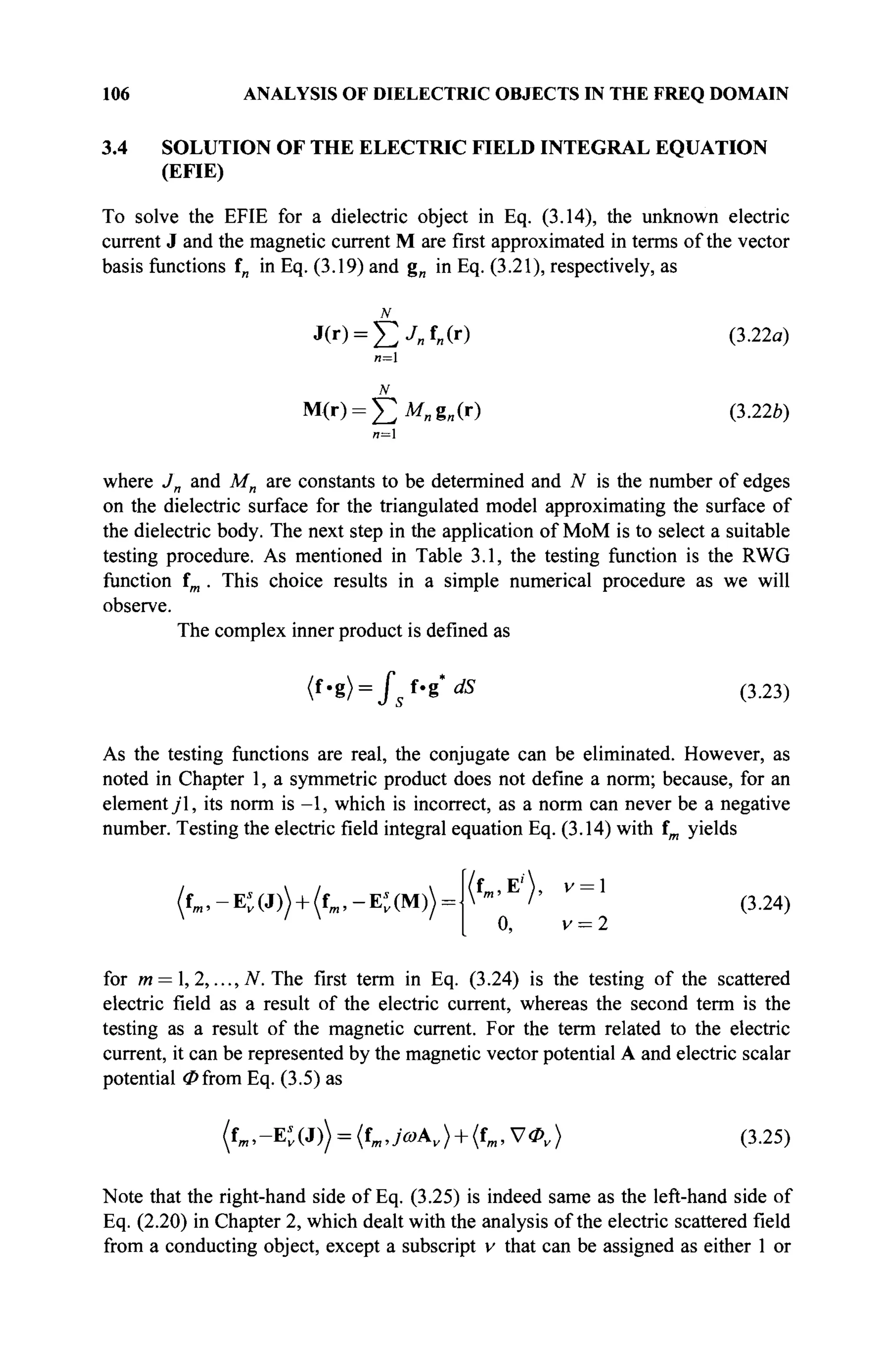
![SOLUTION OF THE EFIE 107
2 is added to indicate the region where the fields are considered. Meanwhile, the
unknown electric current J is expanded by the basis function in in both Eqs.
(3.25) and (2.20). The detailed steps of the derivation are available in [4,5]. When
the testing of Eq. (2.29) is applied, one obtains
N
i N
f«. -Ev(J)> = m E V A - — Σ 5
™ , ' · 7
« (3.26α)
' „=l ωε
ν „=l
where
4,»,, =-^Jstm(r)'Jstn(r')Gv(r,r,
)dS,
dS (3.26b)
B
^v=~Î^S^m{r)jV's'i„{r')Gv{r,r')dS'dS (3.26c)
Now examine the second term in Eq. (3.24) that describes the scattered
electric field caused by the magnetic current. Extracting the Cauchy principal
value from the curl term on a planar surface in Eq. (3.6) and using Eq. (3.10), the
following can be written:
-Et(M) = — VxFK(r) = ± ^ n x M ( r ) +—VxF„(r) (3.27)
εν 2 εν
where Fv is defined by Eq. (3.10) with the removal of the singularity at r = r' (or
R = 0) from the integration. In Eq. (3.27), the positive sign is used when v = 1
and negative sign is used when v = 2. Therefore, by substituting Eq. (3.27), the
second term of Eq. (3.24) is now rewritten as
(fm ,-Et(M)) = ( f „ , ± ± n x M + /fm,— VxFv (3.28)
The magnetic current M in the first term on the right-hand side of Eq. (3.28) can
be replaced by the expansion function defined in Eq. (3.22b)
1 N
f m , ± - n x M = Σ Χ „ ν Μ „ (3.29α)
n=l
where
iji fm (r).nxgl ,(r)dS> v = l
r f fm(r).nxg„(r)J5, v = 2
г (3.29b)
2Js](https://image.slidesharecdn.com/timeandfrequencydomainsolutionsofemproblemsusingintegralequationsandahybridmethodologyb-250205130750-568a5ba2/75/Time-and-Frequency-Domain-Solutions-of-EM-Problems-Using-Integral-Equations-and-a-Hybrid-Methodology-B-H-Jung-pdf-129-2048.jpg)
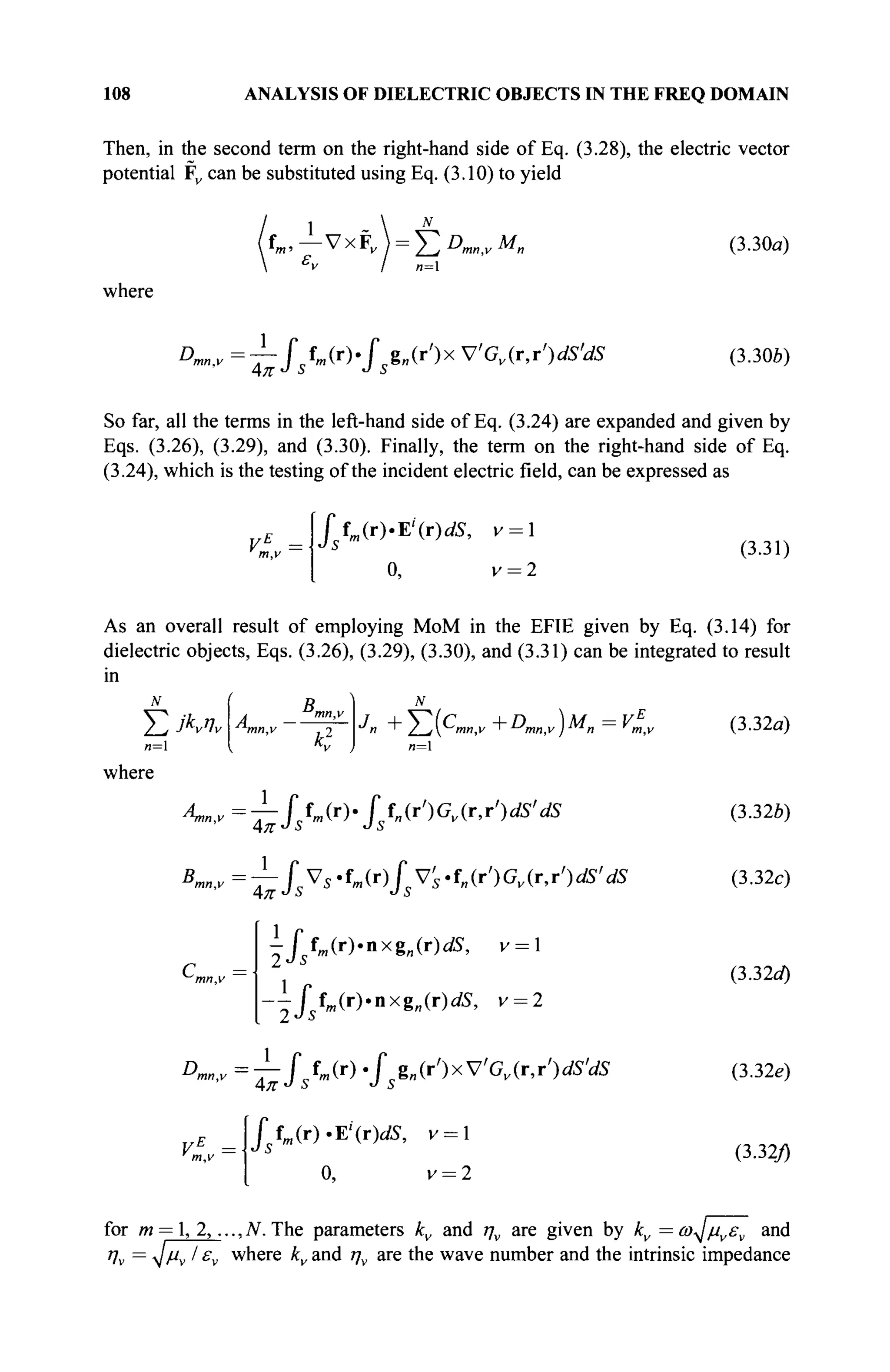
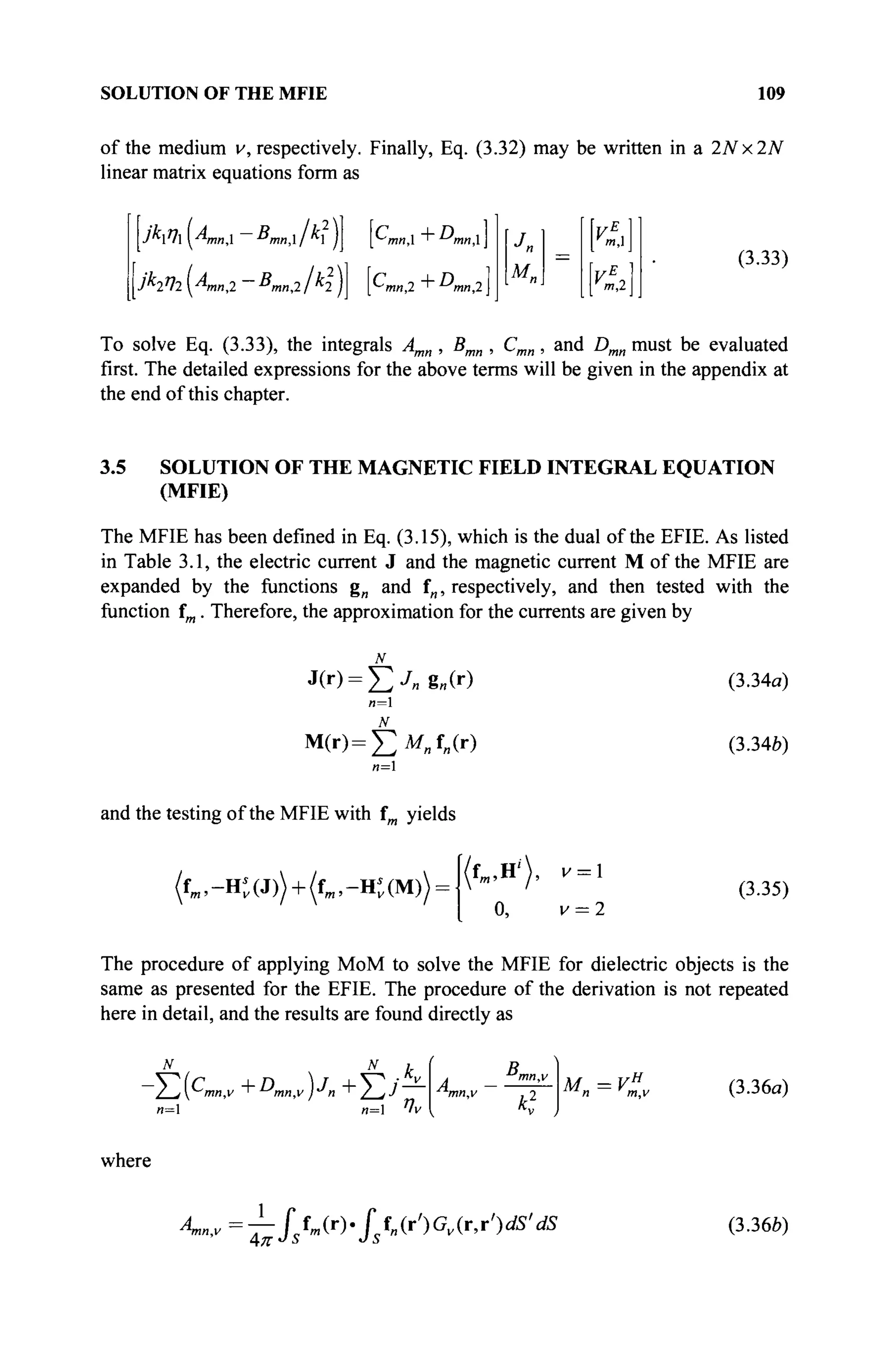
![по ANALYSIS OF DIELECTRIC OBJECTS IN THE FREQ DOMAIN
B^v~fsVs-tm(r)fsVs-f„(r')Gv(r,r')dS'dS
1
fsfm(r).nxg„(r)dS, v =
l
-ffm(r)4ixgn(r)dS, v = 2
г =
2Js
" f
Dm„,v =±-f sîm(r).f sg„(r')xVGv(ry)ciS' dS
'Jsfm(r).H''(r)dS, v =
0, v = 2
VH
=
(3.36c)
(3.36a)
(3.36e)
(3.36/)
The integrals Amnv , Bmnv , Cmnv , and Dmnv are the same as those in Eq. (3.32).
Note that Eq. (3.36) can also be obtained directly from EFIE in Eq. (3.32) by using
the principle of duality [8]. Similarly, Eq. (3.36) is associated with each edge, and
it may be written in a matrix form for m = , 2,..., N as
-C — Г)
*-Ίηη,1 1J
mn
JKIT
lAmn, Bmn, A.2
)
M„]
m,
■ H
(3.37)
Eq. (3.37) is a 2Nx2N linear equations in matrix form. Solving the currents Jn
and Mn in this matrix equation can lead to the determination of the scattered field.
3.6 SOLUTION OF THE COMBINED FIELD INTEGRAL EQUATION
(CFIE)
For the CFIE formulation, we note that it is not possible to simply combine the
EFIE and the MFIE solutions described in the previous two sections. The primary
difficulty is the expansion functions for J and M are not the same in both
formulations. Hence, we adapt the following procedure.
Here, the basis function in is used to expand both J and M as
J(r) = £ j „ f „ ( r ) (3.38a)
n=
Μ(Γ)=£>Λ(Γ) (3.38b)
n=](https://image.slidesharecdn.com/timeandfrequencydomainsolutionsofemproblemsusingintegralequationsandahybridmethodologyb-250205130750-568a5ba2/75/Time-and-Frequency-Domain-Solutions-of-EM-Problems-Using-Integral-Equations-and-a-Hybrid-Methodology-B-H-Jung-pdf-132-2048.jpg)
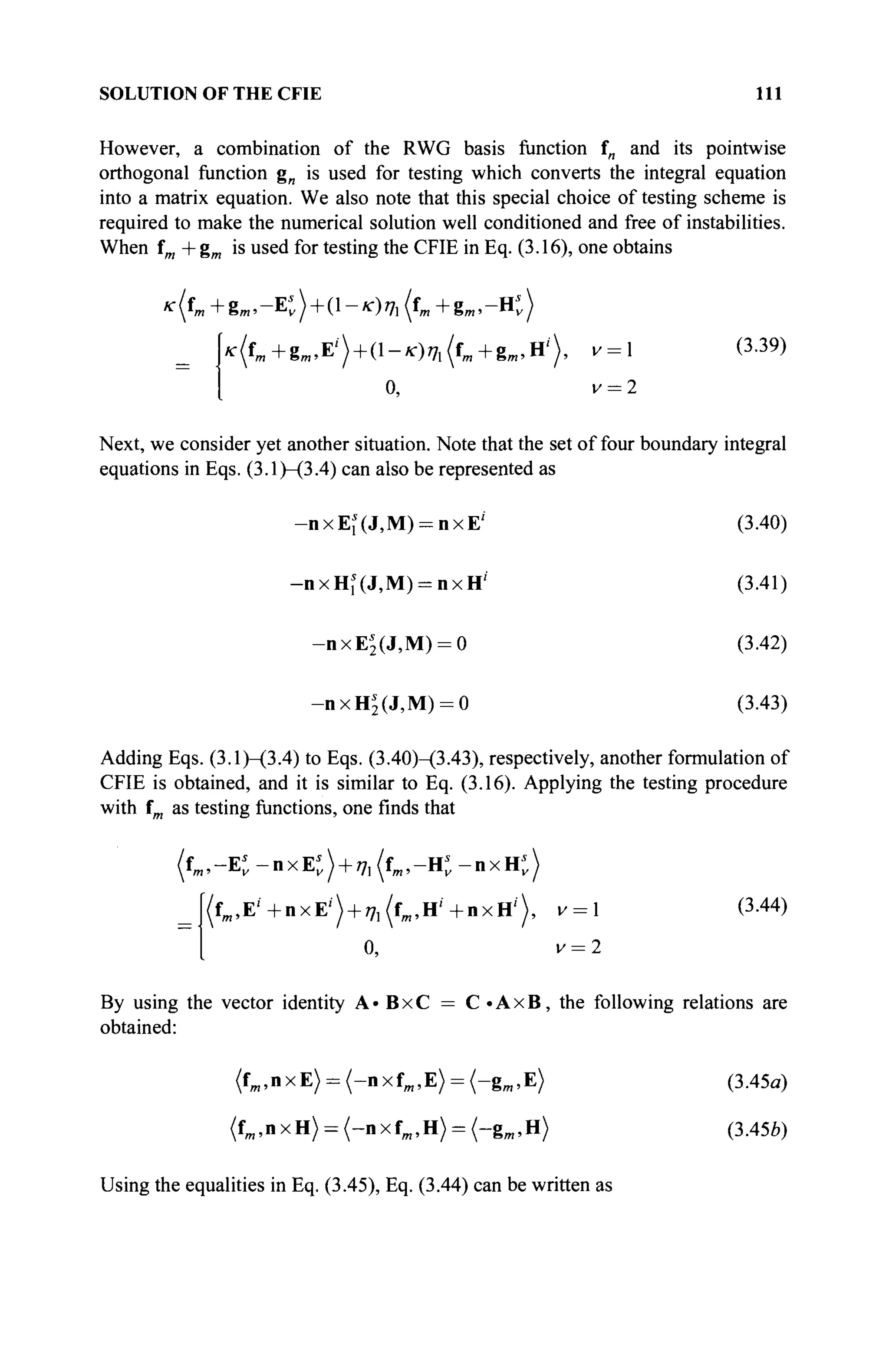
![112 ANALYSIS OF DIELECTRIC OBJECTS IN THE FREQ DOMAIN
*(«'m-g».-Et)+(l-*)7i(fB ,-gB „-Ht)
>c(fm -gffl,E'') + ( l - ^ ) ^ (fm -g l B ,H'), к = 1
0, v = 2
(3.46)
It is important to note that the testing function is fm +gm in Eq. (3.39) and
fm —gm in Eq. (3.46) for the same CFIE. This implies that fm + gm or fm — gm
can be used to test either the part of EFIE or MFIE, and this may result in eight
different CFIE combinations as (fm ±gm ,E)±(fm ±gm ,H). For this, the
expression for CFIE is generalized by involving four parameters,
fE, gE, fH,andgH, in conjunction with the testing functions as
{l-K){fEtm+8ESm,-K) + nh(fHtm+gHim,-K)
(1 - *) (fEtm + «£gm.E
' ) + "Й {/HL + ёнЪт , H'' ), V = 1
0, ν = 2
(3.47)
where /с is a parameter for linear combination that can have any value between 0
and 1. The testing coefficients fE, gE, fH, and gH may be either +1 or — 1. If
/E = 8E =
/H =
8H =
1 ' ш е п
Eq· (3.47) is the same as Eq. (3.39), or it becomes
Eq. (3.46) when fE = fH = 1 and gE = gH = -1.
To transform Eq. (3.47) into a matrix equation, this equation is divided
into two parts: the electric field and the magnetic field parts. For the part related to
the electric field only, we have
(fEfm+gEgm,-K(*№)
(/£f»+Ä£g«»E'),
°.
v = l
v = 2
(3.48)
This equation is called the TENE formulation [6] in which ТЕ stands for the
testing of the electric field with the tangential function fm and NE denotes that
with the normal function gm.Thus, by using a similar procedure as in EFIE, we
have
N
ΣίΚΐν
n=
Bi I
·*n T / j^mn.v "+" Umnv J Mn = Vmv
n=
(3.49a)
where
mn,v JE mn,v ' 6E-™mn,v
mn,v JE mn,v ' o£ mn,v
(3.49Ô)
(3.49c)](https://image.slidesharecdn.com/timeandfrequencydomainsolutionsofemproblemsusingintegralequationsandahybridmethodologyb-250205130750-568a5ba2/75/Time-and-Frequency-Domain-Solutions-of-EM-Problems-Using-Integral-Equations-and-a-Hybrid-Methodology-B-H-Jung-pdf-134-2048.jpg)
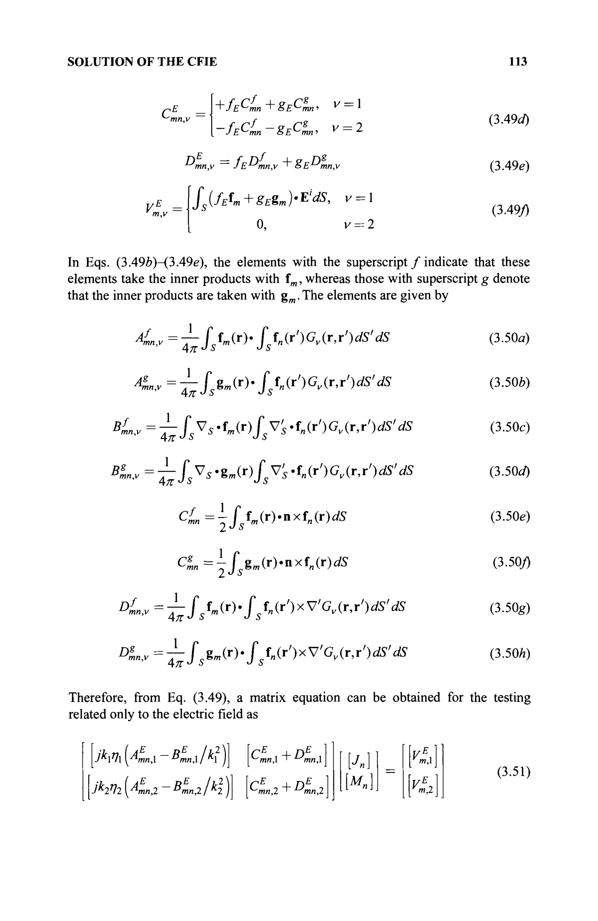
![114 ANALYSIS OF DIELECTRIC OBJECTS IN THE FREQ DOMAIN
Next, we write the testing equation corresponding to the magnetic field only from
Eq. (3.47) as
(fHfm+gHgm,-Hs
v(J,M)
0, v = 2
(3.52)
This equation is called the THNH formulation [6] in which TH stands for the
testing to the magnetic field with the tangential function f„ and N H denotes that
with the normal function gm .Thus, by using a similar procedure as in the MFIE,
the following is obtained
и=1 n= ^v
.H D
mn,
mn,v 2
M = V (3.53α)
where
Ληη,ν — /нАпп,у +8нАпп,у
Β/ηη,ν =
JH^mn,v + SH^mn.v
Сн
=-!
+fHc
L+gHc
L· v= 1
—
/яЧл« ~ ёнСтп' V = 2
VH
m.v
/5 (//Л,+£я8т)-Н'<0, V =
0, v = 2
(3.536)
(3.53c)
(3.53rf)
(3.53e)
(3.53/)
In Eqs. (3.536)-(3.53e), the elements with superscripts / and g are the same as
those in Eqs. (3.50). Note that Eq. (3.53) can be obtained directly from Eq. (3.49)
by using duality. The matrix equation corresponding to Eq. (3.53) is given by
(QM,I + DmnX )J jkx /ηχ ^AmnX BmnX I kx
A/%K„,2-^,2 A2
2
)]
~(Cm«,2 D"2)
m,
m,2
(3.54)
The matrix equations Eq. (3.51) and Eq. (3.54) are rewritten, respectively, as
K
zH
c 1
(3.55a)
(3.55b)](https://image.slidesharecdn.com/timeandfrequencydomainsolutionsofemproblemsusingintegralequationsandahybridmethodologyb-250205130750-568a5ba2/75/Time-and-Frequency-Domain-Solutions-of-EM-Problems-Using-Integral-Equations-and-a-Hybrid-Methodology-B-H-Jung-pdf-136-2048.jpg)
![SOLUTION OF THE PMCHW INTEGRAL EQUATION 115
where C„ = J„ and С(ЛГ+и) = Mn for n = l,2,...,N. Finally, by combining
TENE and THNH, as given in Eqs. (3.55a) and (3.55è), a matrix equation is
formed for the general CFIE testing equation given by Eq. (3.47), which is termed
TENE-THNH, as
Kn][Cn] = [Vm] (3.56a)
where the matrix elements are given by
Ζιαα=(ΐ-κ)Ζ^+κηιΖ^, (3.56ft)
Ут={-кУ1+щхУ» (3.56с)
for m = 1, 2,..., 2N and n — 1, 2, ..., 2Ν. To solve the previous matrix
equation, it is required that the integrals Af
mn , Bf
mn , Cf
mn, Df
mn , Α*„ , Βξ,η , Cs
mn,
and D^n are determined first. The formulations of applying the RWG basis
function on the triangular patches for approximating these integrals is given in the
appendix at the end of this chapter.
3.7 SOLUTION OF THE PMCHW INTEGRAL EQUATION
For the PMCHW formulation of Eq. (3.17), the expansion functions for both the
electric current J and the magnetic current M are f„ as that in the CFIE given by
Eq. (3.38); and the testing function is fm. Applying the testing procedure to Eq.
(3.17) yields
(fm ,-Ei(J,M)) + (fm,-E^(J,M)) = (fm,E') (3.57a)
(fm ,-HKJ,M)) + (fm>-H*2(J,M))= (fm,H') (3.57ft)
Eq. (3.57) contains two testing equations in which Eq. (3.57a) is related only to
the electric field and Eq. (3.57ft) is for the magnetic field. First, let us look at Eq.
(3.57a) and compare it with the testing of EFIE in Eq. (3.24). It can be observed
that they have a similar form, except Eq. (3.57a) includes the testing of both the
scattered electric fields Ej and E2 . Therefore, the result from applying MoM can
be derived by adding the EFIE results in Eq. (3.33) for these two fields.
Furthermore, the expansion function for M is now f„ and is different from g„ in
the EFIE; thus, the formulation for the PMCHW has to be modified, mainly in the
integrals Cmnv and Dmnv. The integral Cmnv becomes zero in the PMCHW
formulation because, for regions 1 and 2, the terms are negative of each other and
when combined, yield zero value. Also, for the integral Dmn v , one needs to
replace the term g„ with fn . The result is given by](https://image.slidesharecdn.com/timeandfrequencydomainsolutionsofemproblemsusingintegralequationsandahybridmethodologyb-250205130750-568a5ba2/75/Time-and-Frequency-Domain-Solutions-of-EM-Problems-Using-Integral-Equations-and-a-Hybrid-Methodology-B-H-Jung-pdf-137-2048.jpg)
![116 ANALYSIS OF DIELECTRIC OBJECTS IN THE FREQ DOMAIN
N 2
Σ Σ JKvv
n= v=
Bm
N 2
ΣΣ
Jn+Ï2Î2D
n».vM
x=V
m
Am„,v=—Jtm(T)'Jfn(r')Gv(T,r')dS'dS
B„
D.
1
fsVs-fm(r)fsVs'f„(r')Gv(r,r')dS'dS
^fsfm(r).fsfn(r')xV'Gv(r,r')dS'dS
V„ = / s f m ( r ) . E ' ( r ) ^
4π Js
1
(3.58a)
(3.58*)
(3.58c)
(3.58a)
(3.58e)
In Eq. (3.58), Amnv and Bmnv are the same as those used for the EFIE in Eq.
(3.32).
Consider the testing in Eq. (3.57b) and compare it with the testing of
MFIE in Eq. (3.35); one can find that they have the same form, except Eq. (3.576)
includes both the testing of the scattered magnetic fields Hj and Hs
2 . Therefore,
one can directly apply the result of MFIE in Eq. (3.36) for these two fields and
sum them together. Also the integral Cmnv becomes zero, and the vector function
g„ in the integral Dmnv has to be replaced by fn. The result can be expressed as
N2 N 2 t
Л Д
" " И
мп = v% (3.59a)
where
^ ' v =
Г ~ ] Л ( Г )
· is^')Gv(T,r')dS'dS
Bmn,v~fsVS-tm(r)fVs-fn(r')Gv(r,r')dS'dS
D„ -^fstm(r)'fsf„(r')xVGv{r,r')dS'dS
Vf = Jsfm(r)-n'{r)dS
(3.59b)
(3.59c)
(3.59o)
(3.59e)
The integrals Amnv , Bmnv , and Dmnv are the same as those in Eq. (3.58),
respectively. Note that Eq. (3.59) can be obtained directly from Eq. (3.58) by
using duality without any additional effort. Equation (3.58) and Eq. (3.59) are
associated with each edge, where m = 1, 2,..., N . Therefore, a matrix equation
can be obtained as](https://image.slidesharecdn.com/timeandfrequencydomainsolutionsofemproblemsusingintegralequationsandahybridmethodologyb-250205130750-568a5ba2/75/Time-and-Frequency-Domain-Solutions-of-EM-Problems-Using-Integral-Equations-and-a-Hybrid-Methodology-B-H-Jung-pdf-138-2048.jpg)
![SOLUTION OF THE MULLER INTEGRAL EQUATION 117
Σ Λ ^
v=
4 _ B m
" · '
mn,v j 2
v=l
_2
i/~l
/ jmn.v
v= Ίν
B„
à - mn,v
mn2 t n
M„]
(3.60)
3.8 SOLUTION OF THE MÜLLER INTEGRAL EQUATION
The last formulation to be introduced is the Müller integral equation. It was first
introduced in Eq. (3.18). Note that it becomes the PMCHW formulation when
а = ß = 1. Similar to CFIE and PMCHW, the RWG function f„ is chosen as the
expansion functions for both the electric current J and the magnetic current M, as
given by Eq. (3.38). The testing function selection follows the same procedure as
CFIE. In the CFIE formulation, Eq. (3.47), a combination of RWG function fn and
its orthogonal component g„ = n x f„, is used as the testing function to convert the
integral equation into a matrix equation.
Now consider the testing procedure for the Müller equation. By
substituting Eqs. (3.5)-(3.8) into Eqs. (3.18) and extracting the Cauchy principal
value from the curl term, Eq. (3.18) can be rewritten as
7'ω(Α, +ccA2) + V(0l +αΦ2 ) + ( 1 - α ) - η χ Μ
+PV
1 „ „ 1 „ „
— V x F , + a — V x F 2
:(E<) (3.61a)
>(F, +β¥2) + V(f, + βΨ2)-{-ß)-nxi
-PV -VxA, +ß—VxA2
[Mi Mi
:(H<) (3.616)
where PV denotes the principal value. In the PMCHW formulation, when
а = ß = 1, the third terms in Eqs. (3.61a) and (3.6le) are dropped out. In this
PMCHW integral equation, an accurate and stable solution can be obtained by
using the RWG function fn as the testing functions [2,6,13]. To test the third
terms nxM and n x J in Eq. (3.61), the spatially orthogonal component gm is
applied to the Müller equation. Now, a general expression is presented for testing
the Müller equations using the following four parameters in conjunction with the
testing functions as:](https://image.slidesharecdn.com/timeandfrequencydomainsolutionsofemproblemsusingintegralequationsandahybridmethodologyb-250205130750-568a5ba2/75/Time-and-Frequency-Domain-Solutions-of-EM-Problems-Using-Integral-Equations-and-a-Hybrid-Methodology-B-H-Jung-pdf-139-2048.jpg)
![118 ANALYSIS OF DIELECTRIC OBJECTS IN THE FREQ DOMAIN
( / A + gEgm, - Щ (J, M) - aE'2 (J, M)) = (fEfm + gEgm, E' ) (3.62«)
(/н*т +gHem,-Hs
l(J№)-ßns
2(J,M)) = (f„fm+g„gm,ni
) (3.62b)
where the testing coefficients, fE, gE, fH, and gH, may be +1 or - 1 . This
equation is referred to as the TENE-THNH formulation of the Müller equation
[13].
3.9 STUDY OF VARIOUS CFIE FORMULATIONS
In this section, the general CFIE formulation (TENE-THNH) is studied, which is
described by Eq. (3.47) and results in the matrix given by Eq. (3.56). As discussed
in Section 3.6, there are eight different formulations for the general CFIE
formulation by setting the testing coefficients fE — 1 and gE, fH, and gH to
either +1 or-1. All eight combinations are listed in Table 3.2, and they are simply
called CFIE-1 to CFIE-8. The value к = 0.5 is used for all cases.
TABLE 3.2. CFIE Formulations with Different Combinations of Testing Coefficients
and the Averaged Difference of Monostatic RCS Between the Mie Series and the CFIE
Solutions for the Dielectric Sphere in Figure 3.2
Formulation
CFIE-1
CFIE-2
CFIE-3
CFIE-4
CFIE-5
CFIE-6
CFIE-7
CFIE-8
Testing coefficients
fE gE fH gH
+1
+1
+1
+1
+1
+1
+1
+1
+1
+1
+1
+1
-1
-1
-1
-1
+1
+1
-1
-1
+1
+1
-1
-1
+1
-1
+1
-1
+1
-1
+1
-1
Testing
E-Field
(«m+gm.E)
( f m + g m , E )
( f m + g m , E )
(fm +gm >E)
(*т-ЪтЛ)
(Ъ-ЪтЛ)
( f m - g m , E )
(«m-gm.E)
method
H-Field
(*»+g».H>
(fm -gm>H
)
( - f m + g m , H >
( - f m - g m , H )
( Ъ + В т . Н )
(fm-gm»H
)
H,+gm!H)
(-fm-gm.H)
Ασ
(dBm2
)
1.02
4.61
0.40
0.73
0.41
0.85
1.10
4.61
To verify the efficacy of these formulations, scattering from a dielectric sphere is
computed. The sphere has a diameter of 1 m, a relative permittivity er — 2 and
centered at the origin, as shown in Figure 3.2. By selecting 12 and 24 divisions
along Θ and φ directions, the sphere is discretized by 528 patches and 792 edges.
In the numerical calculation, the sphere is illuminated from the top by an incident
x-polarized plane wave with the propagation vector к = —z . The analysis is to be
done over a frequency range of 0 < / < 400 MHz at an interval of 4 MHz with](https://image.slidesharecdn.com/timeandfrequencydomainsolutionsofemproblemsusingintegralequationsandahybridmethodologyb-250205130750-568a5ba2/75/Time-and-Frequency-Domain-Solutions-of-EM-Problems-Using-Integral-Equations-and-a-Hybrid-Methodology-B-H-Jung-pdf-140-2048.jpg)
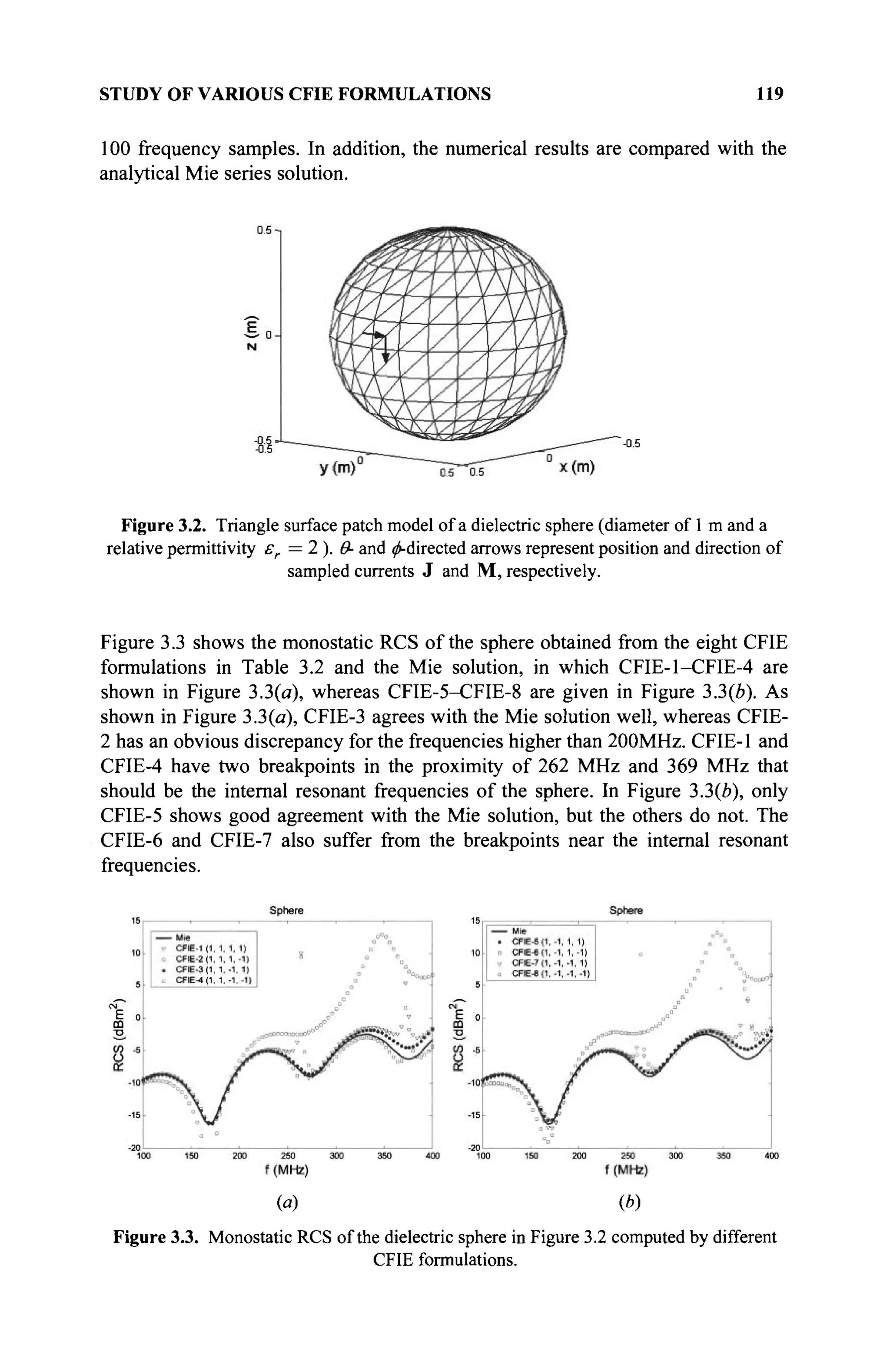
![120 ANALYSIS OF DIELECTRIC OBJECTS IN THE FREQ DOMAIN
The discrepancy between the CFIE solutions and the Mie series solution in the
studied frequency range can be evaluated by defining an averaged difference of
the monostatic RCS as
Ασ =
M
Σ 'Mie numerical IM (3.63)
where σ denotes the RCS. M is the number of samples in the whole frequency
range, and it is equal to 100 in this example. These average differences Δσ for
the eight CFIE formulations are given also in Table 3.2. CFIE-3 and CFIE-5 have
the lowest errors as 0.40 and 0.41, respectively, which is much lower than all the
others.
In the previous CFIE formulation, it is termed TENE-THNH, as there are
four terms to form the CFIE (i.e., CFIE = EFIE + n x EFIE + MFIE + n x MFIE
with fm as the testing functions or CFIE = EFIE + MFIE with fm + gm as the
testing functions). One suggestion from [6] is to drop one of these four terms and
thus the CFIE formulations can further be extended to TENE-TH, TENE-NH, TE-
THNH, or NE-THNH, depending on which term is neglected. For example, by
setting gH to zero, the testing of the magnetic field contains only the tangential
function fm and thus is referred to as TENE-TH. Applying this scheme to the
eight different CFIE formulations of Table 3.2 results in 16 possible formulations
for the CFIE with different testing coefficients, which are listed in Table 3.3.
TABLE 3.3. CFIE Formulations with Different Combinations of Testing Coefficients
and the Averaged Difference of Far Field and Monostatic RCS between the Mie Series
and the CFIE Solution for the Dielectric Sphere depicted in Figure 3.2
Formulation
TENE-TH
TENE-NH
TE-THNH
NE-THNH
(1)
(2)
(3)
(4)
(1)
(2)
(3)
(4)
0)
(2)
(3)
(4)
(1)
(2)
(3)
(4)
fE
+1
+1
+1
+1
+1
+1
+1
+1
+1
+1
+1
+1
0
0
0
0
Testing coefficients
gE
+1
+1
-1
-1
+1
+1
-1
-1
0
0
0
0
+1
+1
+ 1
+1
fn
+1
-1
+1
-1
0
0
0
0
+1
+1
-1
-1
+1
+1
-1
-1
gH
0
0
0
0
+1
-1
+1
-1
+1
-1
+1
-1
+1
-1
+1
-1
Aee
(mV)
12.0
4.1
4.7
4.5
3.5
7.8
2.4
8.2
9.4
8.1
8.7
6.9
5.1
5.7
5.7
5.3
Ьеф
(mV)
16.7
6.4
6.0
24.0
12.9
32.1
20.3
21.4
5.5
9.8
7.2
16.4
12.9
16.4
21.5
15.6
Δσ
(dBm2
)
0.79
0.30
0.34
0.51
0.28
0.22
0.37
0.48
0.61
0.59
0.55
0.49
0.42
0.48
0.52
0.45](https://image.slidesharecdn.com/timeandfrequencydomainsolutionsofemproblemsusingintegralequationsandahybridmethodologyb-250205130750-568a5ba2/75/Time-and-Frequency-Domain-Solutions-of-EM-Problems-Using-Integral-Equations-and-a-Hybrid-Methodology-B-H-Jung-pdf-142-2048.jpg)
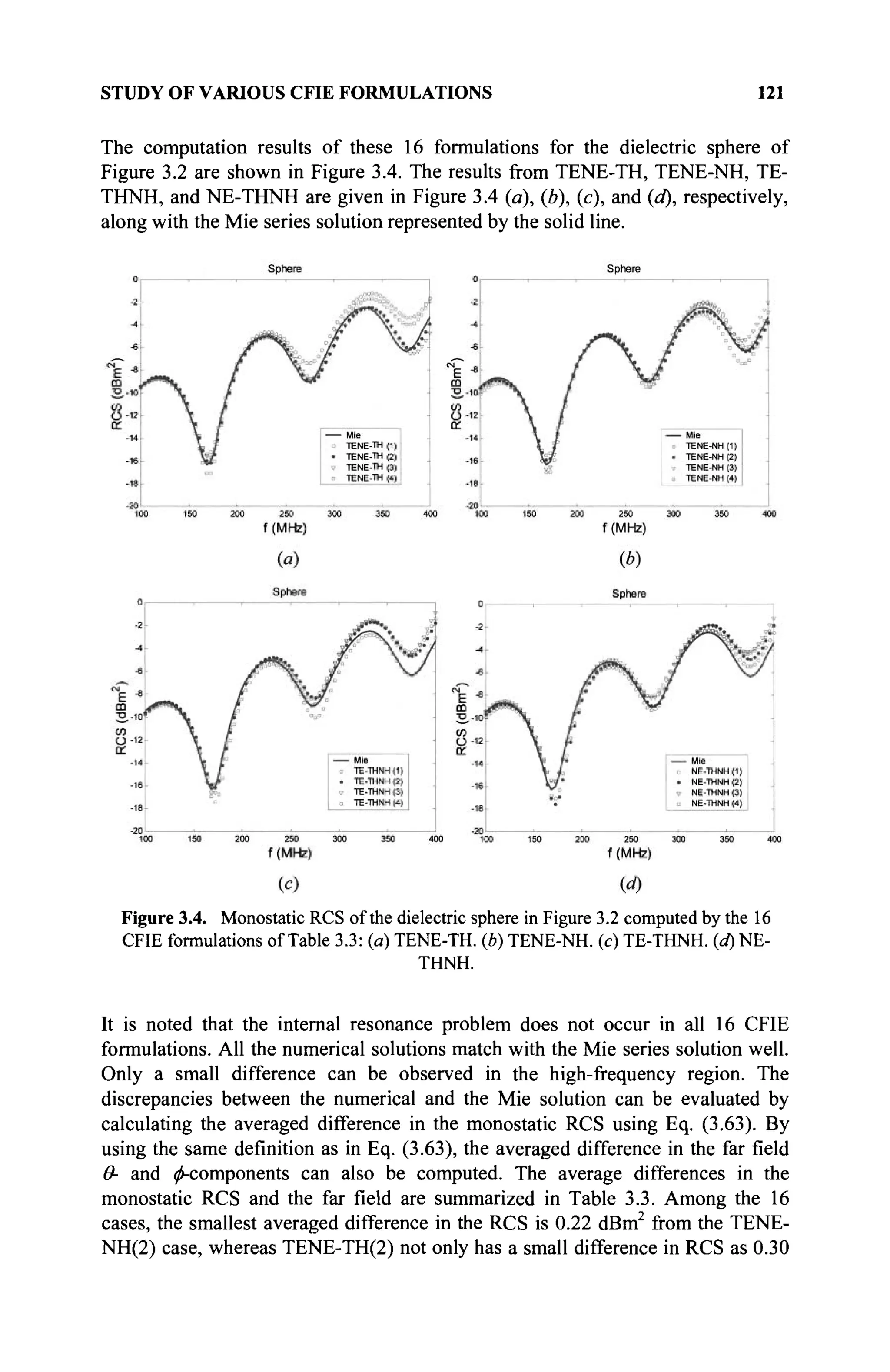
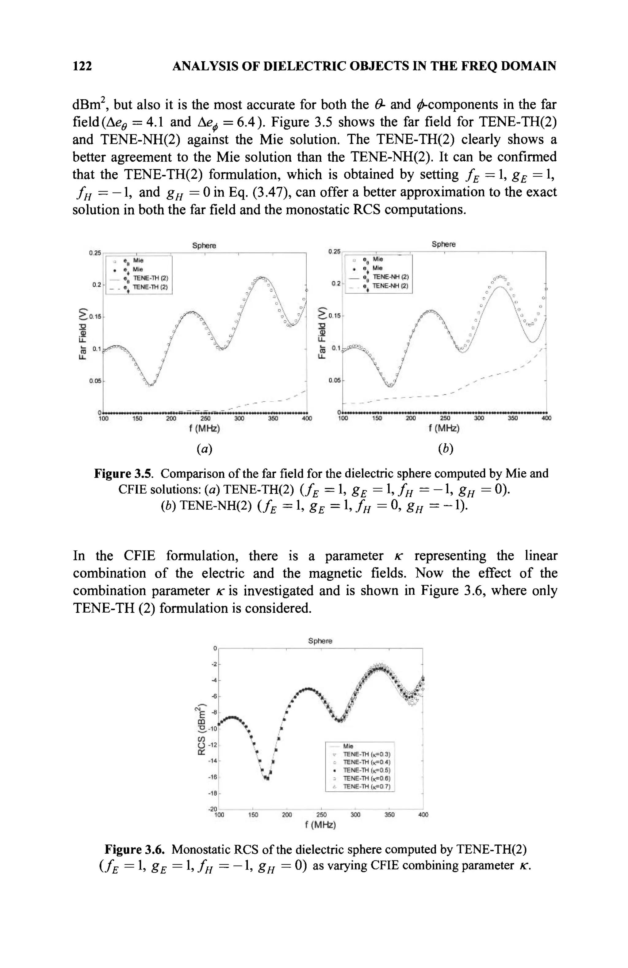
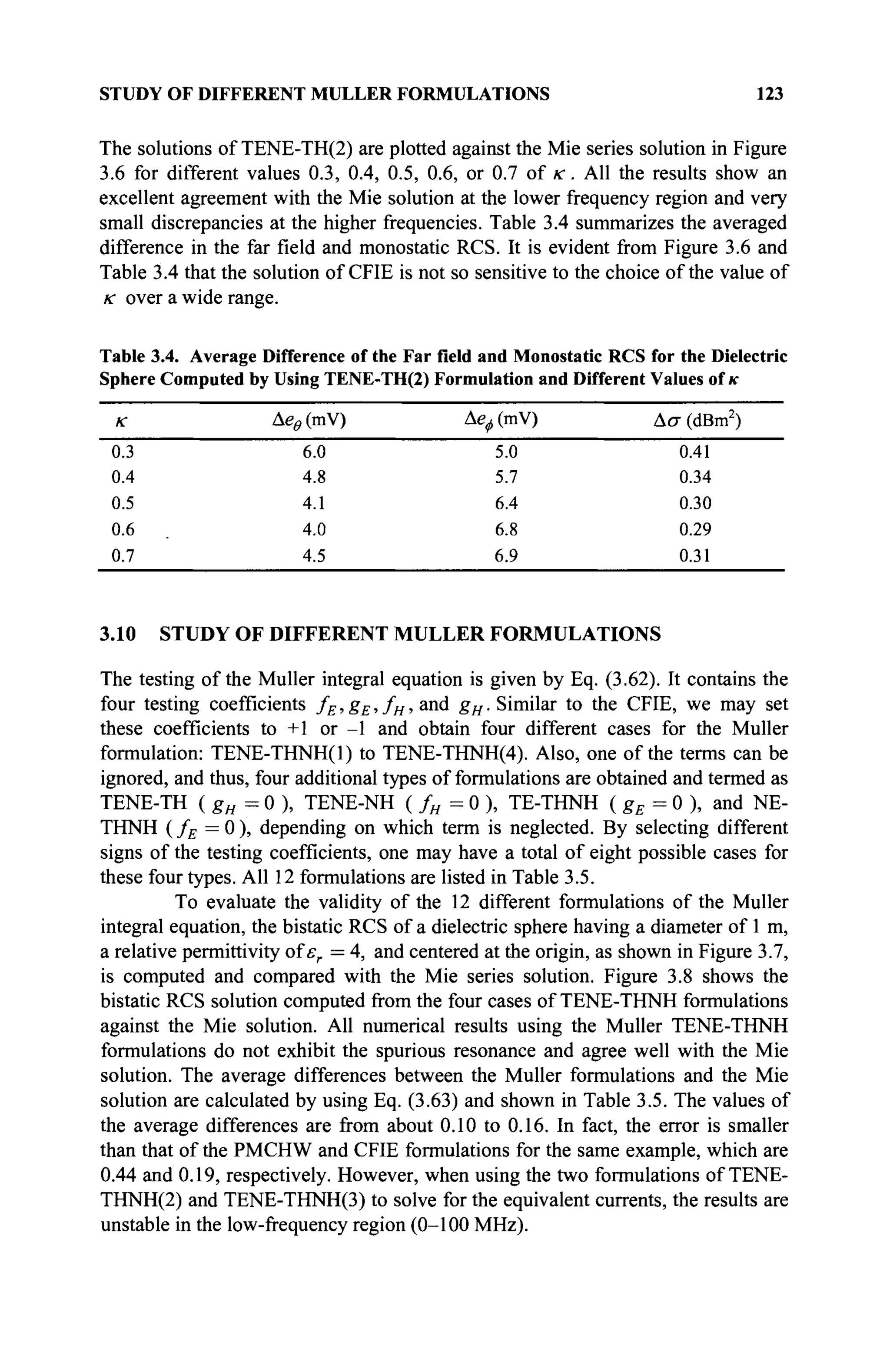
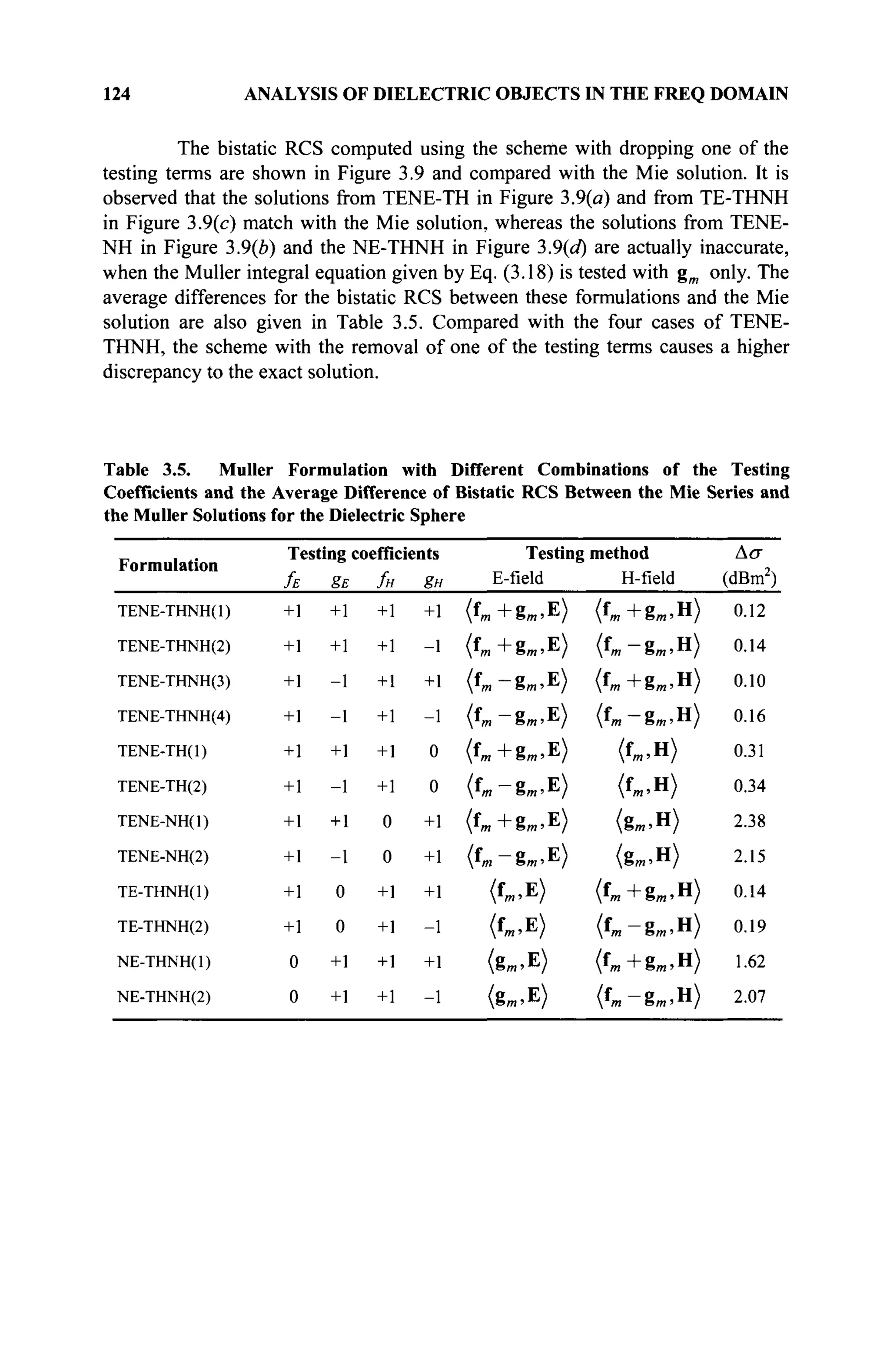
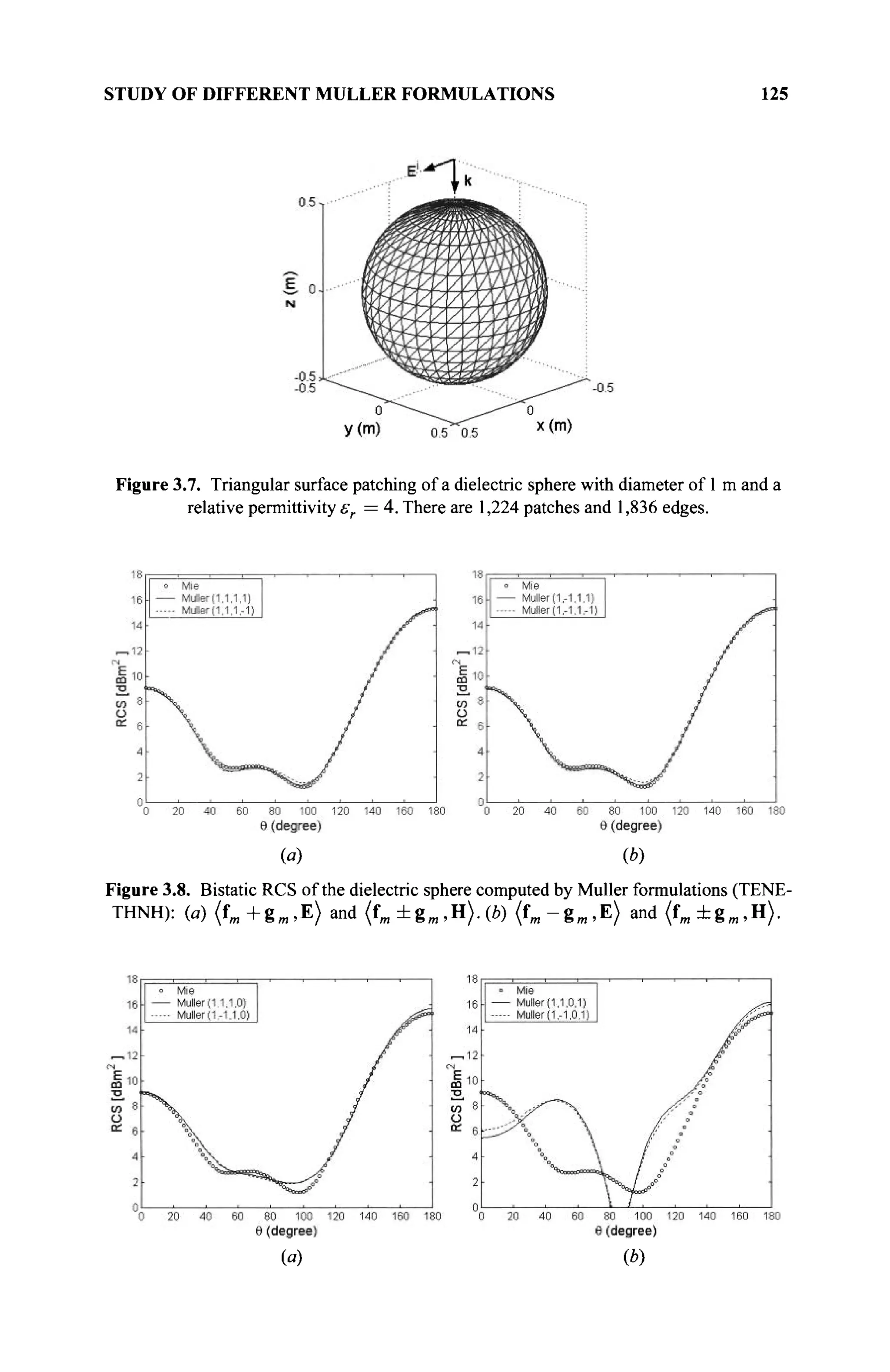
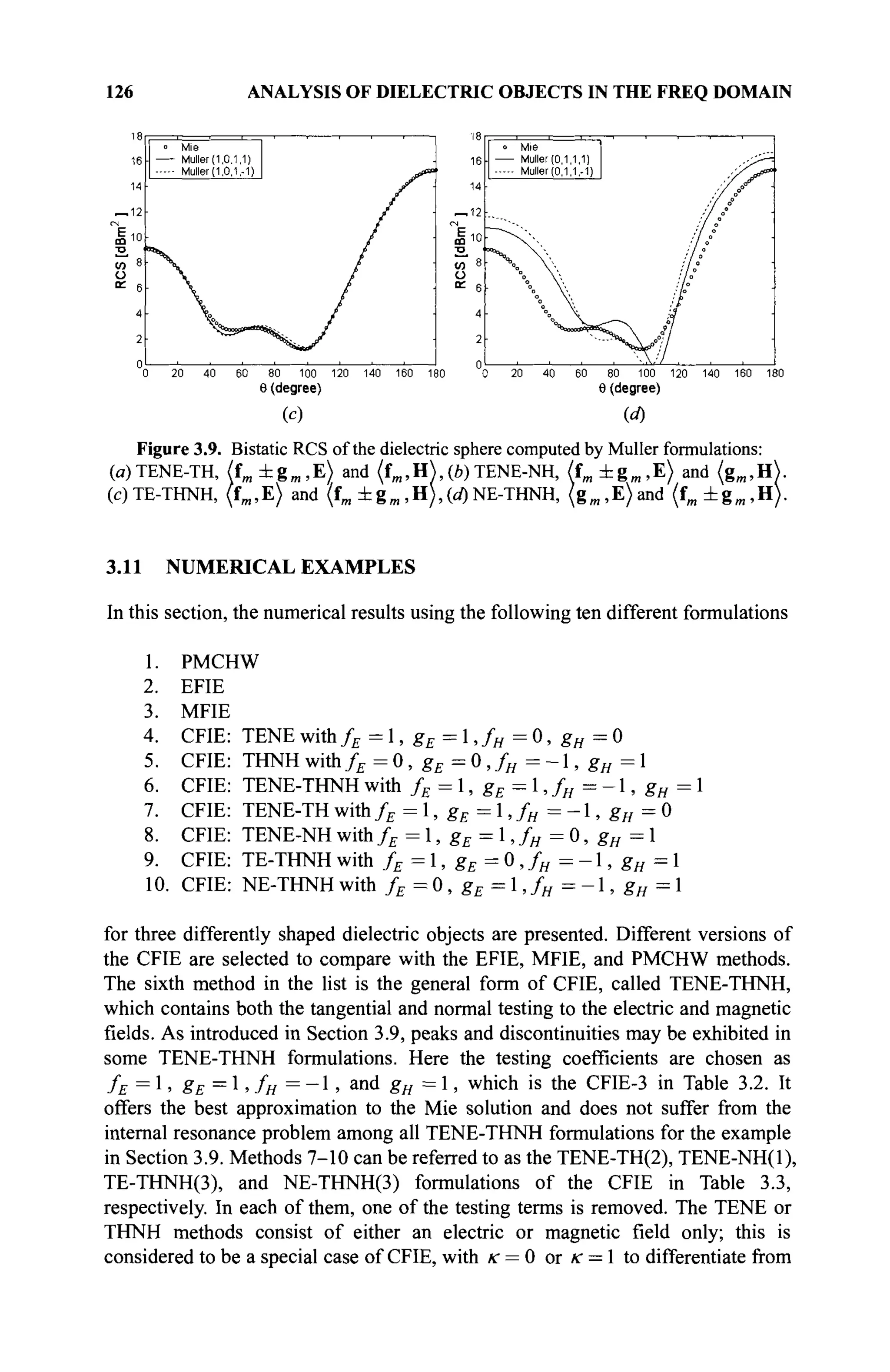
![NUMERICAL EXAMPLES 127
EFIE or MFIE as previously described in Sections 3.4 and 3.5. The value к = 0.5
is chosen for all CFIE formulations.
The object to be analyzed is a dielectric sphere, a cube, or a cylinder with
a relative permittivity er = 2. In the numerical calculation, the scatterers are
illuminated from the top by an incident x-polarized plane wave with a propagation
vector к = —z, as used in the previous section. The frequency range over which
the results are calculated is 0 < / < 400 MHz at an interval of 4 MHz. The
equivalent electric and magnetic currents, the far field, and the monostatic RCS
are computed. The equivalent currents computed by the PMCHW formulation are
used to compare with the results from the other formulations. In the analysis of the
sphere, the computed far fields and RCS are compared with the analytical Mie
series solution. Because the analytical solution of the far field or the monostatic
RCS for a cube or cylinder are not known, the commercially available higher order
basis-function-based integral equation solver (HOBBIES) [11] solution is used
instead. Both the Mie and HOBBIES solutions are calculated at the same
frequency interval of 4 MHz.
3.11.1 Dielectric Sphere
The first example is the dielectric sphere as shown in Figure 3.2. The ^-directed
electric current and the ^-directed magnetic current, as indicated by arrows in
Figure 3.2, are observed.
3.11.1.1 Analysis of a Sphere by PMCHW. Figure 3.10 shows the computed far
field and monostatic RCS using the PMCHW formulation. The far field and RCS
agree well with the Mie solution except for a small difference in the high-
frequency region. The currents are used to compare with other numerical results
and thus will be shown later.
liirtT i i i m r I -30 < < > > ^ ' > ' -'
0 50 100 150 200 250 300 350 400 0 50 100 150 200 250 300 350 400
f (MHz) f (MHz)
(a) (b)
Figure 3.10. PMCHW results for a dielectric sphere: (a) Farfield,(b) Monostatic RCS.](https://image.slidesharecdn.com/timeandfrequencydomainsolutionsofemproblemsusingintegralequationsandahybridmethodologyb-250205130750-568a5ba2/75/Time-and-Frequency-Domain-Solutions-of-EM-Problems-Using-Integral-Equations-and-a-Hybrid-Methodology-B-H-Jung-pdf-149-2048.jpg)
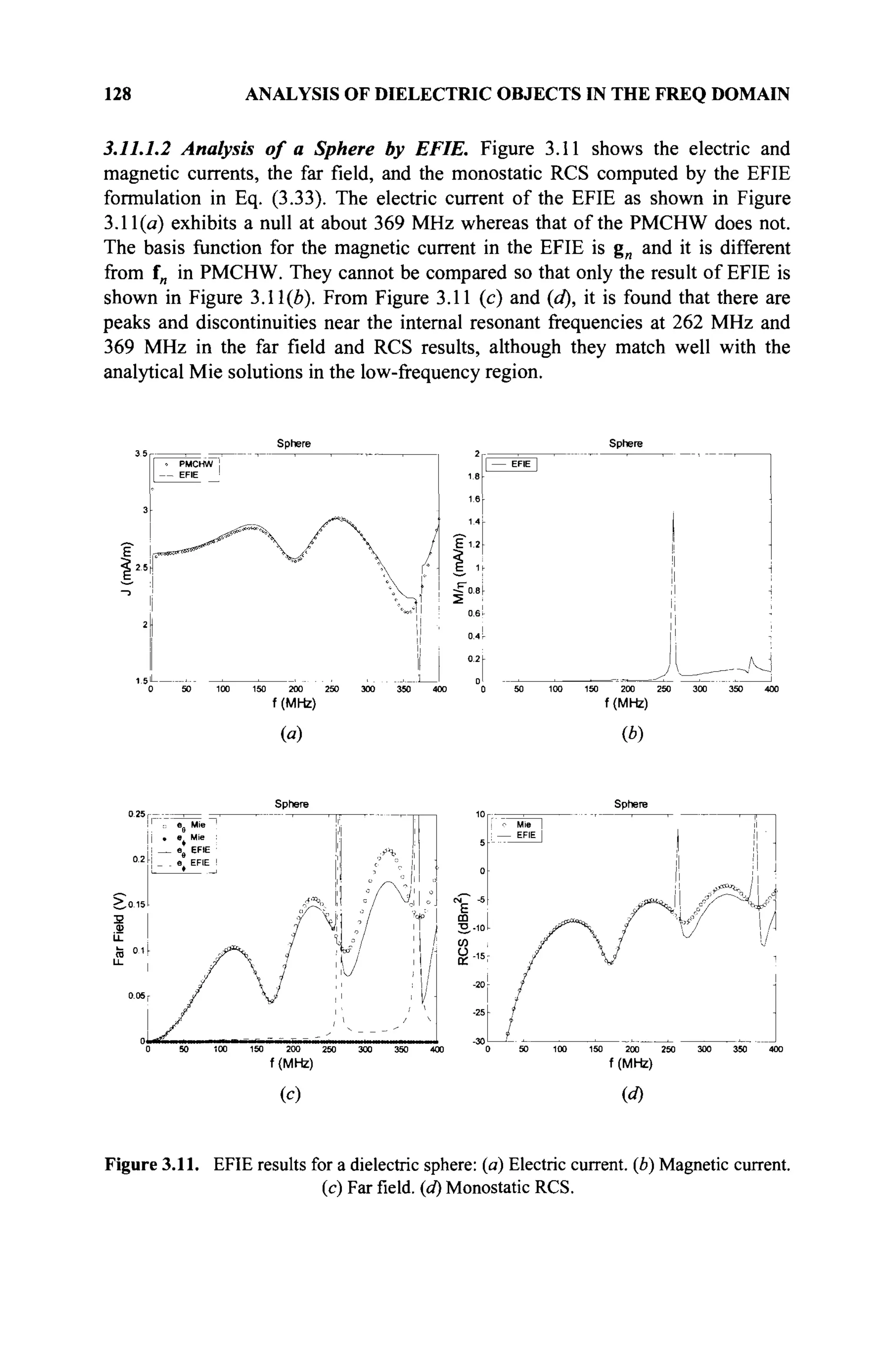
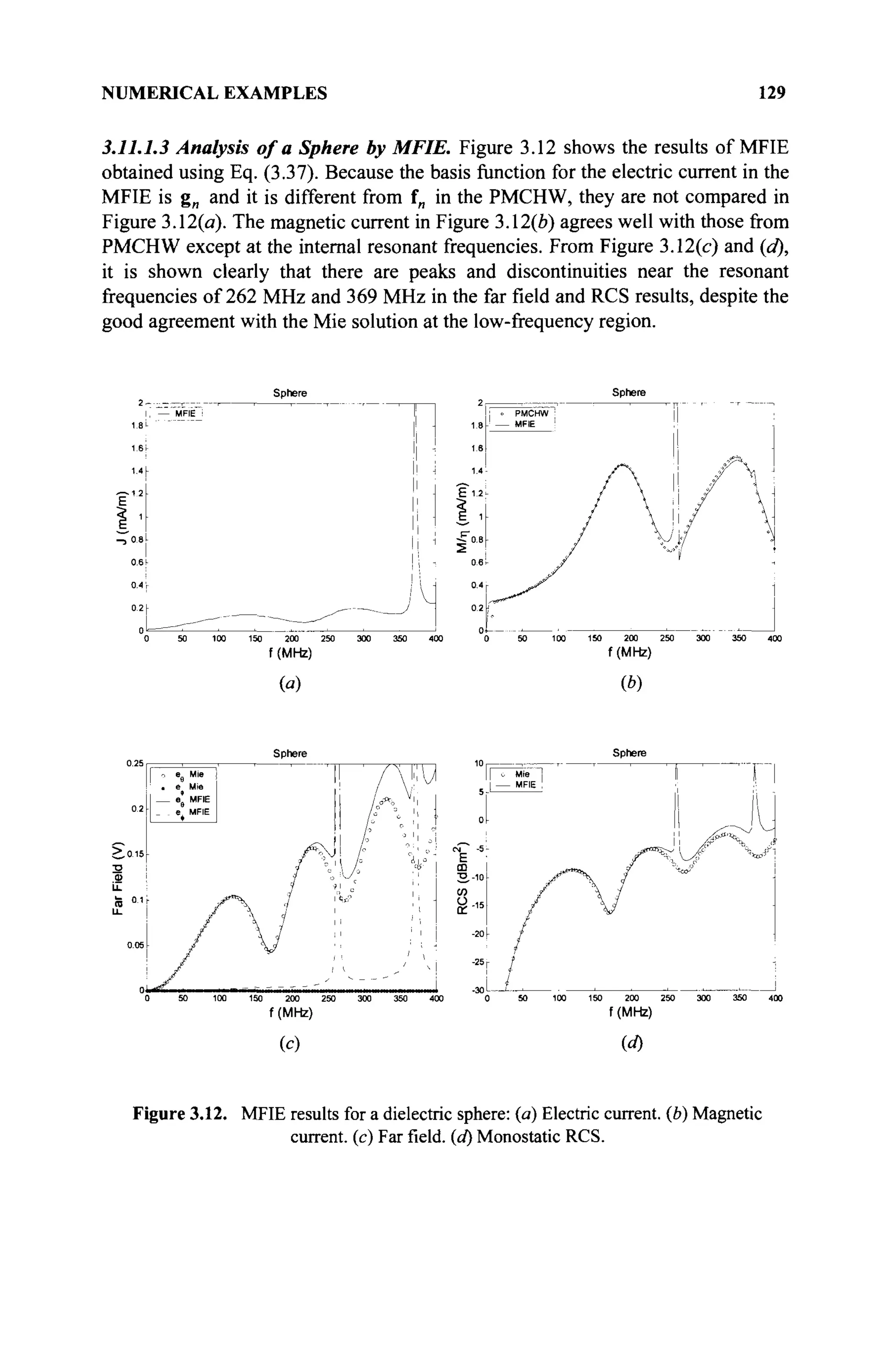
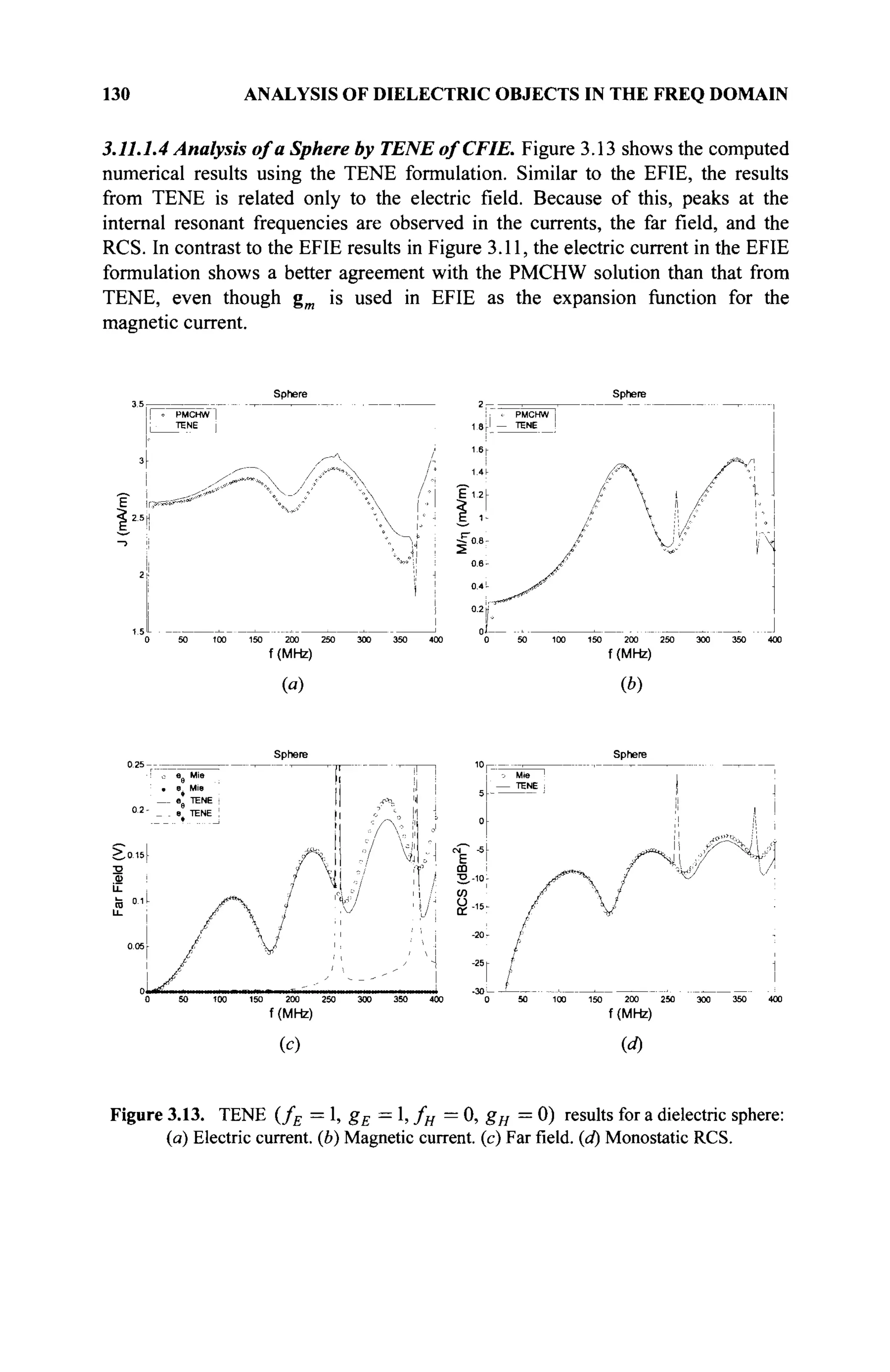
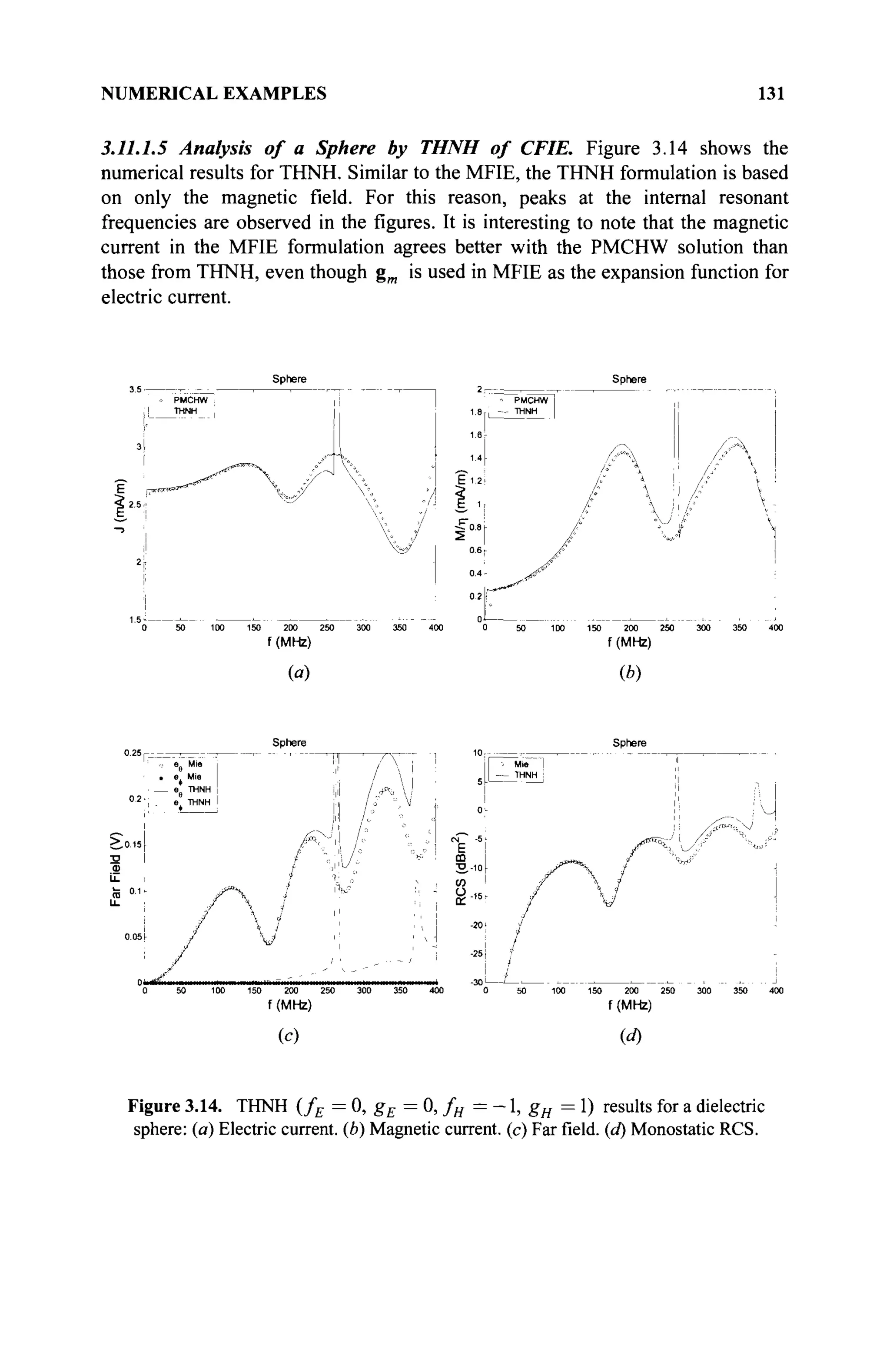
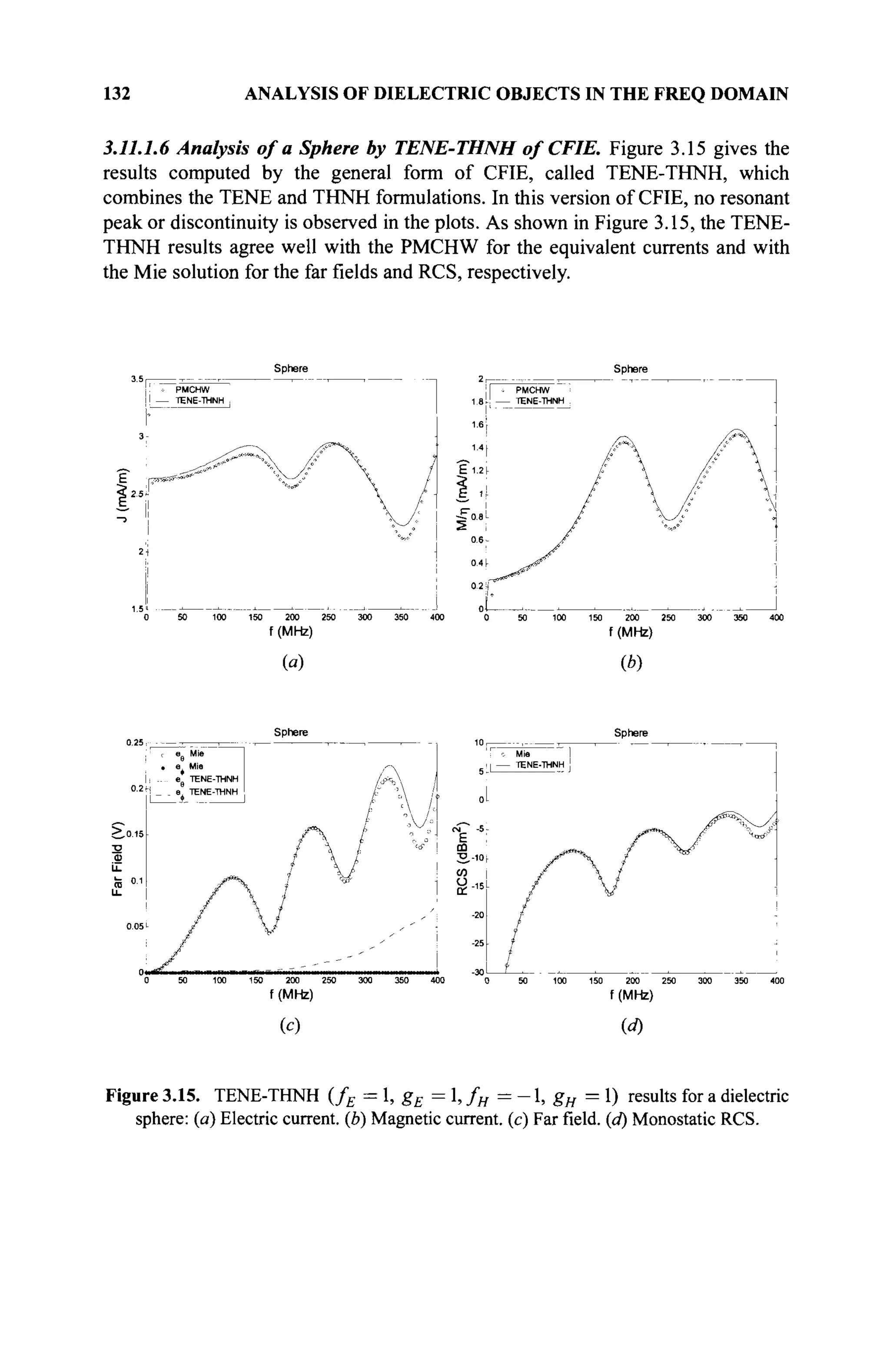

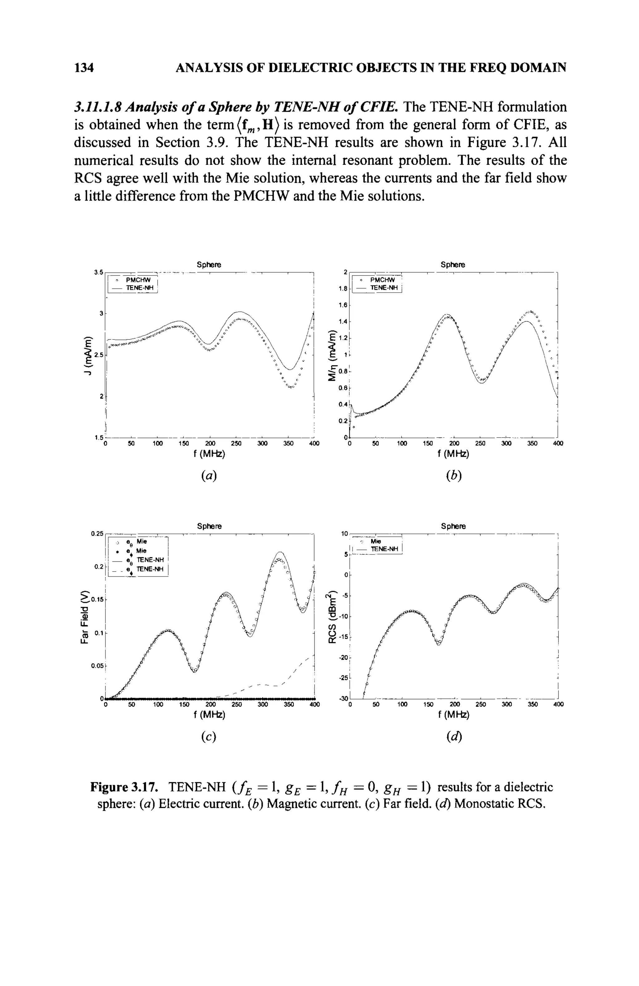
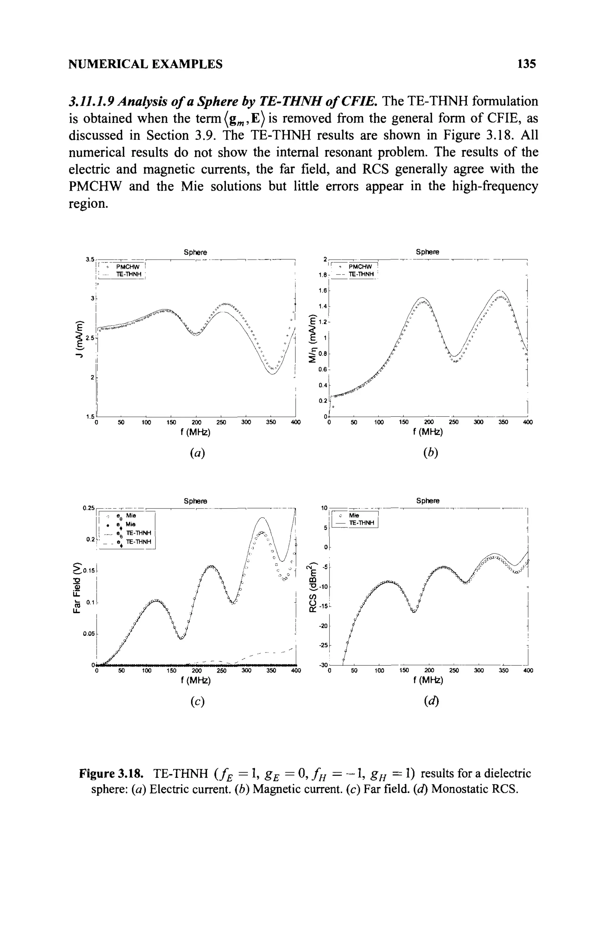
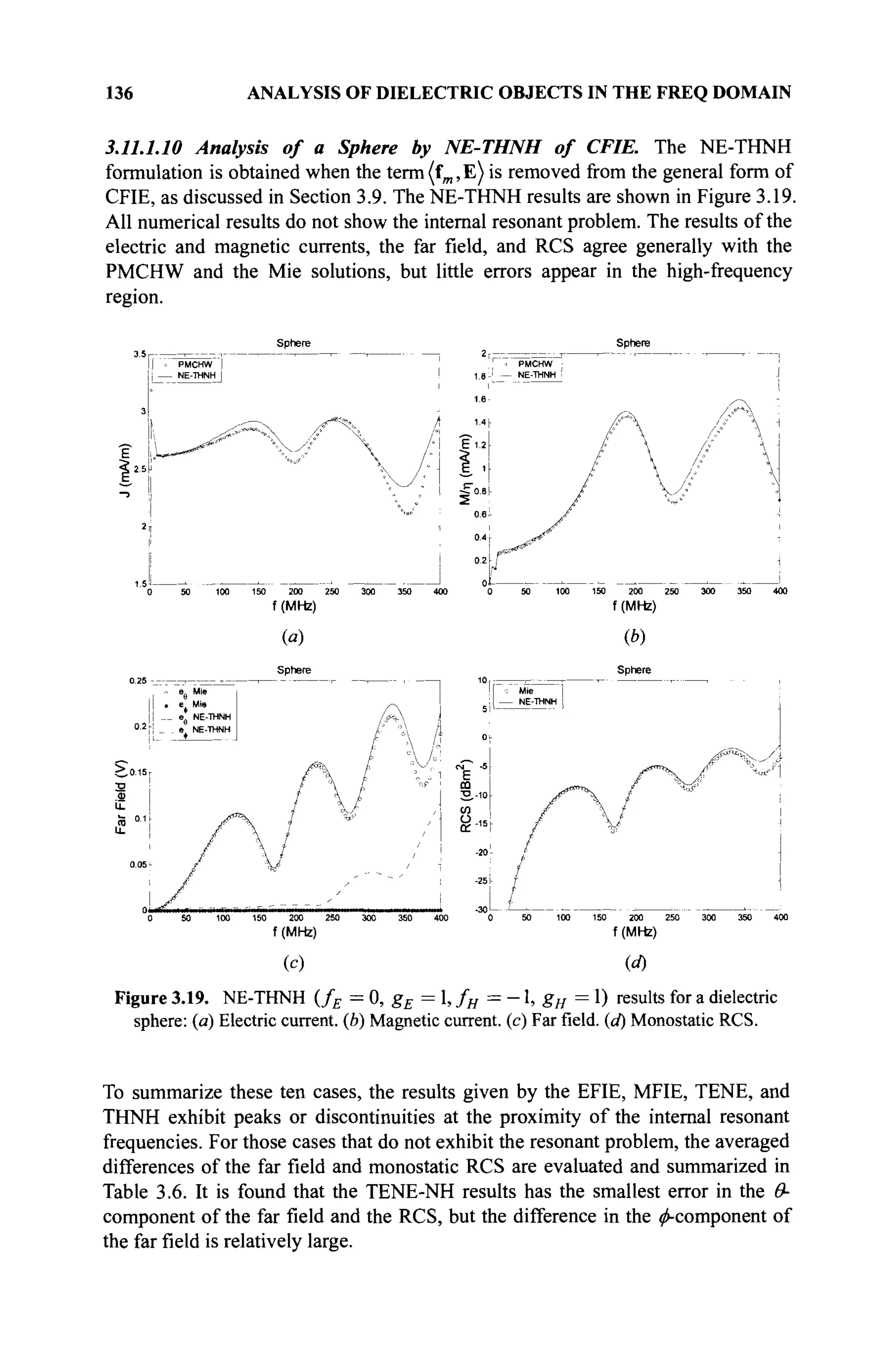
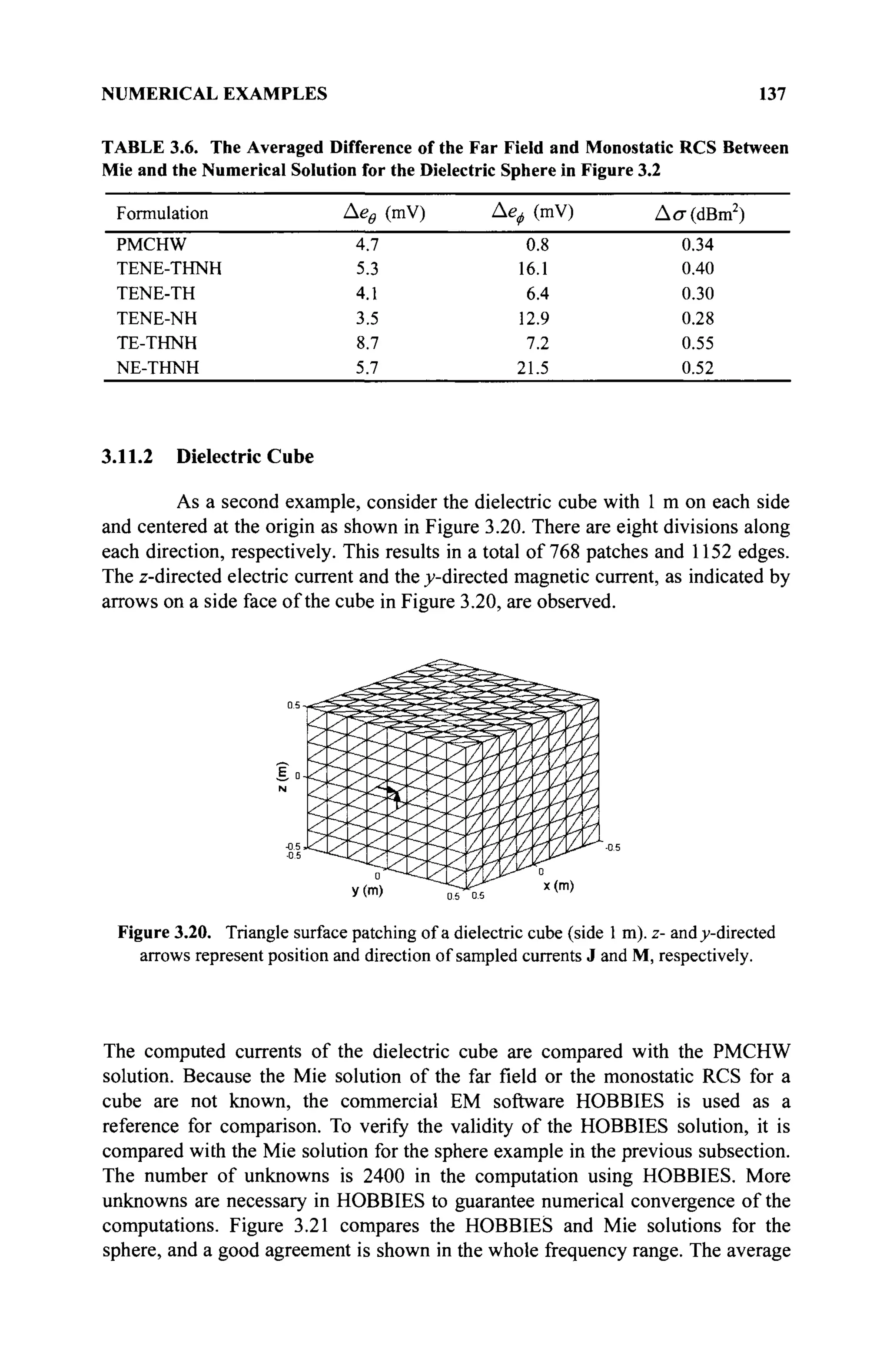
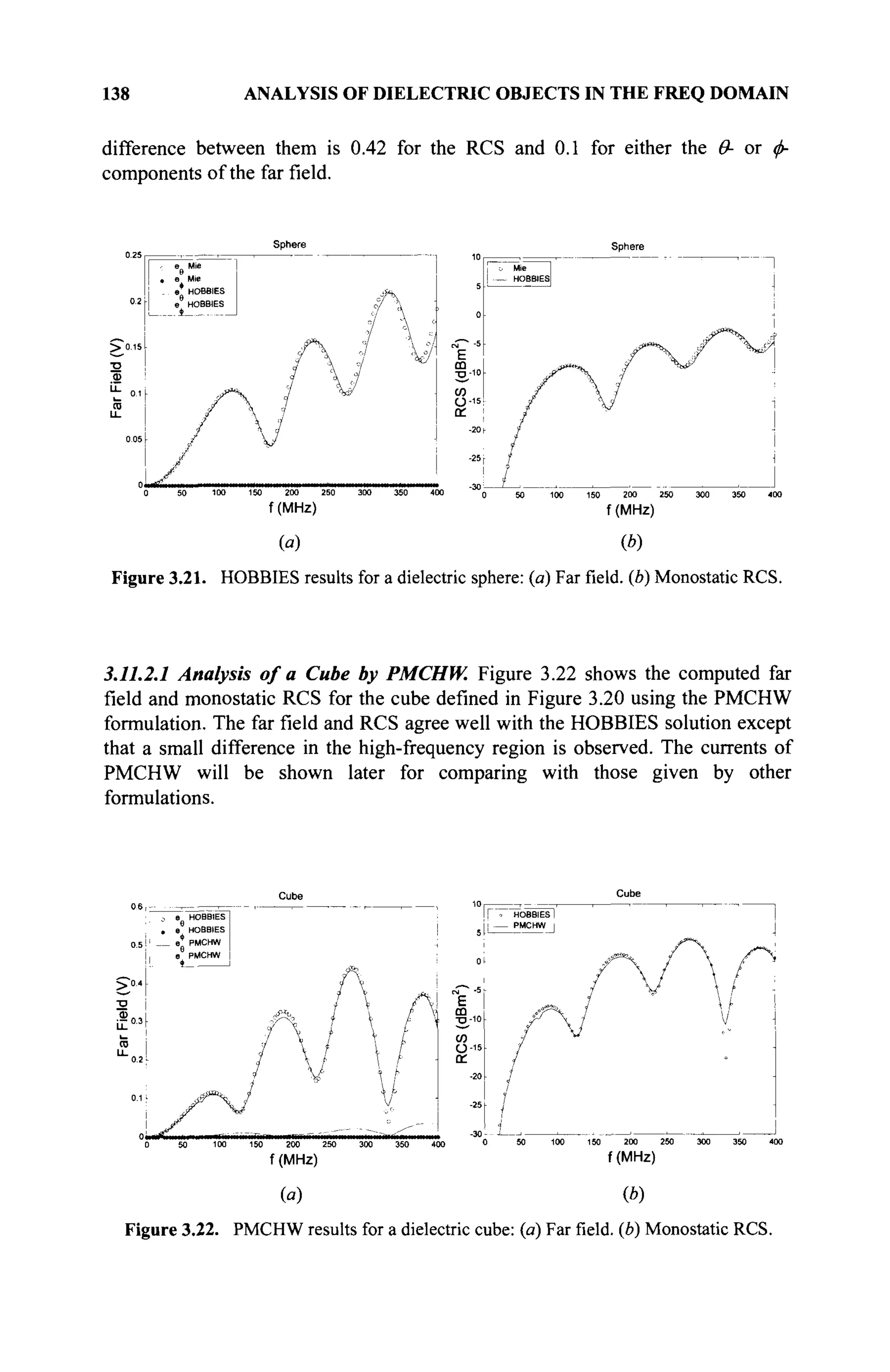
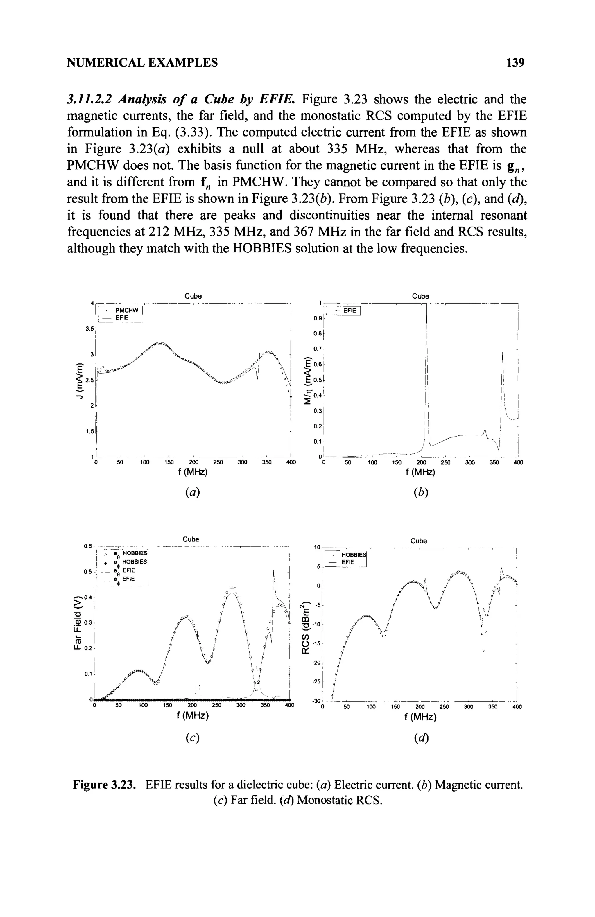
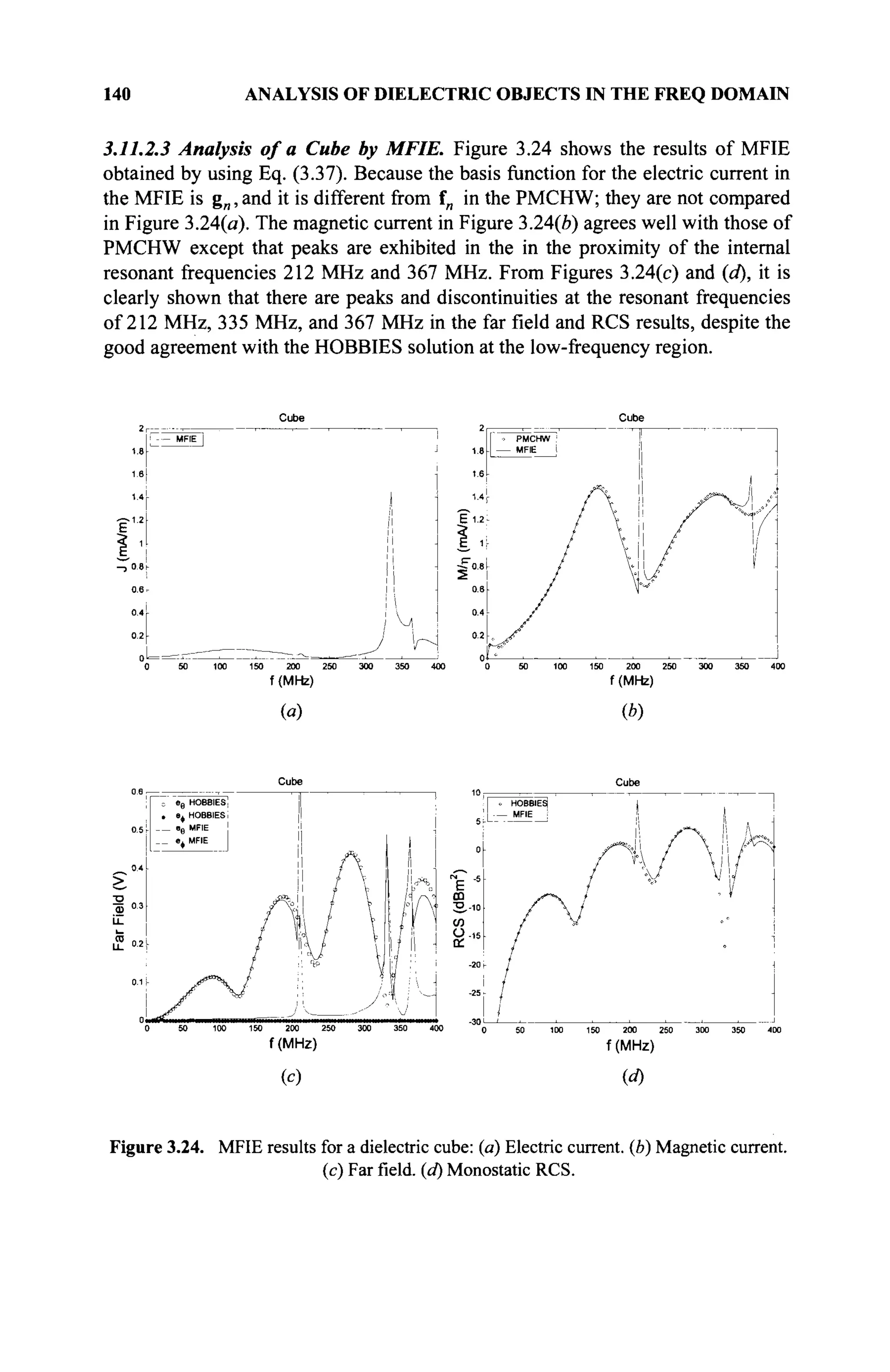
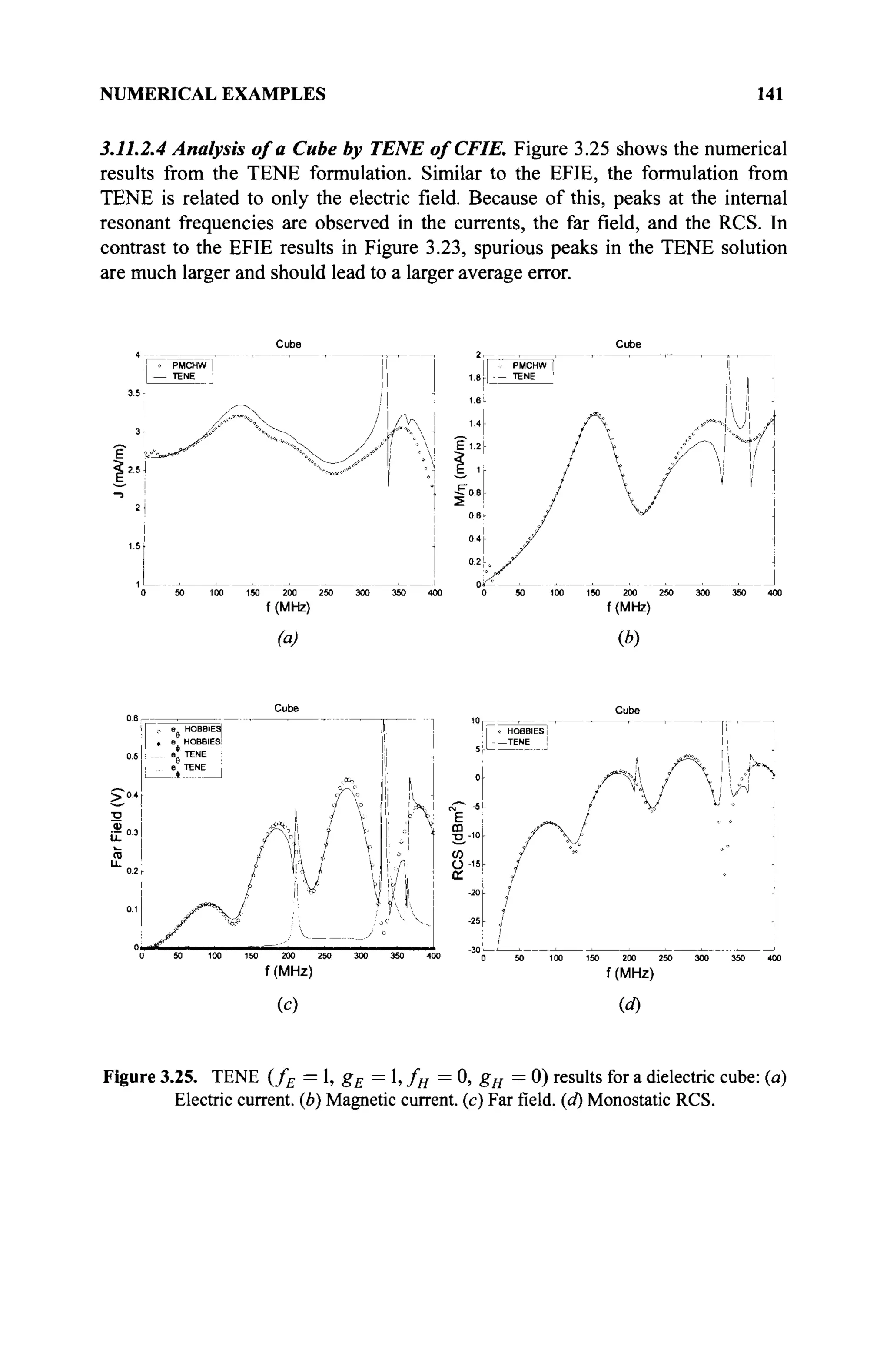
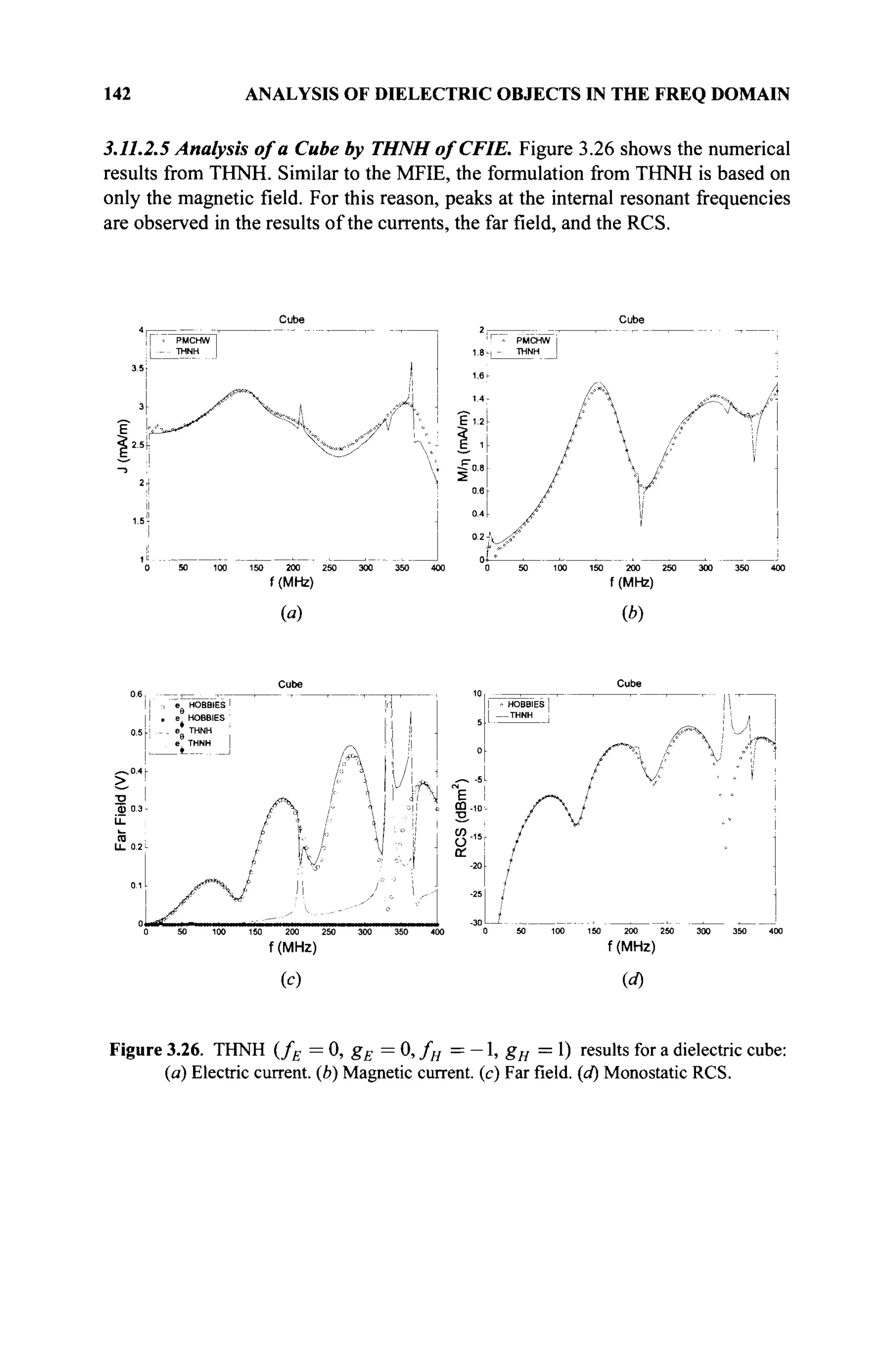

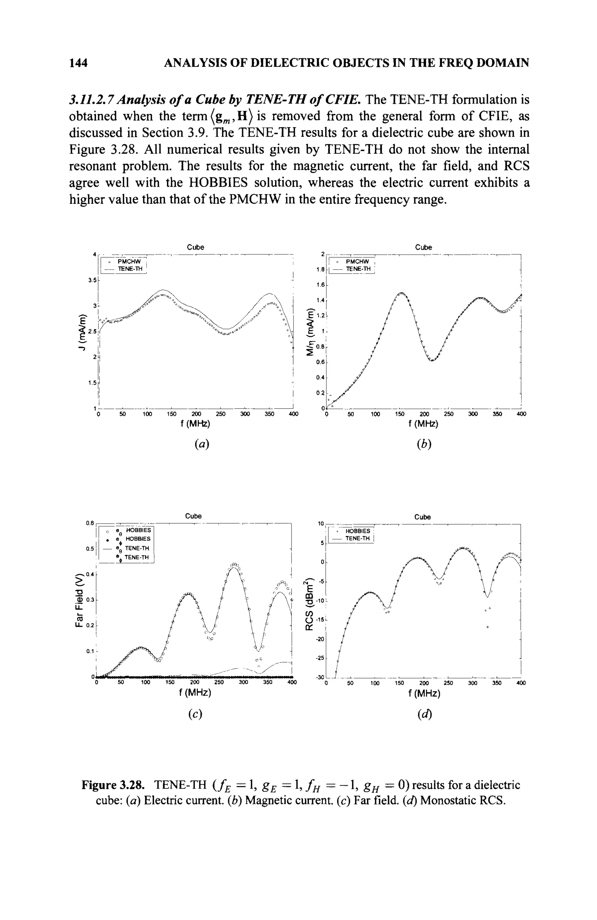
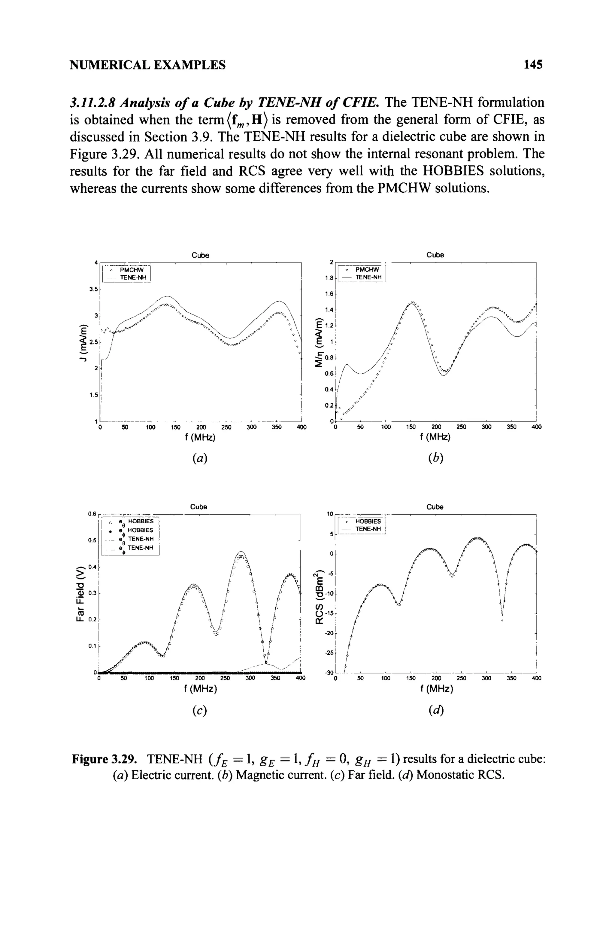
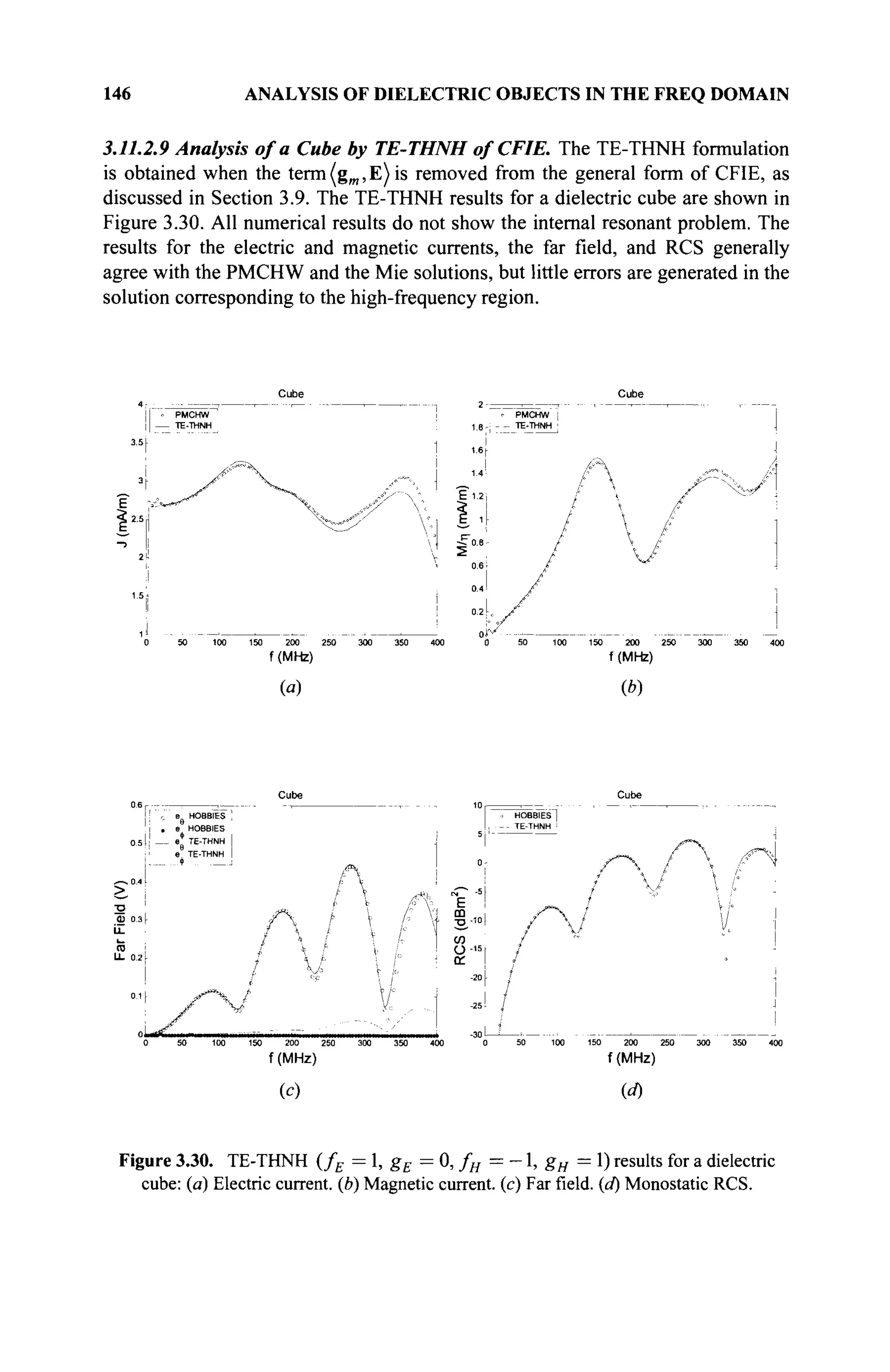
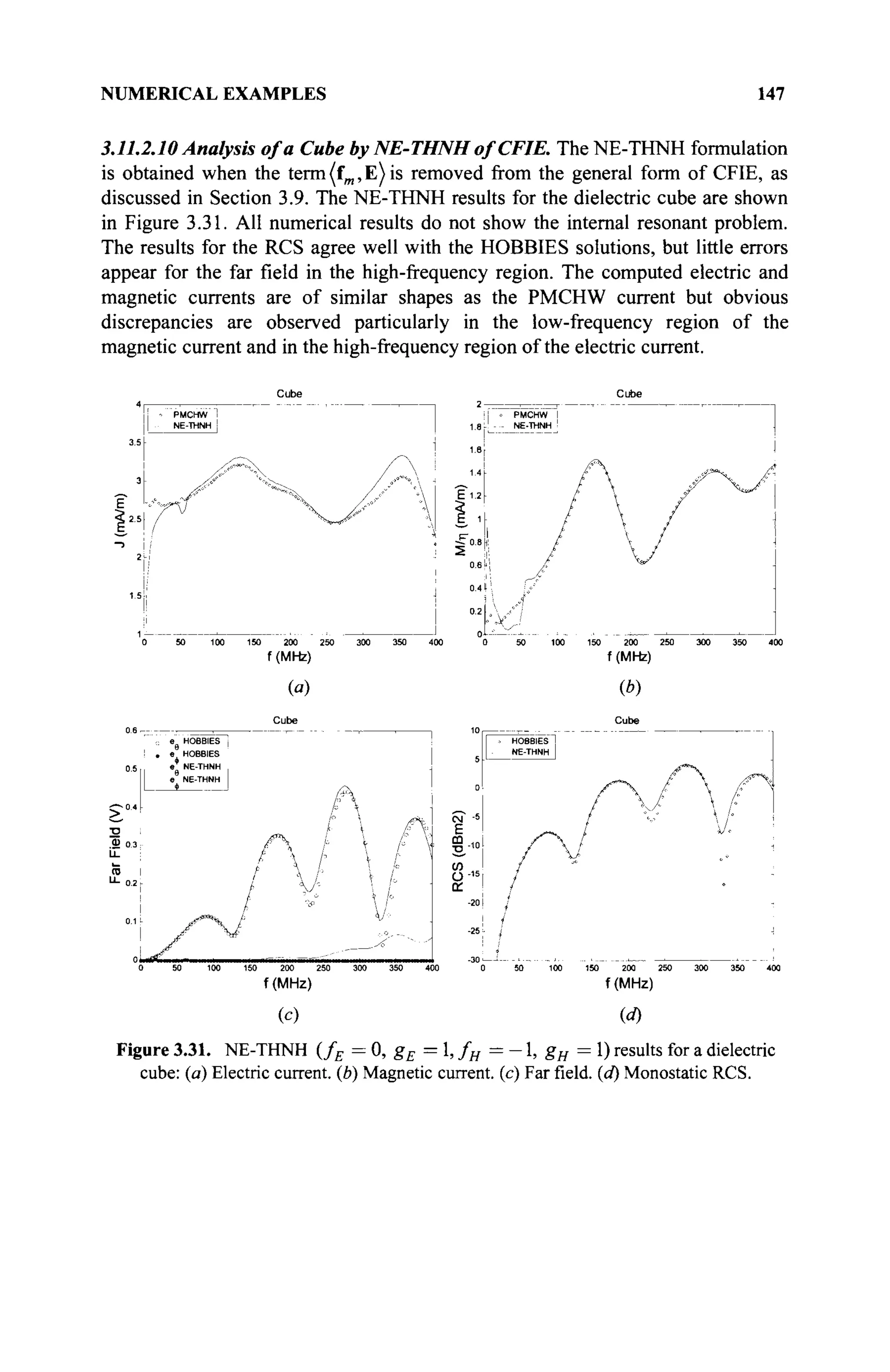
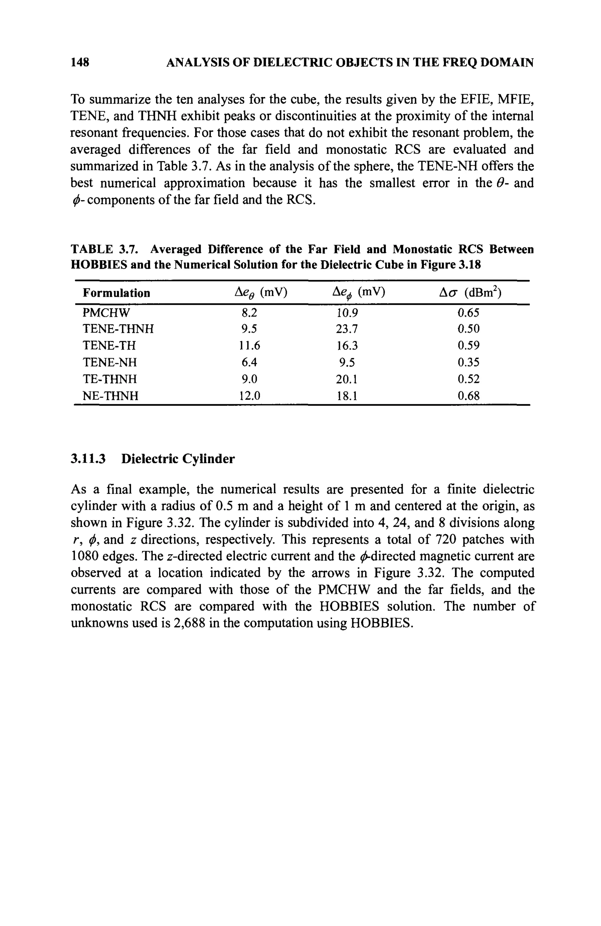
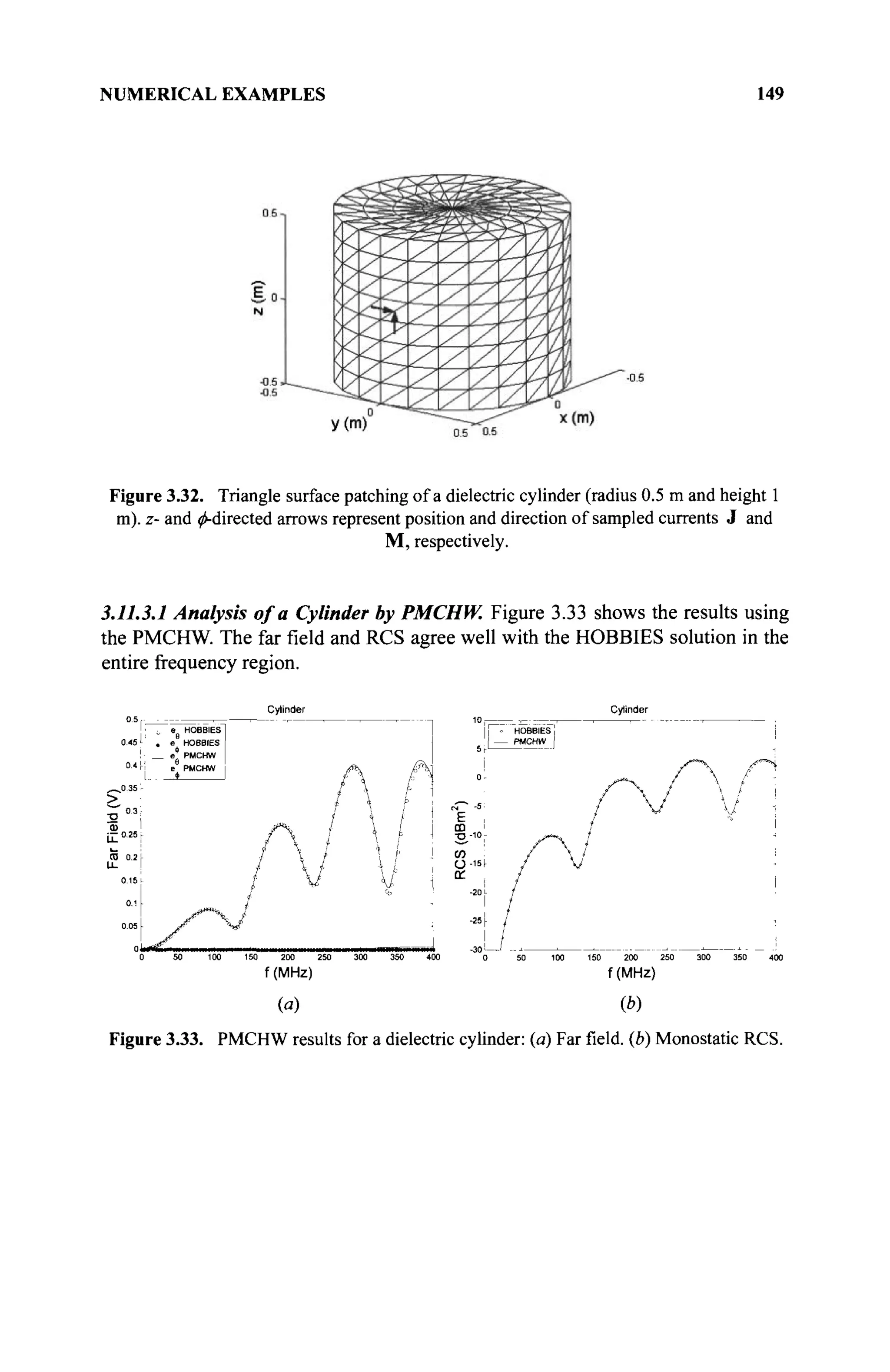
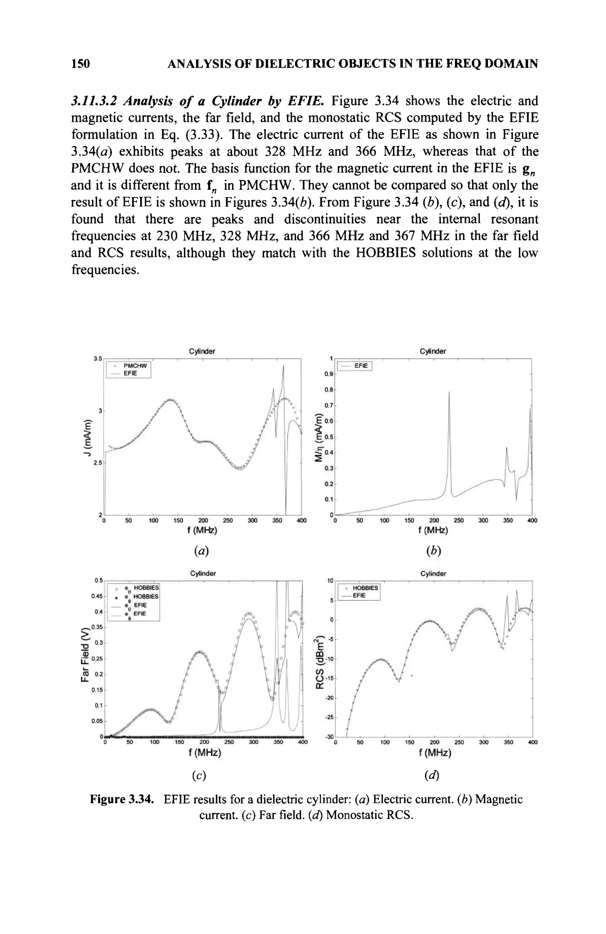
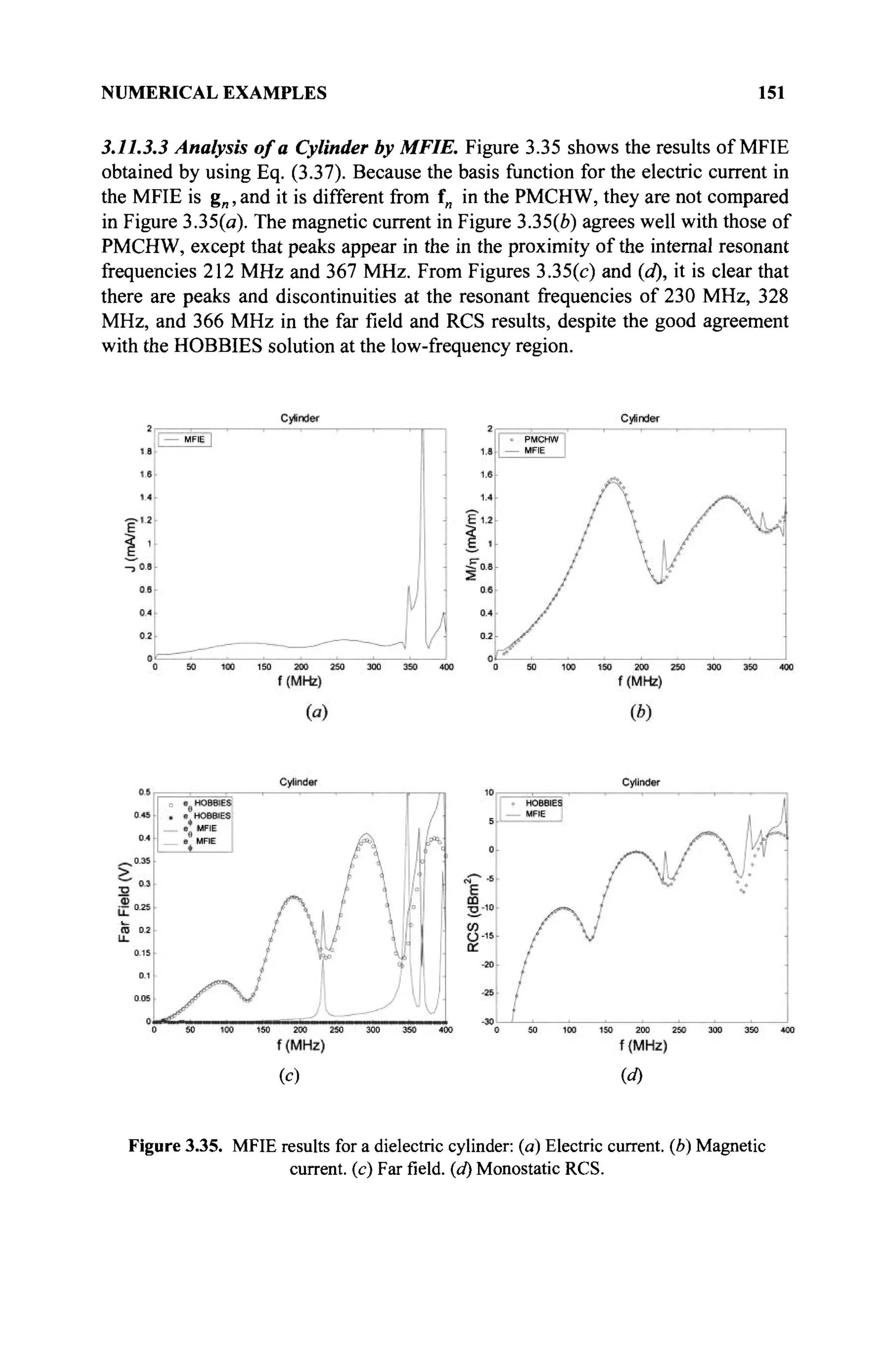
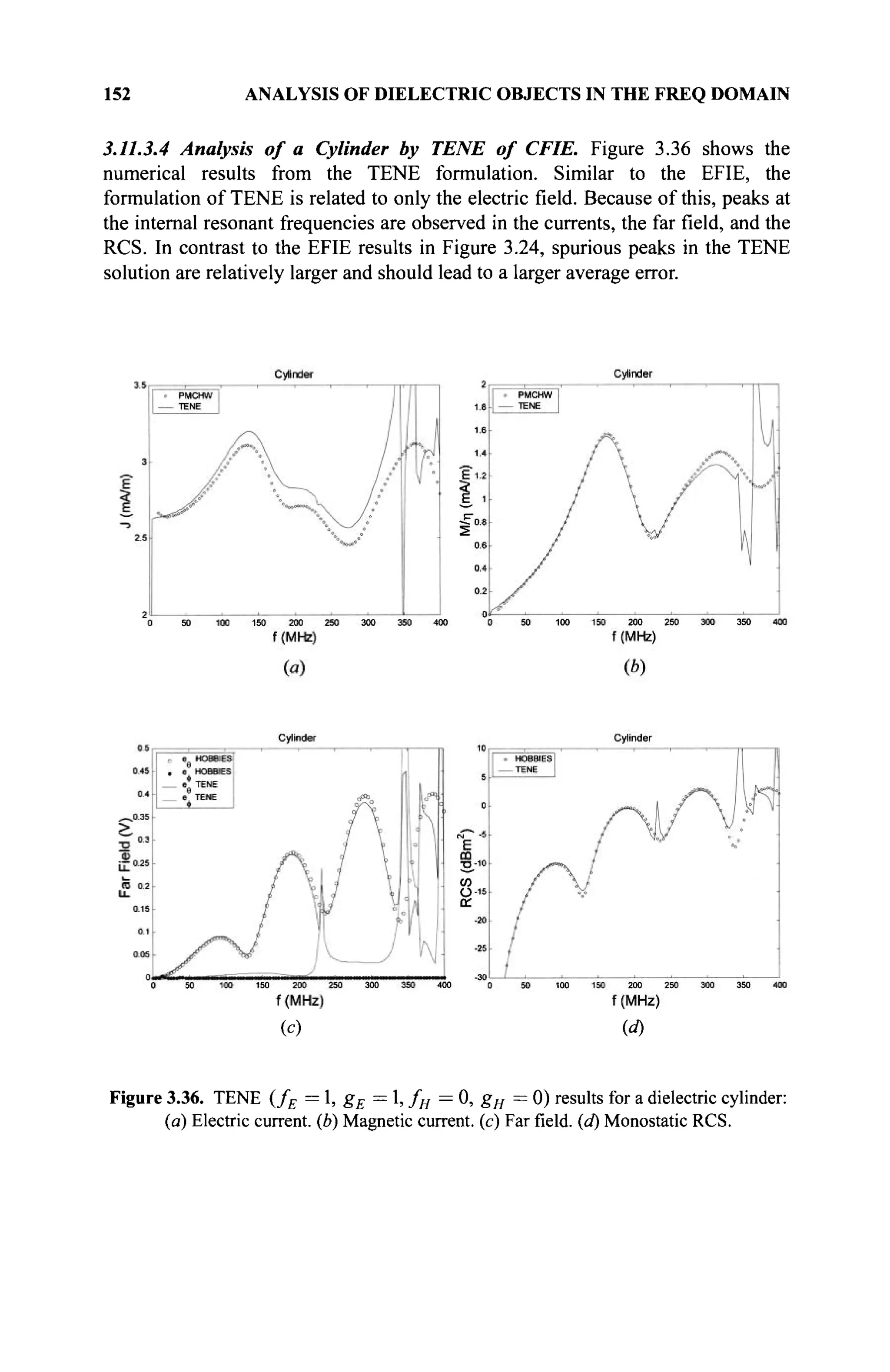
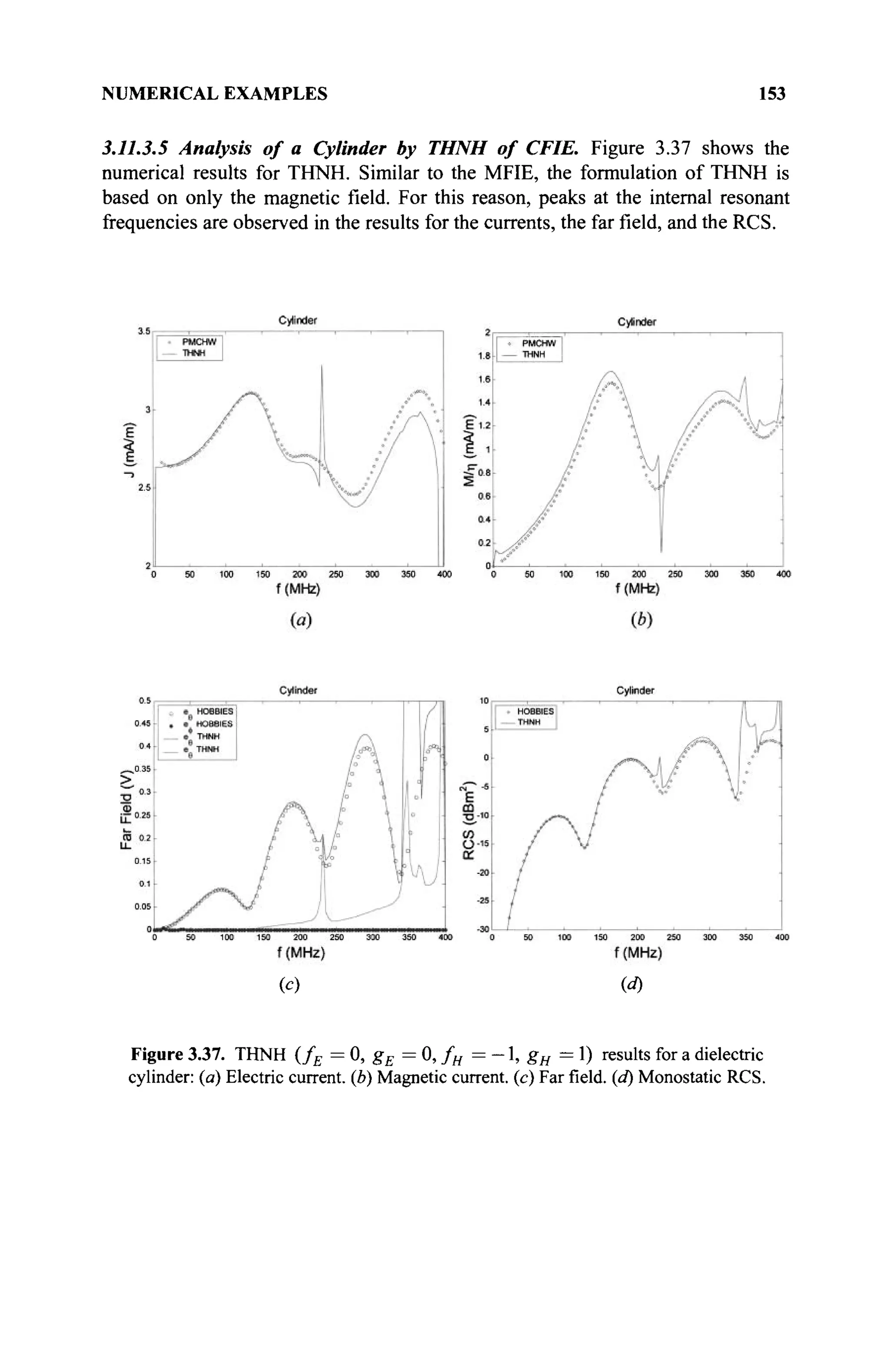
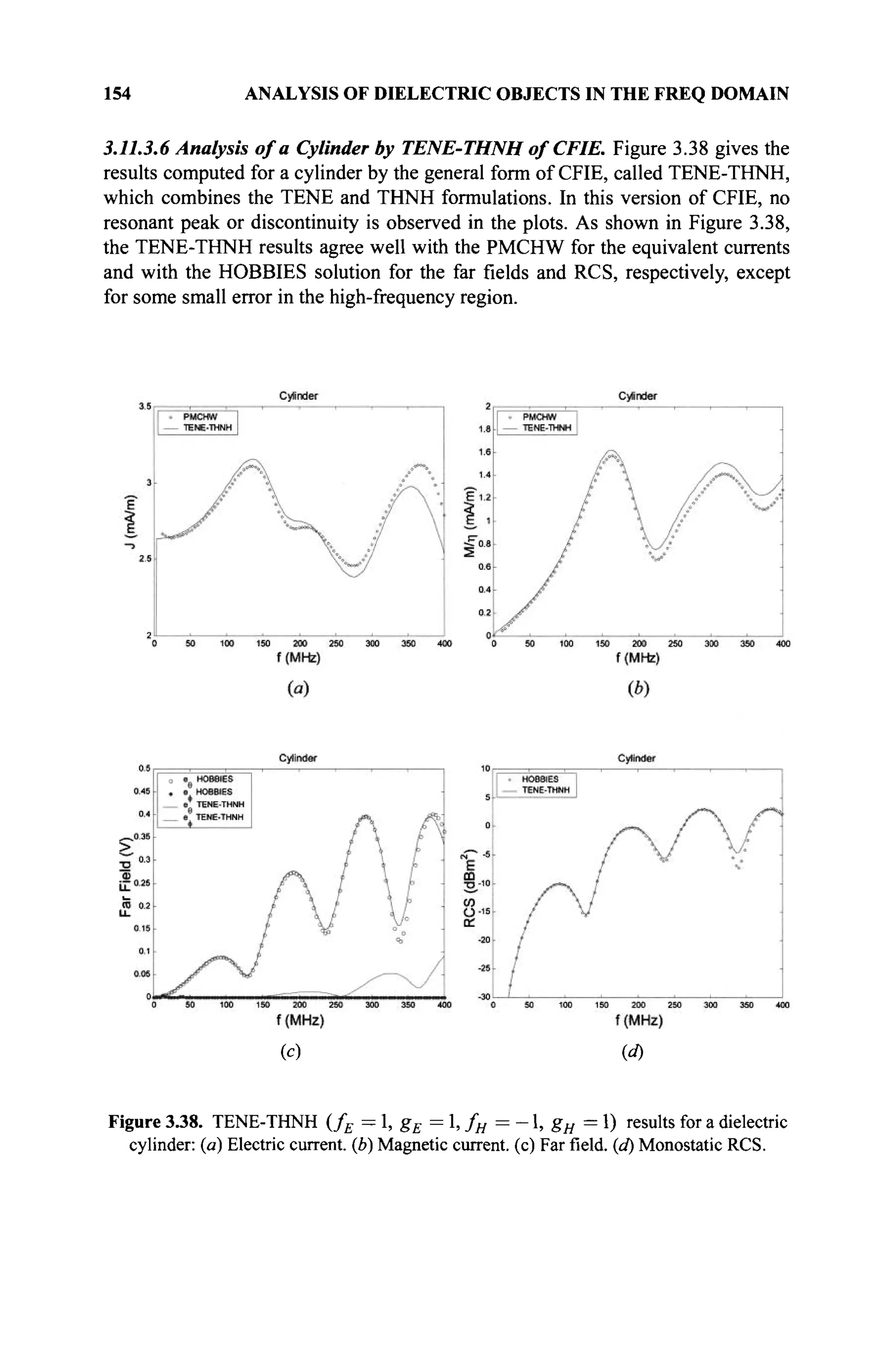
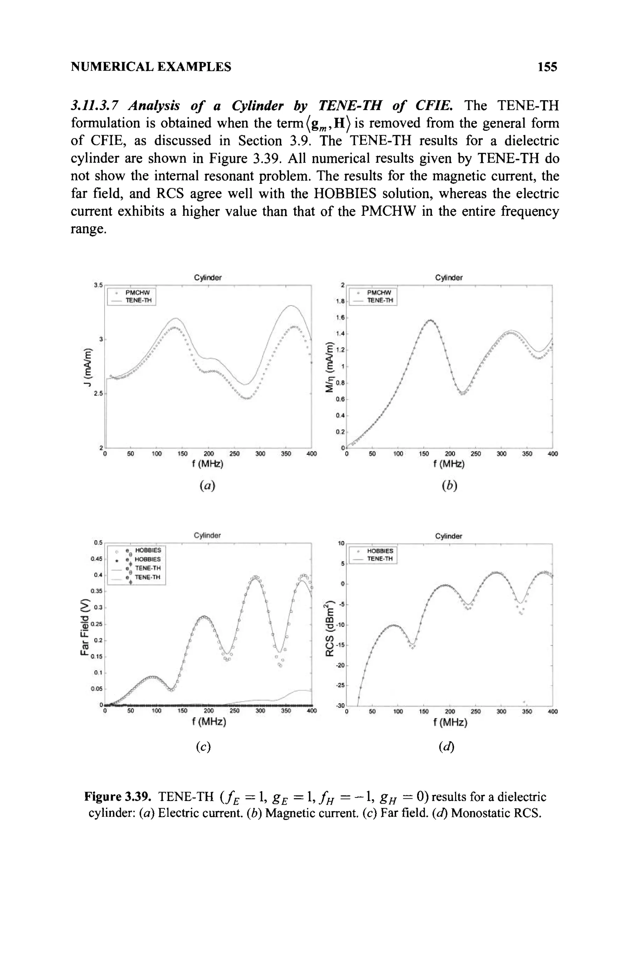
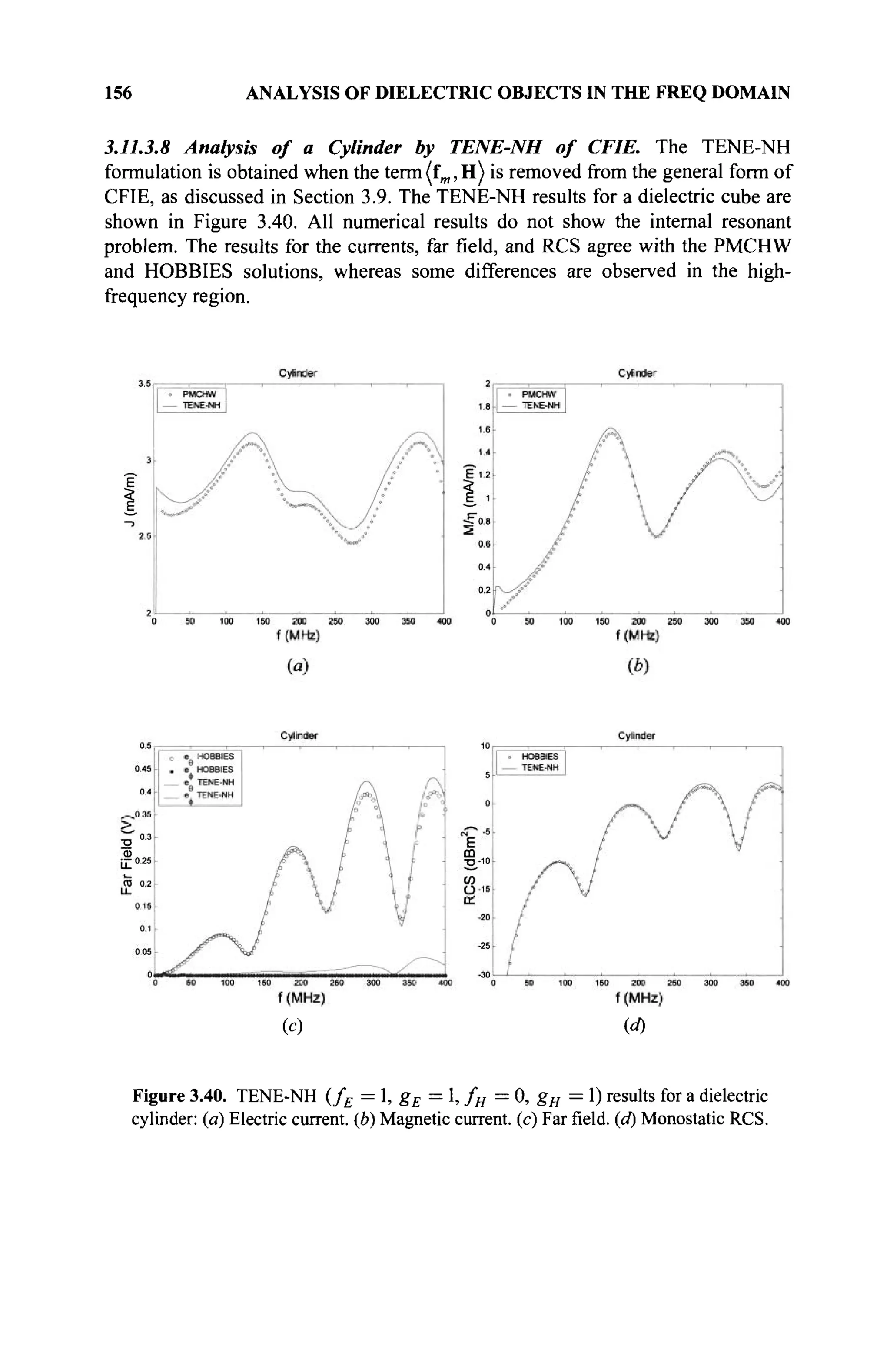
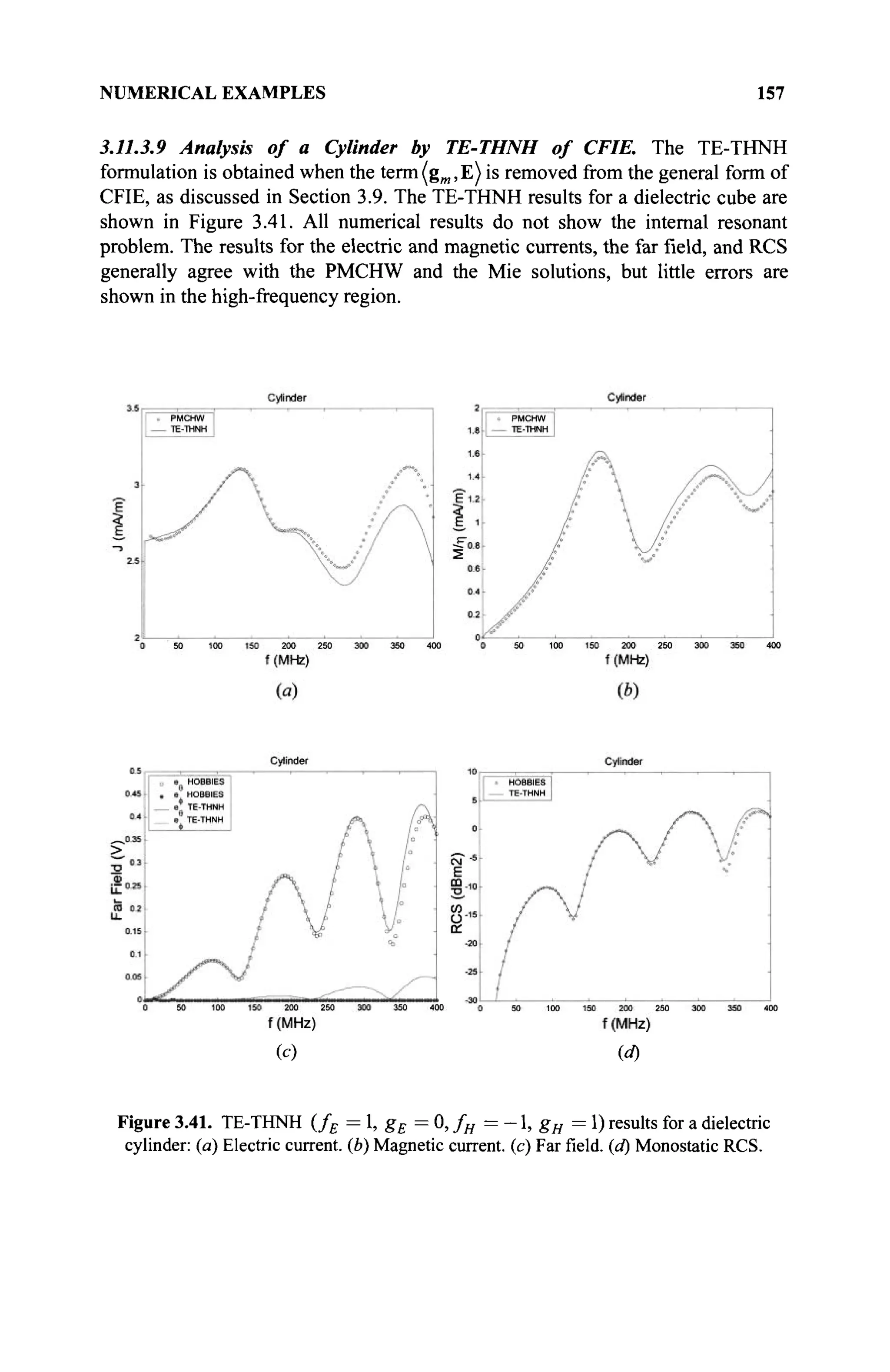
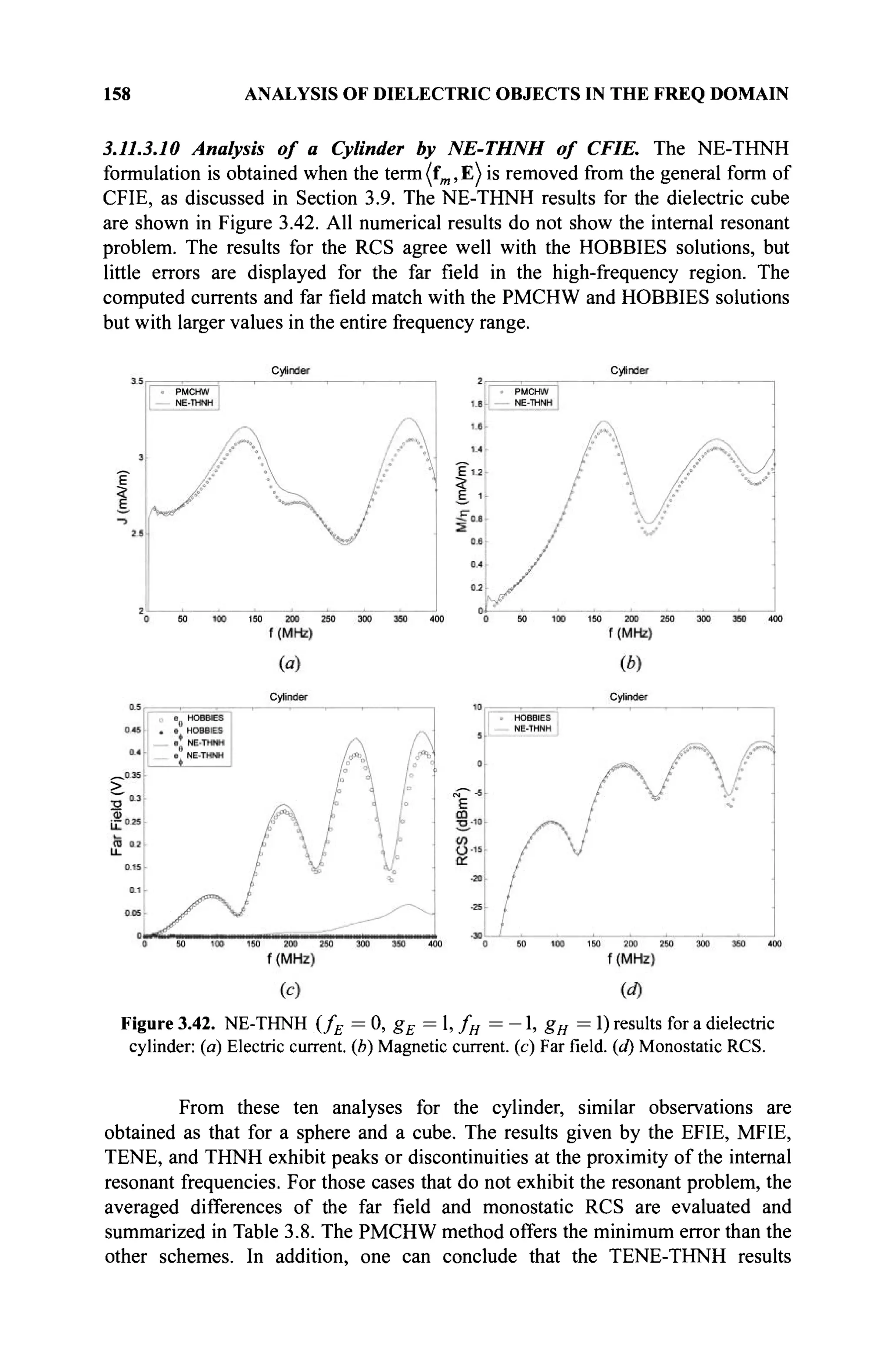
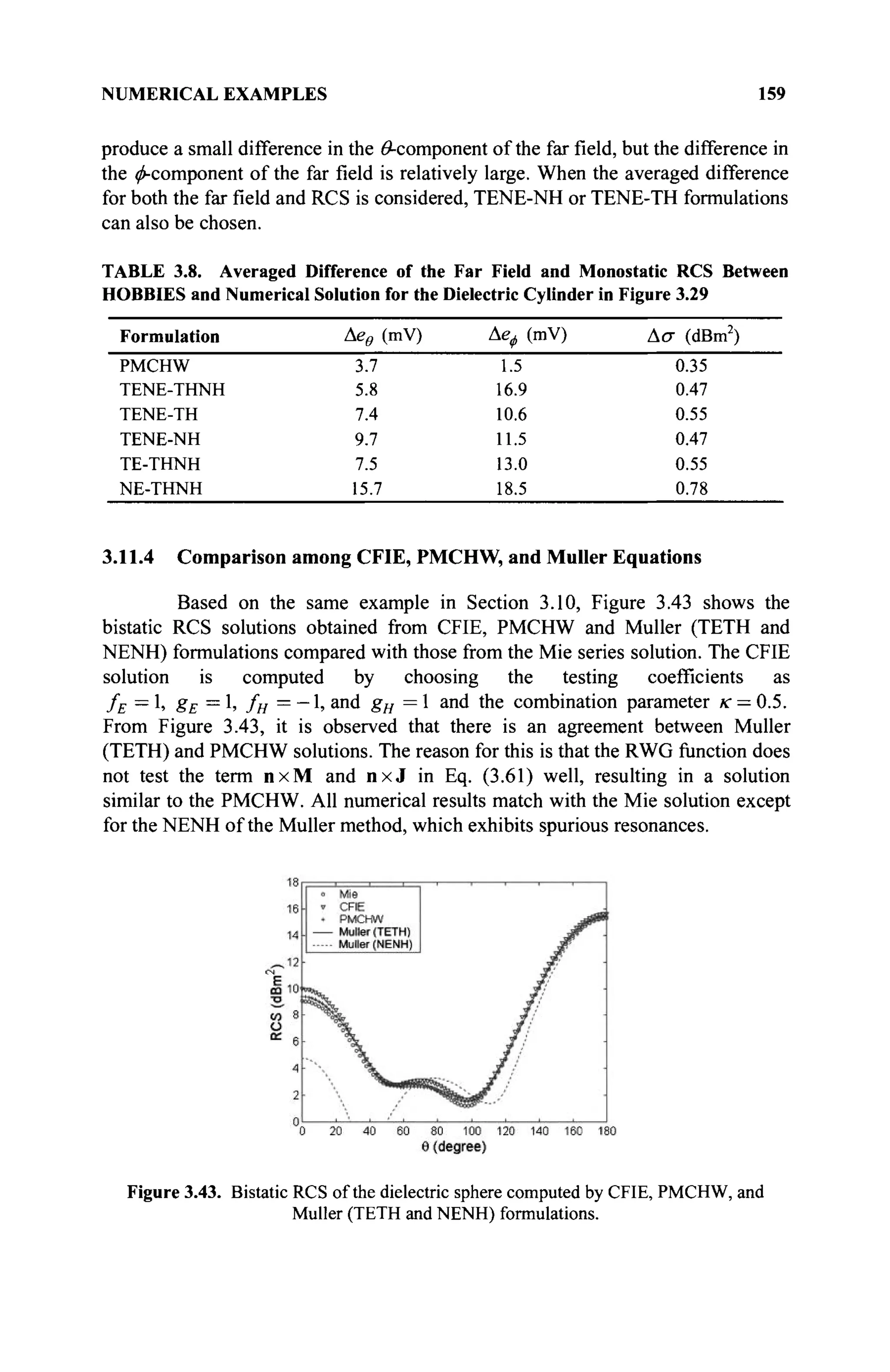
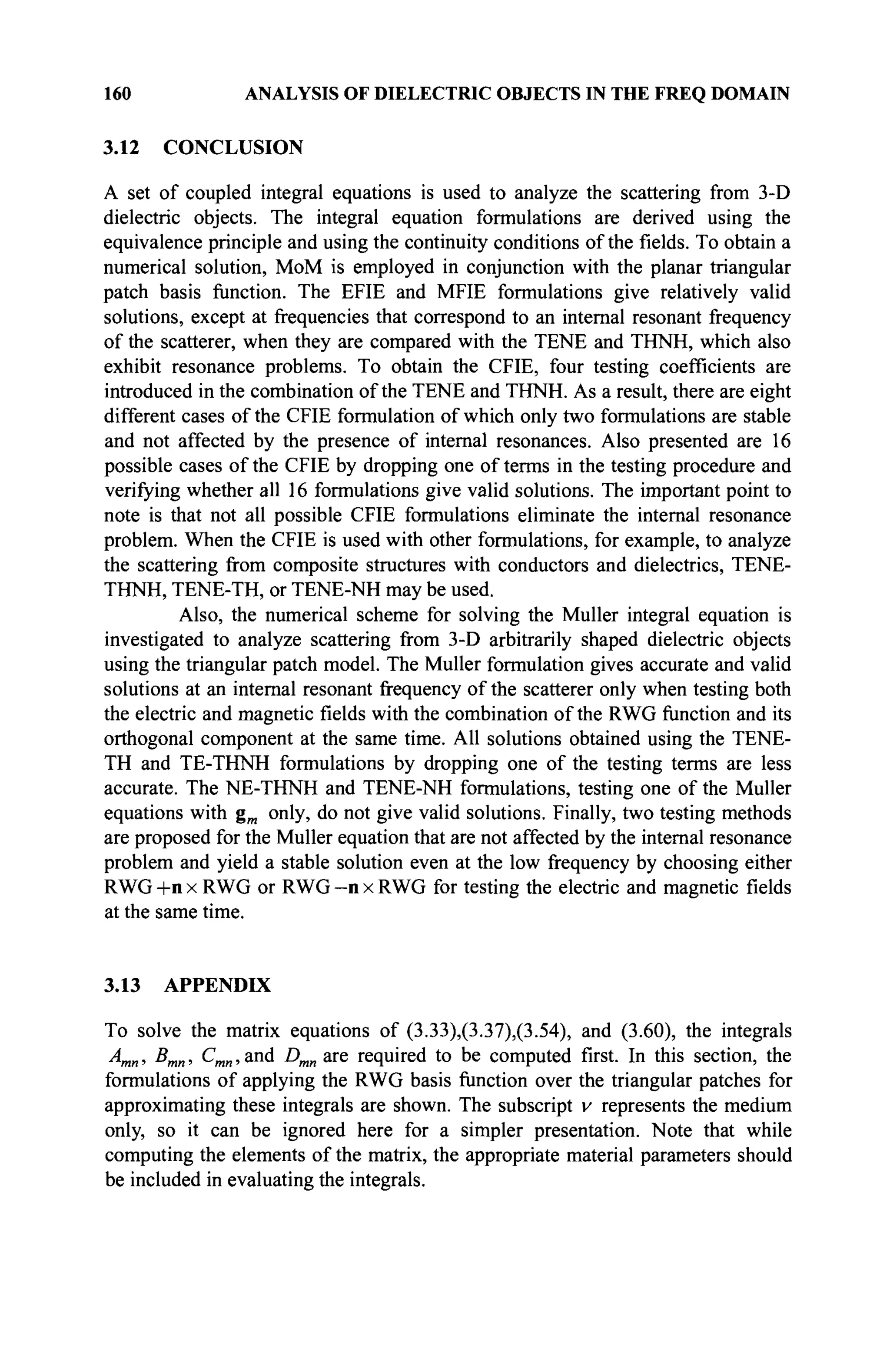
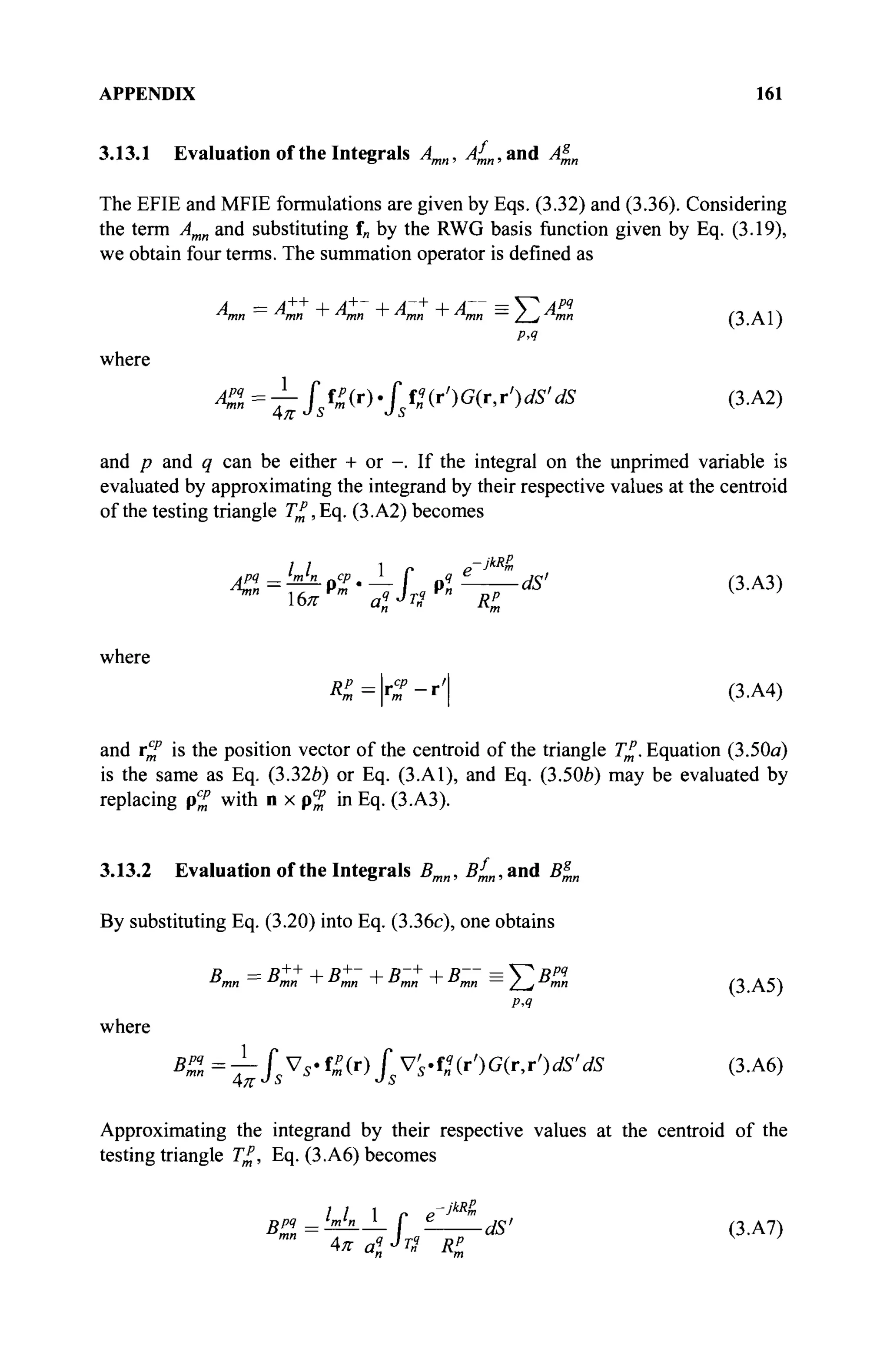
![162 ANALYSIS OF DIELECTRIC OBJECTS IN THE FREQ DOMAIN
where R% is given by Eq. (3.A4). Equation (3.50c) is the same as Eq. (3.36c) or
Eq. (3.A5). Equation (3.50d) is evaluated through
Rg
— V^ Rpq
-g
PA
where
BZ'g
~ Г nxf^(r) · fy's- Pn{r')VG{r,r')dS'dS (3.A9)
Approximating the integrand by the irrespective values at the centroid of the
testing triangle 7^,Eq. (3.A9) becomes
Bp4g =hnhLnxpp . J_ f y £ dS> (3.A10)
The evaluation of the potential integrals in Eqs. (3.A3), (3.A7), and (3.A10) may
be carried out by using the numerical methods specially developed for triangular
regions in [14-17].
3.13.3 Evaluation of the Integrals Cmn, c£,,and C^„
Using a vector identity [12], Eq. (332d) is given by
C m „ = ^ / / m ( r ) . n x ( n x f „ ( r ) ) ^ = - ^ i / 5 f ^ . f „ ^ 5 ( 3 .A 1 1 )
PA
The integral of Eq. (3.A11) can be computed analytically, and the result is given
by [18]
ifi-4*s
8a 4M +^иг
1Г+1г
2|2+
1г
зГ)~гС
'(г
'»+г
«)+г
'"'г
» (3.A12)
where r,, r2, and r3 are the position vectors for the three vertices of the triangle
T£ or T^, rc
is the centroid of the triangle T£ or Γ„?
, and A is the area of T£.
The vectors rm and r„ are the position vectors for the free vertex of the triangles
T£ and T%, respectively. Note that if the field point does not lie on the triangle
Γ„?
, (i.e. r ^ T4
), which results in C%j, =0. In Eq. (3.A12), the sign is positive
when p and q are same and negative otherwise.
Using the summation operator, Eq. (3.50e) is given by](https://image.slidesharecdn.com/timeandfrequencydomainsolutionsofemproblemsusingintegralequationsandahybridmethodologyb-250205130750-568a5ba2/75/Time-and-Frequency-Domain-Solutions-of-EM-Problems-Using-Integral-Equations-and-a-Hybrid-Methodology-B-H-Jung-pdf-184-2048.jpg)
![APPENDIX 163
Cl = 4 / / » ( г ) « nxf„(r)dS = ^ / s ^ · nxf„V5 ( з . А 1 3 )
By evaluating the element of Eq. (3.A13) analytically, the result is given by
i / s f £ .nxf„V5 = i ^ n . ( ( r m - r „ ) x r c
- ( r „ x r „ ) ) (3.A14)
By using a vector identity [18], Eq. (3.50/) may be written as
CL =ysnxfm(r).nxfn(r)dS = ^fsfZ(r).f!(r)dS ( 3 .A 1 5 )
Р.Ч
where the integral is same as in Eq. (3.A12).
Note that, if m and n does not belong to the same triangle, then Cm„ = 0.
And it is double of whatever expression one uses for it when m = n.
3.13.4 Evaluation of the Integrals Dmn, Df
mn, and D^n
By using the summation operator, the terms of Eq. (3.32e) are written as
D
"=T- f, f » * f,У x С ( г ) х У ' б ( г , г У 5 ' Л (З.А16)
where η' denotes the unit vector normal to the triangle T%. Thus, substituting Eq.
(3.19ft) into Eq. (3.A16), obtains
This integral may be computed using a Gaussian quadrature scheme over the
unprimed and primed coordinates numerically. Other integrals of Eqs. (3.50g),
(3.50/г), (3.58<Д and (b.59d) may be evaluated in a similar fashion.
3.13.5 Evaluation of the Integrals V^„, v£„, v£, V%, V^v, and V%v
Consider Eq. (3.32/) for v = 1 and apply a centroid testing, yielding
/5 fm (r).Ei
(r)^=J5 f+(r).Ei
(r)û ?S + J s f - ( r ) . E 1
( r ) ^](https://image.slidesharecdn.com/timeandfrequencydomainsolutionsofemproblemsusingintegralequationsandahybridmethodologyb-250205130750-568a5ba2/75/Time-and-Frequency-Domain-Solutions-of-EM-Problems-Using-Integral-Equations-and-a-Hybrid-Methodology-B-H-Jung-pdf-185-2048.jpg)
![164 ANALYSIS OF DIELECTRIC OBJECTS IN THE FREQ DOMAIN
= ^ ( ρ ^ . Ε 4 θ + ρΓ·Ε'(θ) (3.Α18)
Other integrals may be evaluated in a similar fashion.
REFERENCES
[I] R. F. Harrington, "Boundary integral formulations for homogeneous material
bodies," Jour. Electromagn. Waves Appl.,Vo. 3,pp. 1-15, 1989.
[2] K. Umashankar, A. Taflove, and S. M. Rao, "Electromagnetic scattering by
arbitrary shaped three-dimensional homogeneous lossy dielectric bodies," IEEE
Trans. Antennas Prop., Vol. 34, pp. 758-766, 1986.
[3] T. K. Sarkar, S. M. Rao, and A. R. Djordjevic, "Electromagnetic scattering and
radiation from finite microstrip structures," IEEE Trans. Microwave Theory Tech.,
Vol. 38, pp. 1568-1575, 1990.
[4] S. M. Rao and D. R. Wilton, "£-field, Я-field, and combined field solution for
arbitrarily shaped three-dimensional dielectric bodies," Electromagnetics, Vol. 10,
pp. 407-421, 1990.
[5] S. M. Rao, С. С. Cha, R. L. Cravey, and D. L. Wilkes, "Electromagnetic scattering
from arbitrary shaped conducting bodies coated with lossy materials of arbitrary
thickness," IEEE Trans. Antennas Prop., Vol. 39, pp. 627-631, 1991.
[6] X. Q. Sheng, J. M. Jin, J. M. Song, W. С Chew, and С. С. Lu, "Solution of
combined-field integral equation using multilevel fast multipole algorithm for
scattering by homogeneous bodies," IEEE Trans. Antennas Prop., Vol. 46, pp.
1718-1726, 1998.
[7] A. I. Mackenzie, S. M. Rao, and M. E. Baginski, "Electromagnetic scattering from
arbitrarily shaped dielectric bodies using paired pulse vector basis functions and
method of moments," IEEE Trans. Antennas Prop., Vol. 57, pp. 2076-2083, 1999.
[8] S. M. Rao, D. R. Wilton, and A. W. Glisson, "Electromagnetic scattering by
surfaces of arbitrary shape," IEEE Trans. Antennas Prop., Vol. 30, pp. 409^118,
1982.
[9] J. R. Mautz and R. F. Harrington, "Electromagnetic scattering from a homogeneous
material body of revolution," Arch. Elektron. Ubertragungstech., Vol. 33, pp. 71-
80, 1979.
[10] M. S. Yeung, "Single integral equation for electromagnetic scattering by three-
dimensional homogeneous dielectric objects," IEEE Trans. Antennas Prop., Vol.
47, pp. 1615-1622, 1999.
[II] Y. Zhang, and T. K. Sarkar, Parallel Solution of Integral Equation-based EM
Problems in the Frequency Domain, John Wiley & Sons, New York, 2009.
[12] R. F. Harrington, Time Harmonic Electromagnetics, McGraw-Hill, New York,
N.Y., 1961.
[13] B. H. Jung, T. K. Sarkar, and Y.-S. Chung, "A survey of various frequency domain
integral equations for the analysis of scattering from three-dimensional dielectric
objects,"/ Electromagn. Waves Appl, Vol. 16. pp. 1419-1421, 2002.
[14] D. R. Wilton, S. M. Rao, A. W. Glisson, D. H. Schaubert, О. M. Al-Bundak, and С.
M. Butler, "Potential integrals for uniform and linear source distributions on
polygonal and polyhedral domains," IEEE Trans. Antennas Prop., Vol. 32, pp.
276-281, 1984.](https://image.slidesharecdn.com/timeandfrequencydomainsolutionsofemproblemsusingintegralequationsandahybridmethodologyb-250205130750-568a5ba2/75/Time-and-Frequency-Domain-Solutions-of-EM-Problems-Using-Integral-Equations-and-a-Hybrid-Methodology-B-H-Jung-pdf-186-2048.jpg)
![REFERENCES 165
[15] S. Caorsi, D. Moreno, and F. Sidoti, "Theoretical and numerical treatment of
surface integrals involving the free-space green's function," IEEE Trans. Antennas
Prop., Vol. 41, pp. 1296-1301, 1993.
[16] R. D. Graglia, "On the numerical integration of the linear shape functions times the
3-D green's function or its gradient on a plane triangle," IEEE Trans. Antennas
Prop., Vol. 41, pp. 1448-1455, 1993.
[17] T. F. Eibert and V. Hansen, "On the calculation of potential integrals for linear
source distributions on triangular domains," IEEE Trans. Antennas Prop., Vol. 43,
pp. 1499-1502, 1995.
[18] S. M. Rao, Electromagnetic Scattering and Radiation of Arbitrarily-Shaped
Surfaces by Triangular Patch Modeling, PhD Dissertation, University Mississippi,
August, 1980.](https://image.slidesharecdn.com/timeandfrequencydomainsolutionsofemproblemsusingintegralequationsandahybridmethodologyb-250205130750-568a5ba2/75/Time-and-Frequency-Domain-Solutions-of-EM-Problems-Using-Integral-Equations-and-a-Hybrid-Methodology-B-H-Jung-pdf-187-2048.jpg)
![4
ANALYSIS OF COMPOSITE
STRUCTURES IN THE FREQUENCY
DOMAIN
4.0 SUMMARY
In this chapter, formulations are presented for the analysis of electromagnetic
scattering from an arbitrarily shaped three-dimensional (3-D) composite structure,
such as a perfectly conducting and piecewise homogeneous dielectric composite
body and the conducting object coated with dielectric material. The formulations
include the electric field integral equation (EFIE), the magnetic field integral
equation (MFIE), the combined field integral equation (CFIE), and the Poggio-
Miller-Chang- Harrington-Wu equation (PMCHW). To evaluate the efficacies of
different formulations, these integral equations are used to analyze four different
3-D composite scatterers, and their results are compared with each other as well as
a commercial software package, higher order basis function based integral
equations (HOBBIES). In the analysis, the equations are solved by using MoM
along with the triangular patch model and Rao-Wilton-Glisson (RWG) functions.
From the comparison, it is found that CFIE can approximate the HOBBIES
solution better than the EFIE and MFIE, particularly for preventing from spurious
solutions, which are found at the frequencies corresponding to internal resonances
of the structure.
4.1 INTRODUCTION
Many publications have reported the analysis of a composite structure that is a
combination of conducting and dielectric bodies. Some earlier techniques have
been used to solve two-dimensional problems and bodies of revolution [1-5]. In
addition, various methods using integral equations have been developed for 3-D
composite bodies [6-9]. There are four sets of coupled integral equations: the
EFIE, MFIE, CFIE, and the PMCHW equation. The EFIE, MFIE, and CFIE are
formed by considering only the electric fields, only the magnetic fields, or only the
electric and magnetic combined fields for the continuity conditions at both the
conducting and dielectric surface boundaries. In addition, different continuity
167
Time and Frequency Domain Solutions of EM Problems
Using Integral Equations and a Hybrid Methodology
by B. H. Jung, T. K. Sarkar, S. W. Ting, Y. Zhang, Z. Mei, Z. Ji,
M. Yuan, A. De, M. Salazar-Palma, and S. M. Rao
Copyright © 2010 John Wiley & Sons, Inc.](https://image.slidesharecdn.com/timeandfrequencydomainsolutionsofemproblemsusingintegralequationsandahybridmethodologyb-250205130750-568a5ba2/75/Time-and-Frequency-Domain-Solutions-of-EM-Problems-Using-Integral-Equations-and-a-Hybrid-Methodology-B-H-Jung-pdf-188-2048.jpg)
![168 ANALYSIS OF COMPOSITE STRUCTURES IN THE FREQ DOMAIN
conditions for the conducting and dielectric surfaces can be mixed to extend into
other forms of integral equations; for example, choosing the CFIE equation for the
conducting surface and the PMCHW equation for the dielectric surface, another
formulation is obtained and is called C-PMCHW. By changing the equations for
the conducting surface from CFIE to EFIE or to MFIE, new formulations called E-
PMCHW or H-PMCHW can be obtained.
Similar to the analysis of the 3-D conducting or dielectric objects using
the surface integral equations in Chapter 2 and 3, the integral equations can be
solved numerically by using method of moments (MoM) with the triangular patch
modeling and the RWG basis function [6]. Sarkar et al. proposed the EFIE for the
analysis of scattering by arbitrarily shaped 3-D complex bodies for the first time
[7]. In their work, the electric current is expanded using the RWG functions,
whereas the magnetic current is expanded using its point-wise spatially orthogonal
function, n x RWG Here n is the unit normal pointing outward from the surface.
In the testing procedure, the same RWG function is used.
In the analysis of conducting-dielectric composite bodies, spurious
solutions at the frequencies corresponding to an internal resonance of the structure
are found when only the EFIE or the MFIE is used. One possible remedy is to use
the combined field formulations. A CFIE formulation has been proposed by Sheng
et al. for a homogeneous dielectric problem [10]. In this work, the RWG functions
are used as basis functions to approximate both the electric and magnetic currents,
and RWG and n x RWG functions are used as testing functions. Based on Sheng's
work, Jung et al. presented a set of CFIE formulations by choosing a combination
of testing functions and dropping one of the testing terms in CFIE [11]. Using
these testing techniques, very good approximation to the exact solution has been
achieved without any internal resonant problems for the analysis of 3-D arbitrarily
shaped composite structures.
The problem of electromagnetic scattering from a coated structure that
consists of conducting objects enclosed by the dielectric material has been studied
extensively. Some techniques were proposed to solve two-dimensional and three-
dimensional structures [2,4,5,12]. The formulation EFIE-PMCHW [9,13], which is
the combination of EFIE for conducting boundaries and PMCHW formulation for
dielectric bodies, was proposed for the analysis of an arbitrarily shaped 3-D coated
structures. In the numerical solution procedures, the RWG function has been used
for both the basis and testing functions.
In this chapter, some particular choices of expansion and testing functions
for CFIE and PMCHW are introduced. Section 4.2 describes various integral
equations for analyzing composite structure and the suitable basis and testing
functions for them. Some numerical examples are given in section 4.3 for
composite structures to demonstrate the efficacies of the introduced formulations.
Sections 4.4 and 4.5 provide the equations and numerical examples for the
analysis of the scattering from coated structures. All examples here are compared
with the solutions from a commercial software package—HOBBIES [12]. Finally,
some conclusions are drawn in section 4.6.](https://image.slidesharecdn.com/timeandfrequencydomainsolutionsofemproblemsusingintegralequationsandahybridmethodologyb-250205130750-568a5ba2/75/Time-and-Frequency-Domain-Solutions-of-EM-Problems-Using-Integral-Equations-and-a-Hybrid-Methodology-B-H-Jung-pdf-189-2048.jpg)
![INTEGRAL EQUATION FOR COMPOSITE STRUCTURES 169
4.2 INTEGRAL EQUATIONS FOR COMPOSITE STRUCTURES
The integral equations for analyzing the composite structures are presented in this
section. The central idea of this analysis is to treat the composite object as many
individual conducting and dielectric bodies immersed in free space. To simplify
the presentation, it is assumed here that the composite structure consists of only
one conductor and one dielectric body, as shown in Fig. 4.1. The described
formulation for this case can be extended to apply for multiple complex structures.
Although the bodies shown in Figure 4.1 are separated, it generally is not
necessary to separate them. If the conducting and dielectric bodies are joined
together, then they are treated as two bodies with a zero-thickness layer of free
space separating them.
The composite structure in Figure 4.1 is illuminated by an incident plane
wave in which the electric and magnetic fields are denoted by E' and H'. The
incident field is defined as that would exist in space if the structure were not
present. The regions external and internal to the dielectric body are characterized
by the medium parameters (ε1,μι) and (^,/^λ respectively. The surfaces of the
conducting and dielectric scatterers are denoted by Sc and Sd. Furthermore, it is
assumed that the dielectric body is a closed body so that a unique outward normal
vector can be defined unambiguously.
Figure 4.1. A conducting-dielectric composite body illuminated by an electromagnetic
wave.
By using the equivalence principle [14], the conducting body is first
replaced by an equivalent surface current Jc radiating in the space (ελ,μχ). On
the conducting surface Sc, the total tangential electric field must approach zero.
The equivalent principle is employed next to split the original problem into two
parts, which are equivalent to the exterior and the interior region of the dielectric
body. In the equivalent problem for the exterior region, there is a restriction for the
fields external to the dielectric body that it should remain as the original, whereas
the fields inside the surface Sd can be chosen freely. For simplicity, the interior
fields are set to zero, and the entire interior region of the dielectric body is](https://image.slidesharecdn.com/timeandfrequencydomainsolutionsofemproblemsusingintegralequationsandahybridmethodologyb-250205130750-568a5ba2/75/Time-and-Frequency-Domain-Solutions-of-EM-Problems-Using-Integral-Equations-and-a-Hybrid-Methodology-B-H-Jung-pdf-190-2048.jpg)
![172 ANALYSIS OF COMPOSITE STRUCTURES IN THE FREQ DOMAIN
( l - a j ( - E U J c , J d , M ^ + a c 7 l ( j c - n x H ^ J c , J r f , M j )
= (l-ac)(E') +ae/71(nxH') forreS,
{l-ad)(-Es
]d(Jc,JdMd) + adVl(-Hs
ld(Jc,Jd,Mdj)
'tan V /tan
= (1-аДЕг
) +ad7h(H') forrGS,
V 'tan V 'tan
(1-^)(-Е^(Л^,М,)) i ^ i - H ^ i J r f . M , ) )
'tan V 'tan
= 0 for r 6 Sd
(4.5a)
(4.5b)
(4.5c)
where ηλ and /72 are the wave impedance of the exterior and interior region,
respectively. The parameters ac and ad are the usual combination parameters for
the boundary conditions enforced on the conducting and dielectric surfaces and
they can have any value between 0 and 1. When the conductor is open, the
parameter ac is set to zero and the formulation becomes EFIE.
An alternate formulation called C-PMCHW can be obtained by adding
Eq. (43b) to Eq. (4.3c) and Eq. (4.4b) to Eq. (4.4c), and using them in place of Eq.
(4.5Ä) and Eq. (4.5c), to yield
(4.6a)
(l-ac)(-KVc,*d,Md)^+acm(jc-nxnl(JcJd,Md))
= (1 - ac )(Ε' ) Ш + асщ (n x H' ) for r e Sc
(-Eirf(Jc.Jrf.M</)-E^(Ji,.Mrf))tBii=(E/
)taii f o r r e ^ (4.6Й)
(-Hfrf(Jc.J«/.Mrf)-Hi
M(Jrf,M(i))u|n=(H/
)tan f o r r e ^ (4.6c)
Note that Eq. (4.6a), which is obtained from the boundary condition on the
conducting surface Sc, is the same as Eq. (4.5a). Setting the combination
parameter ac in Eq. (4.6a) to extreme values leads to two special formulations
[5]:
• when ac = 0 , Eq. (4.6) is called E-PMCHW
• when ac=, Eq. (4.6) is calledH-PMCHW
To solve the described integral equations for composite objects, the
method of moment (MoM) along with a planar triangular patch model and RWG
functions are used, which have been applied for the pure conducting structure in
Chapter 2 and the pure dielectric structure in Chapter 3. To approximate the
electric or magnetic currents on the conducting and dielectric surfaces, the RWG
basis function f and its point-wise orthogonal vector basis function gn = n x fn](https://image.slidesharecdn.com/timeandfrequencydomainsolutionsofemproblemsusingintegralequationsandahybridmethodologyb-250205130750-568a5ba2/75/Time-and-Frequency-Domain-Solutions-of-EM-Problems-Using-Integral-Equations-and-a-Hybrid-Methodology-B-H-Jung-pdf-193-2048.jpg)
![INTEGRAL EQUATION FOR COMPOSITE STRUCTURES 173
can be used on each triangular patch, where n is the vector normal to the surface.
The electric currents Jc and Jd and the magnetic current Md on the scatterers
may be approximated in terms of these two basis functions as
Jc(r) = ^JC i „f„(r) (4.7a)
n=]
«d
Jd(r) = J2J
dJn+Nc(r) (4.7Ô)
я=1
Nd
Mrf(r) = £ M „ g n ( r ) (4.7c)
n=
where Nc and Nd are the numbers of common edges on the conducting and
dielectric surfaces in the triangular patch model, respectively. By choosing the
basis functions for the currents as Eq. (4.7) and the RWG function fm as the
testing function, the EFIE given by Eqs. (4.3) yields
(«m.-Efc ( J c ( U ^ ( U M ^ g , , ) ) ) = (fm,E'> (4-8fl)
(tm,-¥,'ld (jc(f„), Jd(fn)MAS„))) - (fm,E') (4Щ
( f ^ - E ^ G M U M ^ g j ) ) ^ (4.8c)
for m = 1,2, ..., Nc + Nd. For the MFIE formulation, the electric current Jc on the
conductor and the magnetic current M^ on the dielectric structure are expanded by
the function fw, whereas the electric current id is approximated by g„ as
Nc
Jc(r) = £XBf„(r) (4.9a)
*d
и=1
Nd
Md(r) = Y^M„fn+Nc(r) (4.9c)
»=1
The expansions of the currents on the dielectric surface in Eq. (4.9) are
dual to those in Eq. (4.7) for the EFIE formulation. The MFIE given by Eq. (4.4) is
expanded by using Eq. (4.9) and is tested with the RWG function fm, yielding
(fm,Jc(fJ-nxHîc(Jc(fI,),J<,(gI,),Mi/(fII))> = (f)„,nxH') ( 4 Л 0 а )](https://image.slidesharecdn.com/timeandfrequencydomainsolutionsofemproblemsusingintegralequationsandahybridmethodologyb-250205130750-568a5ba2/75/Time-and-Frequency-Domain-Solutions-of-EM-Problems-Using-Integral-Equations-and-a-Hybrid-Methodology-B-H-Jung-pdf-194-2048.jpg)
![174 ANALYSIS OF COMPOSITE STRUCTURES IN THE FREQ DOMAIN
(fm,-HL(Jc(fnX^(g«XMrf(f„))) = (fm,H'') (4Лое)
fc.-H^ (Jrf(8B),Mrf(f„))) = 0 (4.10c)
Now consider the CFIE formulation. All the currents Je , Jd, and M^ are
expanded by the RWG basis function f„ as
Nc
Jc(r) = £ X „ f „ ( r ) (4.11«)
n=
Nd
Jd(r) = 2ÏJdJn+Ne(r) (4Mb)
Nd
М,(г) = £ м Л ( г ) (4.11с)
«=i
In the CFIE formulation, Eq. (4.5a) is tested with fm, and a combination of fm and
gm are used as the testing functions for Eqs. (4.5Й) and (4.5c). By choosing the
testing functions for the electric field part as fm + gm and for the magnetic field part
as -fm + gm [11], we obtain
( l - « c ) ( f m , - E ^ J c ( f „ ) , J ^ U M ^ ( f „ ) )
+асП] (fm, Jc (f„ ) - n x Щс (je (f„ ), Jd (f„ ), Md (f„ )))
= «c?
7i(f
m>n
xH
'') + (1
-«c)(f
™,E'') (4.i2a)
(!-««/)('»+g,».-EÎ<i(Jc(f»).Jrf(f»).Mi/(f„)))
+««/7. ("f
m + gm> -Ηί Л Jc & ), J Л*„ ), Md (f„ )))
= «I /'7i(-fm +gm ,H/
) + (l-ad )(fm +gm ,E/
) ( 4 J 2 è )
(l-ar f )(fm +gB ,-E'M (Jr f (UMr f (i»))
+ а д 2 (-fm +gB,,-H,
2(/ (Jd(f„),Mrf(f„)))
= 0 (4.12c)
Note that it is also possible to choose the testing functions as fm — gm for the
electric field part and fm +gm for the magnetic field part [11]. Setting the
combination parameters ac and ad in Eq. (4.12) to extreme values leads to the
following special formulations [10,11]:](https://image.slidesharecdn.com/timeandfrequencydomainsolutionsofemproblemsusingintegralequationsandahybridmethodologyb-250205130750-568a5ba2/75/Time-and-Frequency-Domain-Solutions-of-EM-Problems-Using-Integral-Equations-and-a-Hybrid-Methodology-B-H-Jung-pdf-195-2048.jpg)
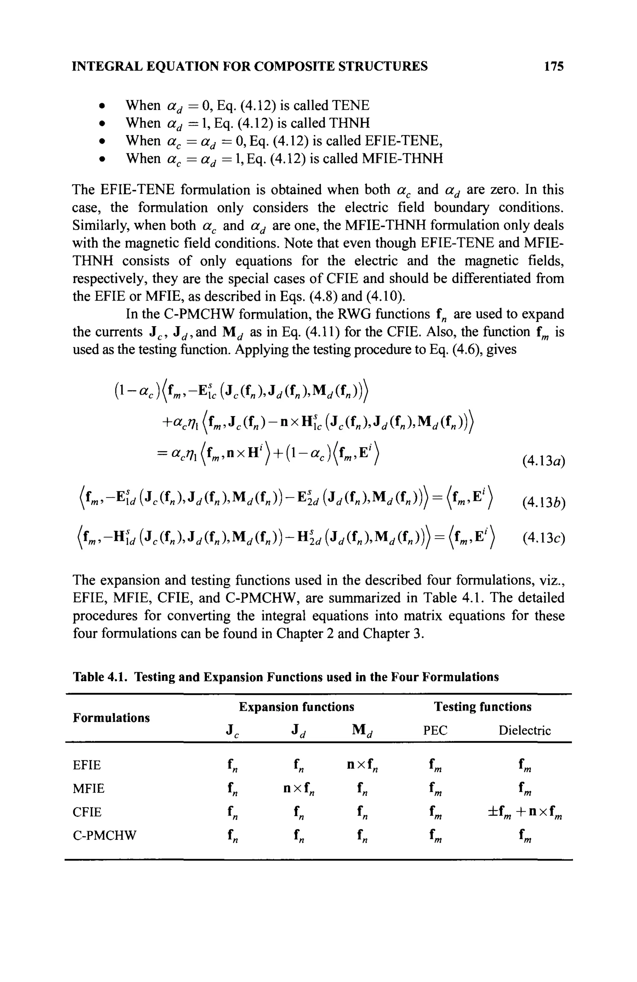
![176 ANALYSIS OF COMPOSITE STRUCTURES IN THE FREQ DOMAIN
To summarize this section, the EFIE, MFIE, CFIE, and C-PMCHW
(including E-PMCHW and H-PMCHW) formulations are given by Eqs. (4.3),
(4.4), (4.5), and (4.6), Using the testing functions as listed in Table 4.1, the testing
of these integral equations for these four cases result in Eqs. (4.8), (4.10), (4.12),
and (4.13), respectively.
4.3 NUMERICAL EXAMPLES FOR COMPOSITE OBJECTS
In this section, the numerical results obtained from the integral equations for
composite objects described in the previous section are presented and compared.
In the numerical computations, the scatterers are illuminated from the top (—z
direction) by an incident x-polarized plane wave. The frequency range, over which
the results are calculated, is between 0 MHz to 500 MHz at an interval of 4 MHz.
All computed results are compared with the solution obtained from a commercial
software package, HOBBIES [12], at the same interval of 4 MHz.
The first example is a composite sphere structure as shown in Figure 4.2,
which consists of a perfectly-electric-conducting (PEC) sphere and a dielectric
sphere. The conducting sphere has a diameter of 1 m and is centered at the origin
of the coordinates. The dielectric has a diameter of 0.8 m and a relative
permittivity of er =2. The separation between their centers is 1 m. The surface of
each sphere is modeled by 528 triangular patches, which results in 792 edges. The
total number of unknowns for the whole structure is N = Nc +2Nd = 2376. In
HOBBIES, a similarly number of unknowns, 2304, is used for computation.
Figure 4.2. A composite sphere structure consisting of a PEC sphere with a diameter of 1
m and a dielectric sphere with a diameter of 0.8 m and er=2.
Figure 4.3 shows the comparison of the radar cross-section (RCS)
solution obtained from the EFIE and MFIE, with the solution from HOBBIES.
The figure shows that there are several discontinuities in both the EFIE and MFIE](https://image.slidesharecdn.com/timeandfrequencydomainsolutionsofemproblemsusingintegralequationsandahybridmethodologyb-250205130750-568a5ba2/75/Time-and-Frequency-Domain-Solutions-of-EM-Problems-Using-Integral-Equations-and-a-Hybrid-Methodology-B-H-Jung-pdf-197-2048.jpg)
![NUMERICAL EXAMPLES FOR COMPOSITE STRUCTURES 177
results, which exhibit at the internal resonant frequencies of the two spheres.
Besides these discontinuities, both the EFIE and MFIE agree with the HOBBIES
solution.
Figure 4.3. Comparison of monostatic RCS for the composite sphere structure computed
by the EFIE and MFIE formulations along with the HOBBIES solution.
Figure 4.4 compares the results from HOBBIES solution with the special
cases of the CFIE that relates only to either the electric or the magnetic field (i.e.,
EFIE-TENE [when ac = ad = 0] and MFIE-THNH [when ac = ad = 1]), in
comparison to the. For the latter formulations, discontinuities are still observed at
the internal resonant frequencies. At other frequencies, the results from EFIE-
TENE and MFIE-THNH are in good agreement with the HOBBIES solution.
Figure 4.4. Comparison of monostatic RCS for the composite sphere structure computed
by EFIE-TENE (CFIE with ac = ad = 0 ) and MFIE-THNH (CFIE with ac = ad = 1 )
formulations along with the HOBBIES solution.](https://image.slidesharecdn.com/timeandfrequencydomainsolutionsofemproblemsusingintegralequationsandahybridmethodologyb-250205130750-568a5ba2/75/Time-and-Frequency-Domain-Solutions-of-EM-Problems-Using-Integral-Equations-and-a-Hybrid-Methodology-B-H-Jung-pdf-198-2048.jpg)
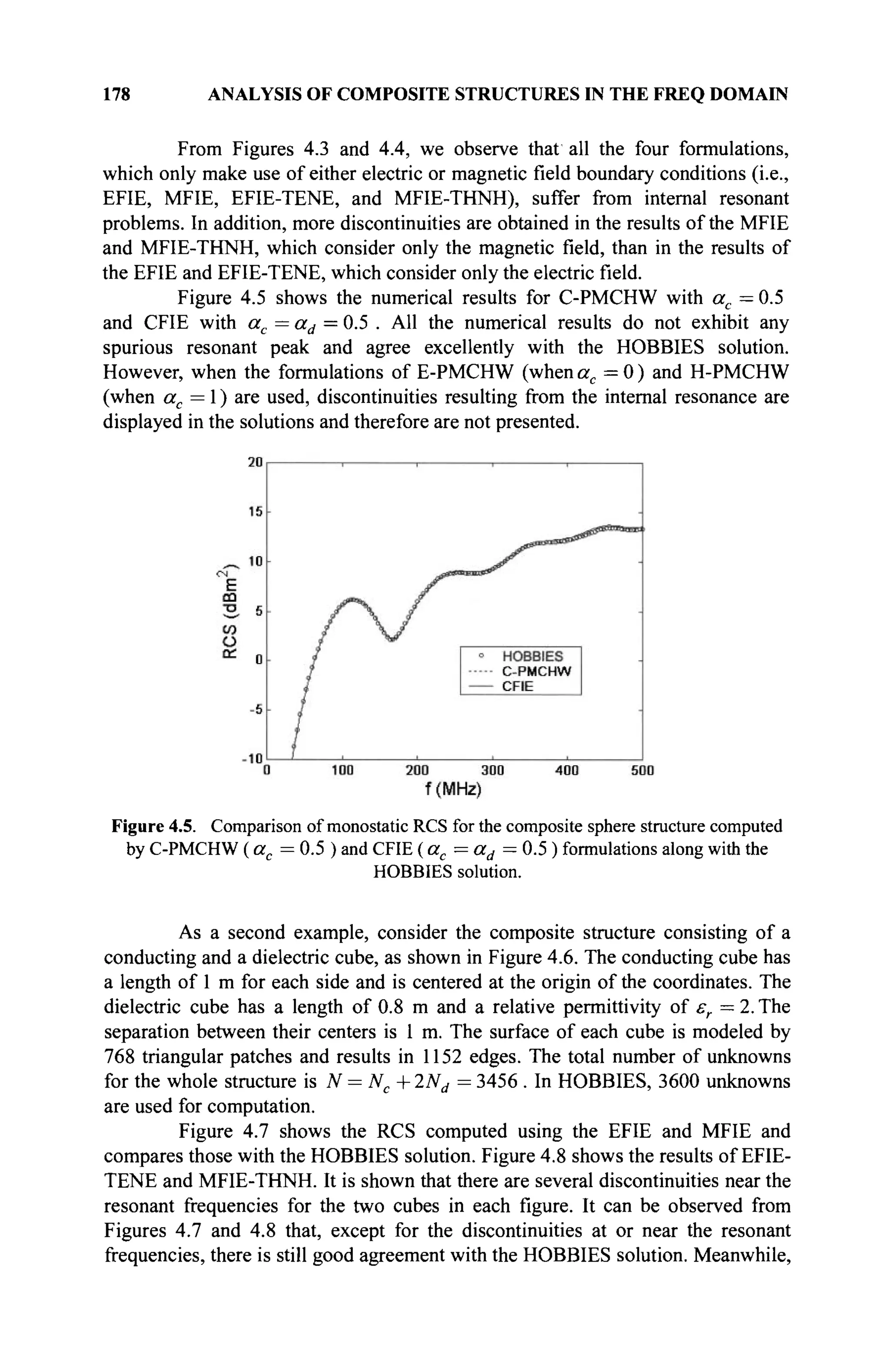
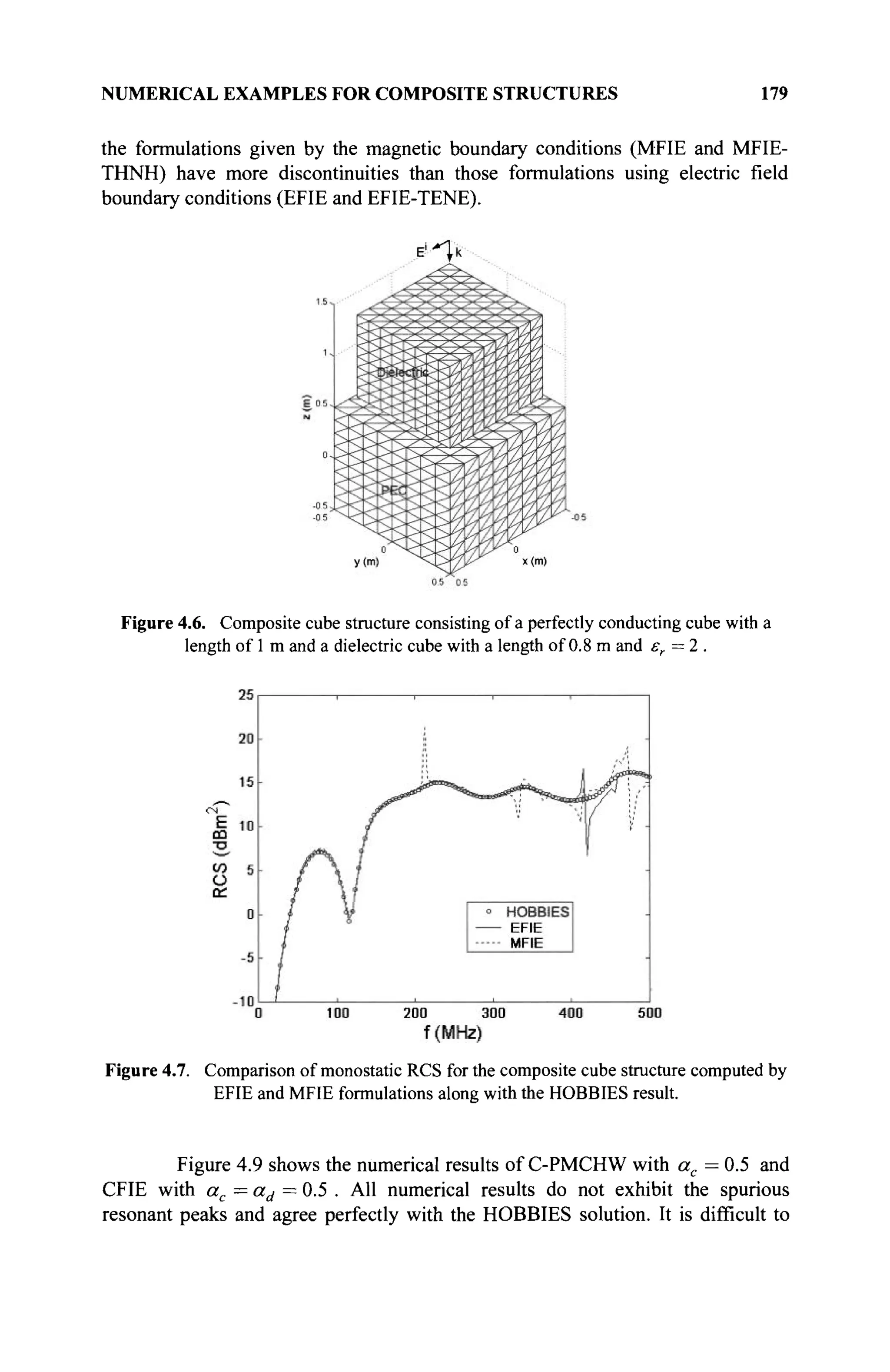
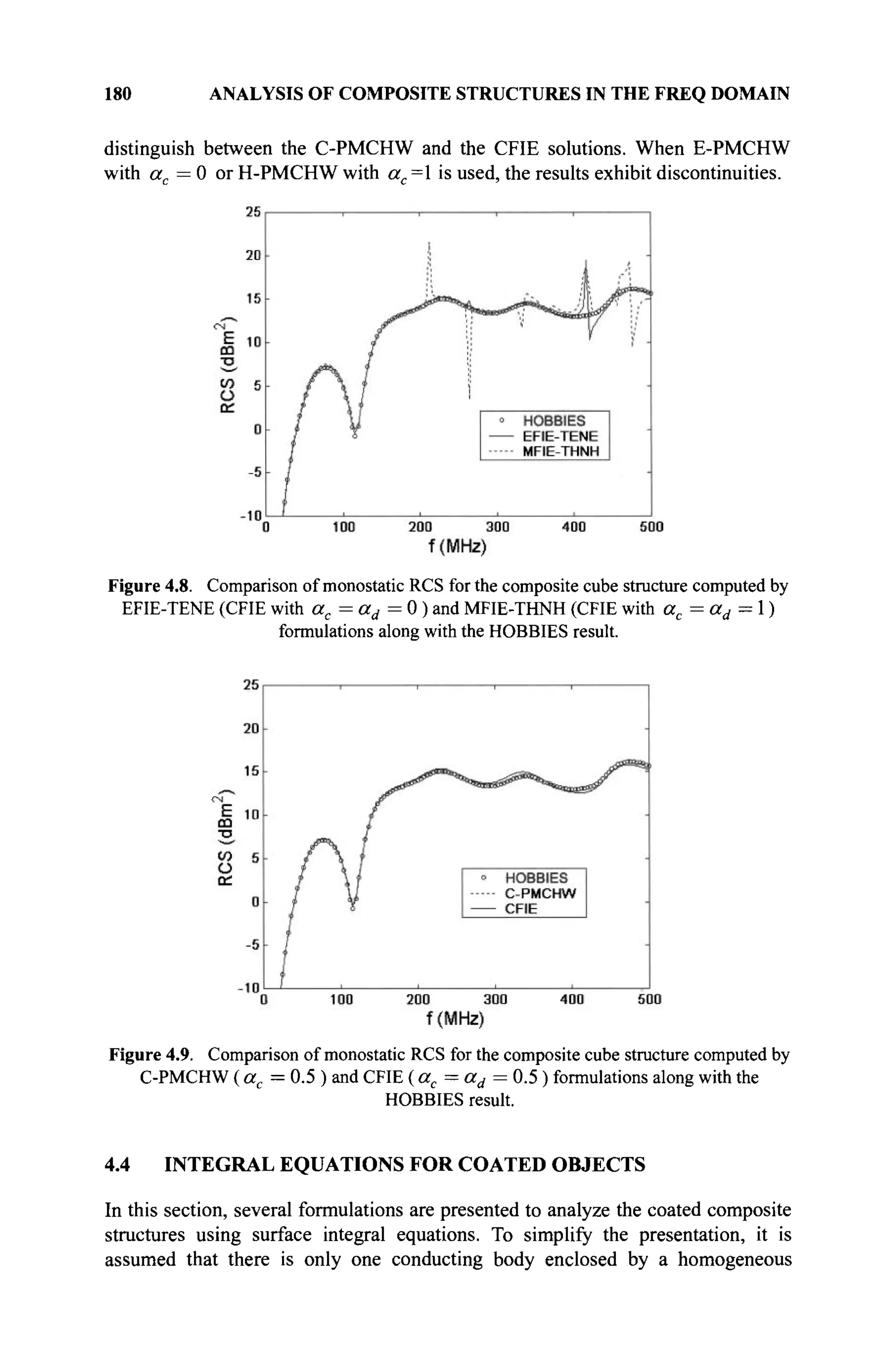
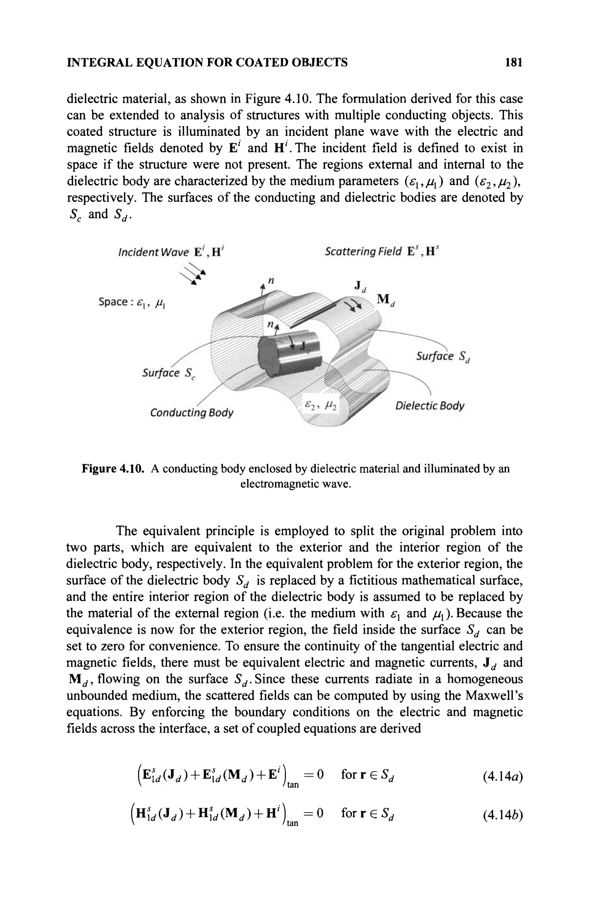
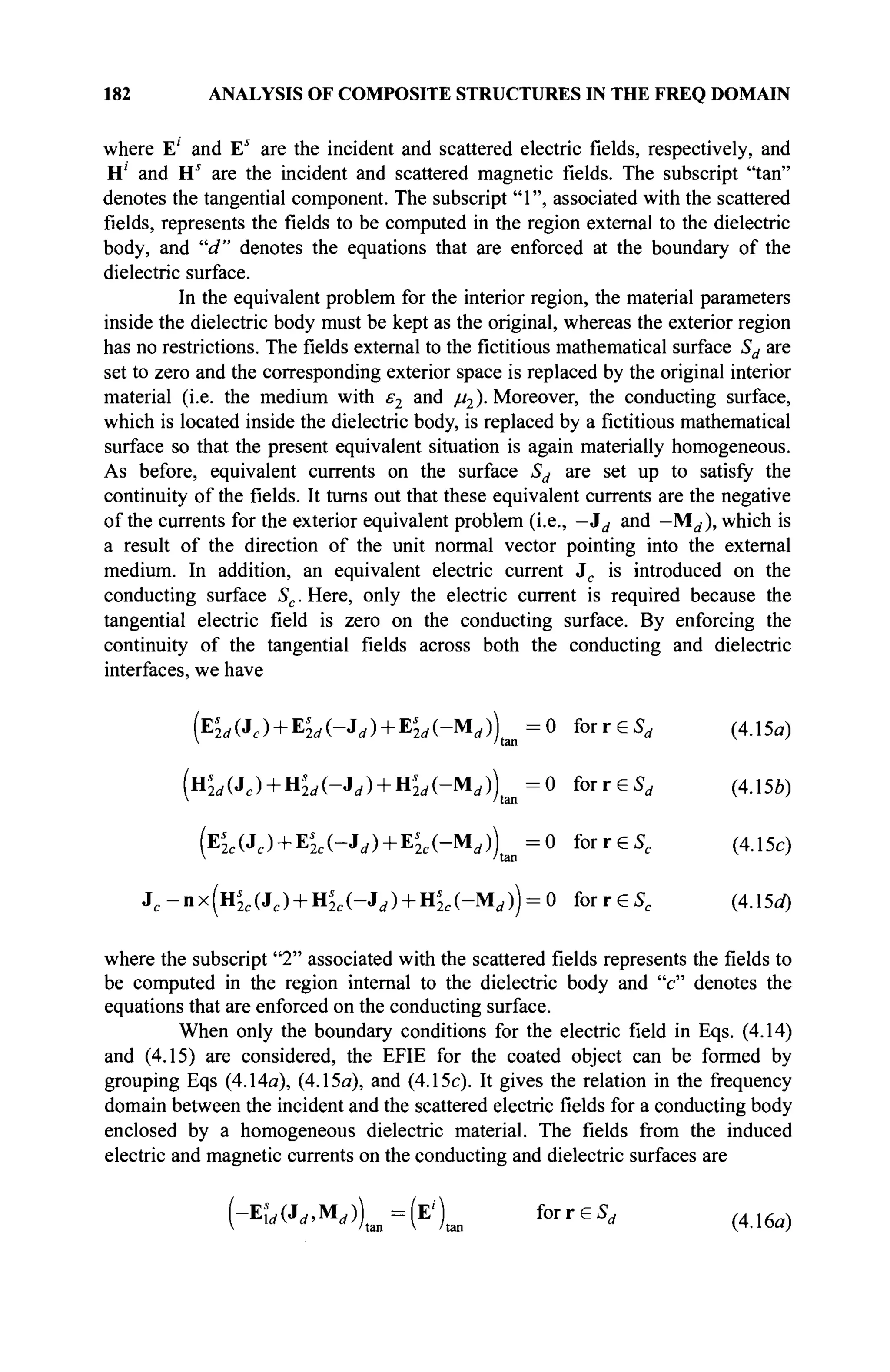
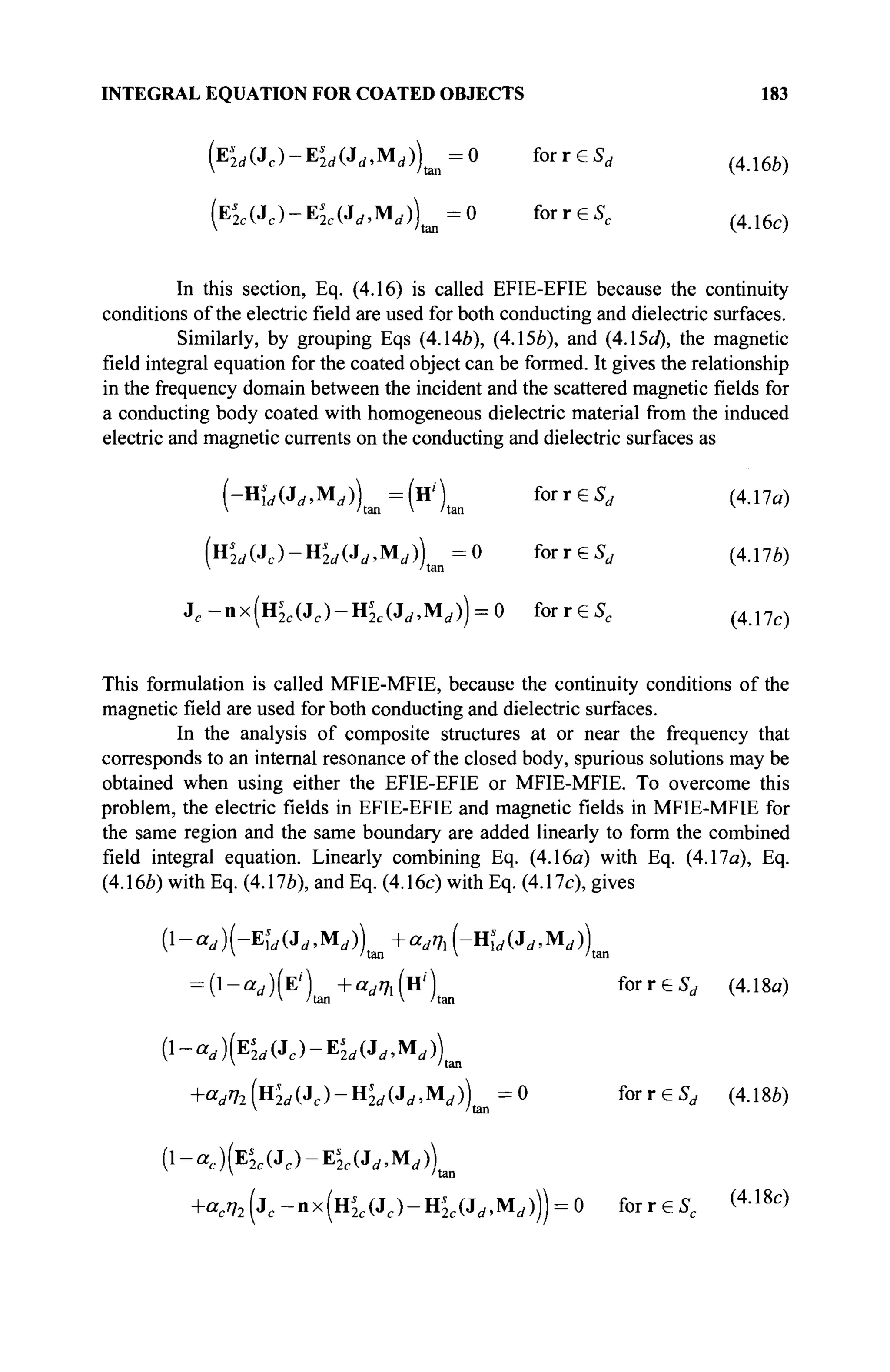
![184 ANALYSIS OF COMPOSITE STRUCTURES IN THE FREQ DOMAIN
where 77, and η2 are the wave impedance of the exterior and interior regions. The
parameter ac and ad are the usual combination parameters that can be assigned
to any value between 0 and 1. This formulation is called CFIE-CFIE because the
continuity conditions of the combined electric and magnetic fields are used for
both the conducting and dielectric surfaces. For the open conducting structure, ac
needs to be set to zero and this results in EFIE-CFIE formulation.
An alternative way to combine the electric and magnetic field
formulations, the electric fields in EFIE-EFIE evaluated at the boundary of the
dielectric surface Sd are added linearly. Similar summation is also performed for
the magnetic fields in MFIE-MFIE. By linearly adding Eq. (4.16a) to Eq. (4.16Й)
and Eq. (4.17a) to Eq. (4.17*), the CFIE-PMCHW formulation is obtained
(-Ei,(J.,Mi / )-Ei
2 t / (Jt / ,M( i ) + Ei
2rf(Jc))tan=(E')tan for г e $ , (4.19α)
(-Uld(Jd,Md)-Hs
2d(Jd,Md) + ns
2d^c)m=(^Xn for r e S , (4.196)
{-ac)(E2c(Jc)-Es
2c(Jd,MA
/tan
+«e % (jc -nx(H2 c (Jc )-H2 e (Ji / ,M( / ))) = 0 forreSc (4 Л 9 с
)
Note that Eq. (4.19c), which is derived at the boundary of the conducting surface
Sc, is kept the same as Eq. (4.18c). The formulation given by Eq. (4.19) is called
E-PMCHW when the parameter ac in Eq. (4.19c) is zero, or it is called H-
PMCHW when ac is equal to one [5].
To solve the resulting equations obtained for coated objects, the method
of moment along with the triangular surface patch model and the RWG basis
functions are used. The expansion and testing functions for these formulations are
chosen the same as those for the composite objects, and one can refer to Table 5.1
for more information.
Similar to the EFIE formulation for the composite objects, the electric
current Jc and Jd and the magnetic current M^ in EFIE-EFIE formulation given
by Eq. (4.16) are approximated by Eq. (4.7) and tested with fm and yield
(fm,"Ew (MUMrfte,))) = (fm,E'") (4.20a)
{L^IJ (Jc(fJ)-EL (-UUMd(g„))) = 0 (4.20b)
(f„,E*2c (Jc(fB))-E£c (.Μυ,Μ,(8„))) = 0 (4.20c)
For the MFIE-MFIE formulation given by Eq. (4.17), the equivalent electric
current Jc on the conductor, the electric current Jd, and the magnetic current M^
may be expanded by Eq. (4.9) and tested with fm, yielding](https://image.slidesharecdn.com/timeandfrequencydomainsolutionsofemproblemsusingintegralequationsandahybridmethodologyb-250205130750-568a5ba2/75/Time-and-Frequency-Domain-Solutions-of-EM-Problems-Using-Integral-Equations-and-a-Hybrid-Methodology-B-H-Jung-pdf-205-2048.jpg)
![INTEGRAL EQUATION FOR COATED OBJECTS 185
( Ъ . - Η ί , (Jrf(8„).Mrf(f„))) = (fm,H') (4.21a)
(f».H^(Jc (f
»))-H
M(^(g»).M< / (fl ,))) = 0 (4.21b)
( ^ . J ^ f J - n x f H ^ ^ i f j J - H ^ ^ i g J . M ^ f j J ^ O (4.21c)
Consider the CFIE-CFIE formulation now. The equivalent currents Jc ,
Jd,and M^ are all approximated by the RWG basis function f„ as given by Eq.
(4.11 ). Two vector basis functions are used in the testing for the fields at the dielectric
surface. By choosing the testing functions for electric field part as fm + gm and for
the magnetic field part as —
f
m +gm [11], the CFIE-CFIE formulation given by Eq.
(4.18) results in
^-ccd){fm+gm,-Es
ld(Jd(t„)MAfJ))
+ W - f
» + 8 » > - H w ( J
r f ( U M < i ( f B ) ) )
' (4.22a)
= (l-arf)(fm+gm»E,
') + ar f 7,(-fm +gm ,Hi
)
(l-«</)(fB,+gm.Ej</(Jc(fn))-E,
2i,(Jrf(f»).Mrf(f„)))
+<V72(-fm +g„.HL(Jc(f»))-H^(Jrf(f»).Mrf(f„))) = 0 (4.22U)
(1 - ac )(fm,Es
2c (Jc (f„ )) - EL (j„ (f„ ),M„ (f„ )))
+acV2 (fm, Jc (f„)-nx(H2 c (Jc (f„))-Hk (Jrf(f„).Mrf(f„)))) = 0 (4
-22c
)
Note that Eq. (4.22c) is tested with only RWG function for the conducting surface.
In the CFIE-PMCHW formulation, the procedure is the same as CFIE-
CFIE; the RWG functions f„ are used to expand all the equivalent currents Jc
id, and Μ^, and fm is used as the testing function. Applying the testing procedure
to Eq. (4.19), we obtain
- E L {Jd(OMAO) + Kd (Jc(f„))) = (ί,,Ε') (4.23α)
(fm,-Hs
ld(jd(fn),MAO)
-ns
2d (J,(f„),M,(f„)) + HL (Je(f„))) = (fm,H<) (4.23Й)](https://image.slidesharecdn.com/timeandfrequencydomainsolutionsofemproblemsusingintegralequationsandahybridmethodologyb-250205130750-568a5ba2/75/Time-and-Frequency-Domain-Solutions-of-EM-Problems-Using-Integral-Equations-and-a-Hybrid-Methodology-B-H-Jung-pdf-206-2048.jpg)
![186 ANALYSIS OF COMPOSITE STRUCTURES IN THE FREQ DOMAIN
(l-oc)(fw>EI
2c(Jc(fB))-EI
2c(ji/(fB),M(/(fII))> + aci72<f».Jc(f»)
-nx(Hs
2c {Jc(t„))-^'2c (Jd(f„XM,(f„)))) = 0 (4.23c)
Note that Eq. (4.23) can be converted into a matrix equation for the CFIE-
PMCHW formulation. A detail procedure to convert the integral equations into a
matrix equation can be found in [11]. In this section, the formulation for analyzing
the scattering of a coated structure was presented. The EFIE, MFIE, CFIE, and C-
PMCHW formulation are given by Eqs. (4.16), (4.17), (4.18), and (4.19),
respectively. Using the expansion and testing functions listed in Table 5.1, the
testing of the integral equations for these four cases result in Eqs. (4.20), (4.21),
(4.22), and (4.23), respectively.
4.5 NUMERICAL EXAMPLES FOR COATED OBJECTS
In this section, the numerical results obtained from the formulations for coated
objects described in the previous section are presented and compared. In the
numerical computations, the scatterers are illuminated from the top ( —z direction)
by an incident x -polarized plane wave. The frequency range, over which the RCS
is calculated, is between 0 MHz to 500 MHz at an interval of 4 MHz. All
computed results are compared with the solution obtained from a commercial
software package, HOBBIES [12], at the same interval of 4 MHz.
The first example is a conducting disk enclosed by a dielectric cylinder,
as shown in Figure 4.11. The conducting disk has a radius of 0.4 m and is centered
at the origin of the coordinates. The dielectric cylinder has a radius of 0.5 m and a
height of 0.5 m. The relative permittivity is er =2 . The surface of the conducting
disk is modeled with 160 triangular patches, which results in a total of 240
common edges. The outer surface of the dielectric cylinder is modeled with 528
triangular patches and has a total of 792 edges. The total number of unknowns for
the whole structure is N = Nc +2Nd =1824. The number of unknowns is 2134
in the computation using HOBBIES.
Figure 4.11. A conducting disk with a radius of 0.4 m enclosed by a dielectric cylinder
( er = 2 ) with a radius of 0.5 m and a height of 0.5 m.](https://image.slidesharecdn.com/timeandfrequencydomainsolutionsofemproblemsusingintegralequationsandahybridmethodologyb-250205130750-568a5ba2/75/Time-and-Frequency-Domain-Solutions-of-EM-Problems-Using-Integral-Equations-and-a-Hybrid-Methodology-B-H-Jung-pdf-207-2048.jpg)
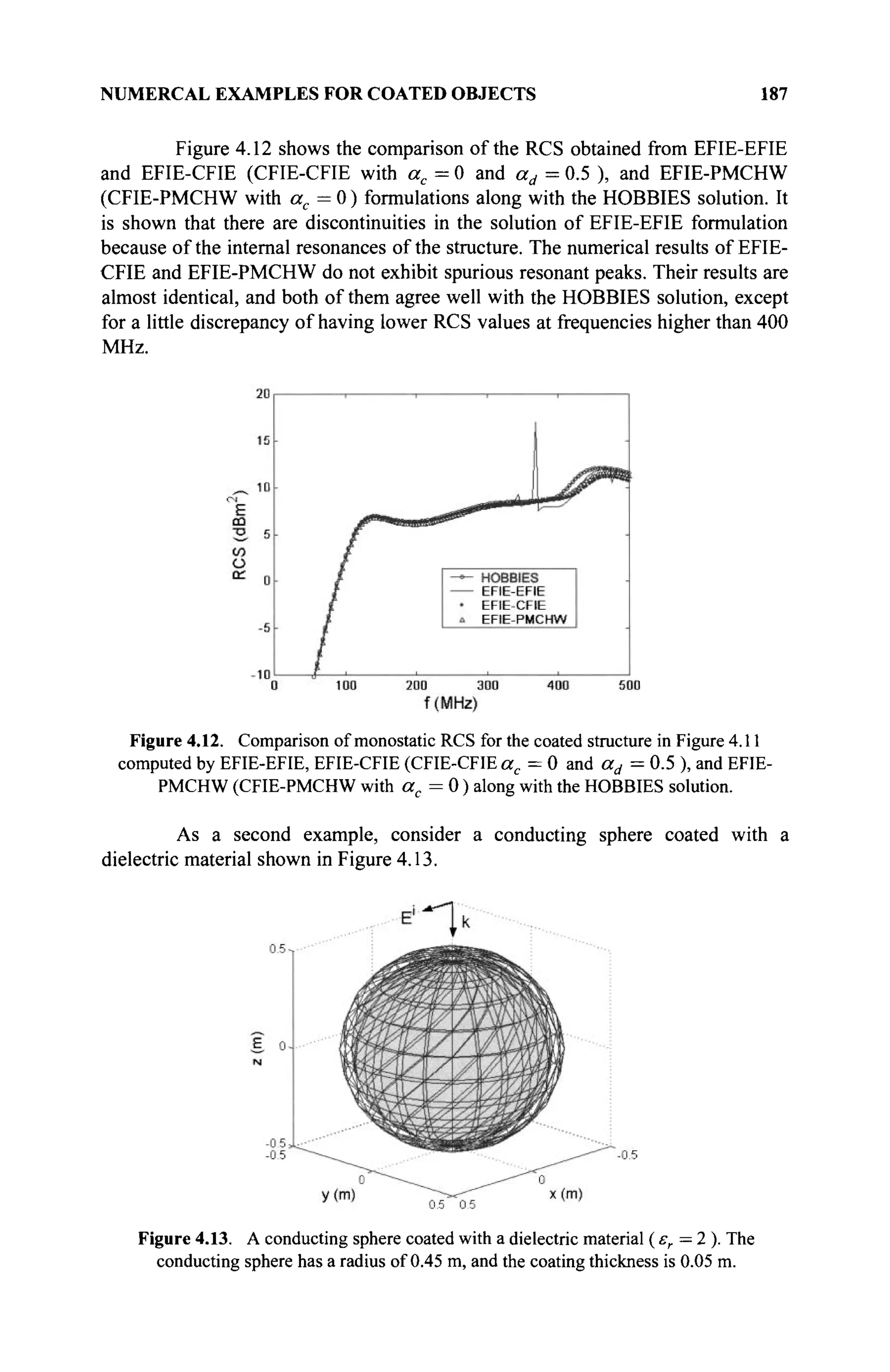
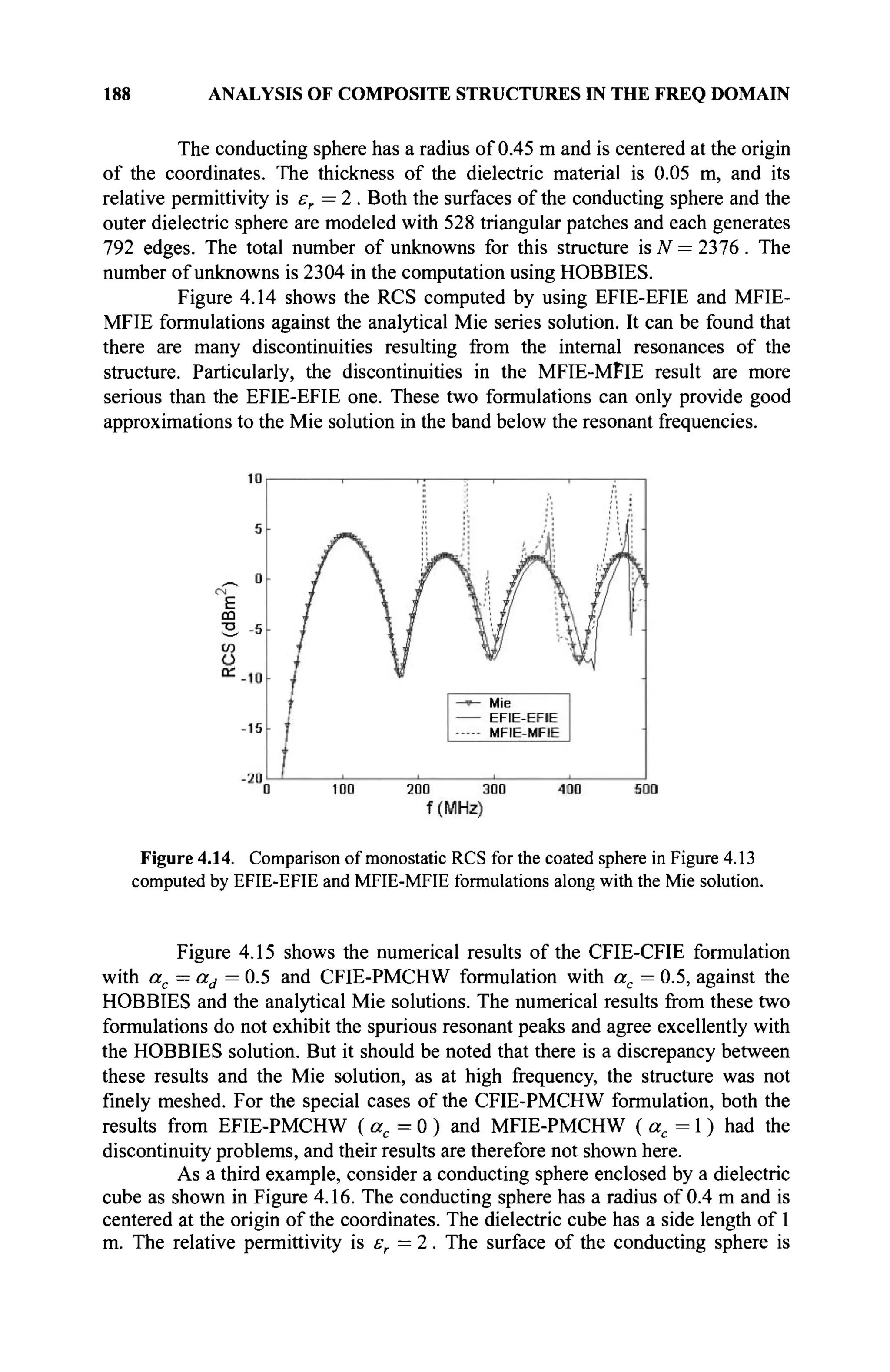
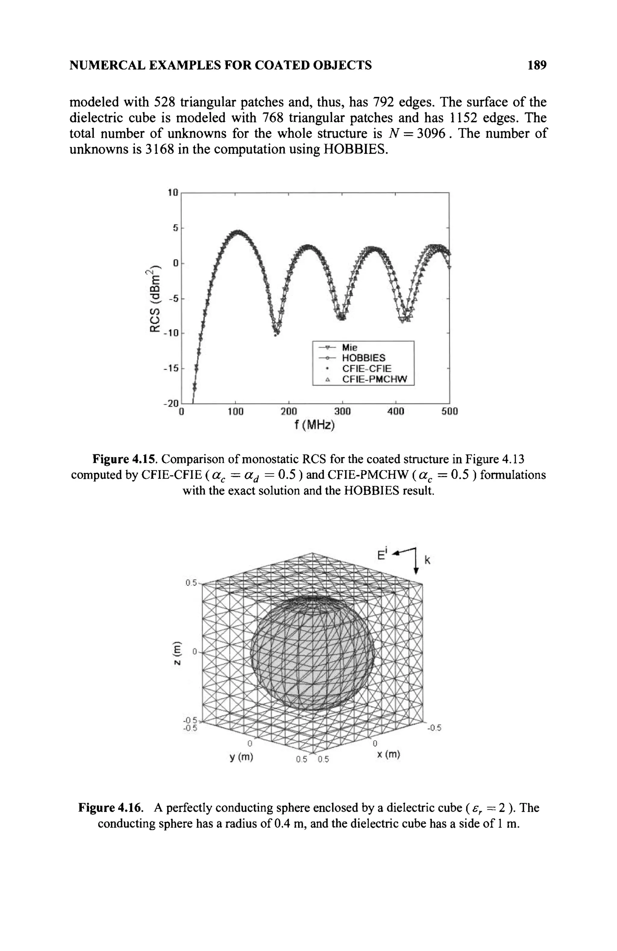
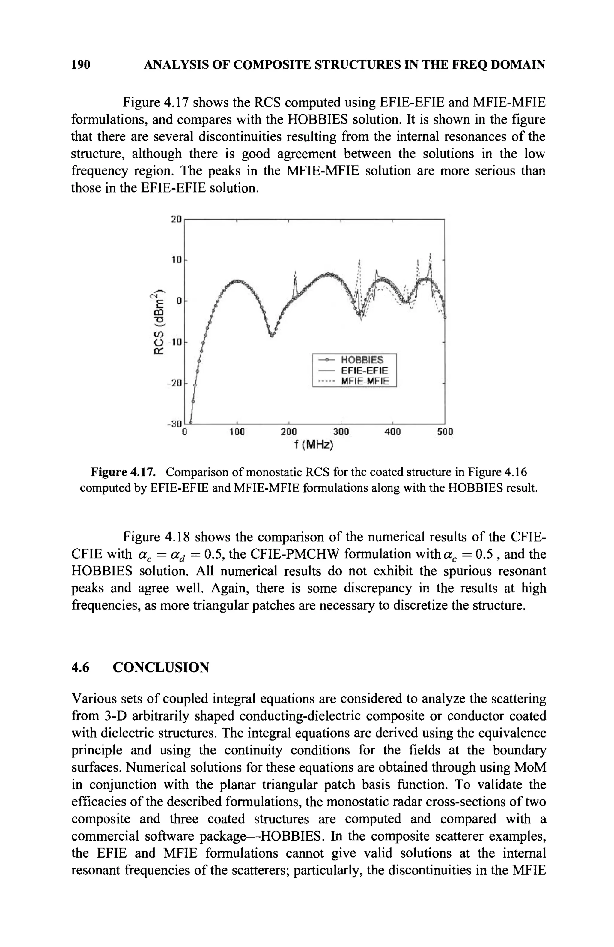
![REFERENCES 191
results are relatively larger. Although stable solutions can be obtained by using the
CFIE and C-PMCHW formulations and they have excellent agreements with the
HOBBIES solutions. From the three examples of the coated structure, it is found
that EFIE-EFIE and MFIE-MFIE suffer from the discontinuities resulting from the
internal resonances of the structures. This internal resonance problem can be
solved by using either the CFIE-CFIE or CFIE-PMCHW formulation, and their
results match very well with the HOBBIES solutions except for small
discrepancies at the high frequency region because of an insufficient number of
triangular patches used to discretize the structure.
Figure 4.18. Comparison of monostatic radar cross-sections for the coated structure in
Fig. 4.16 computed by CFIE-CFIE ( ac = ad = 0.5 ) and CFIE-PMCHW ( ac = 0.5 )
formulations with the HOBBIES result.
REFERENCES
[1] S. M. Rao, E. Arvas, and T. K. Sarkar, "Combined field solution for TM scattering
from multiple conducting and dielectric cylinders of arbitrary cross section," IEEE
Trans. Antennas Prop., Vol. 35, pp. 447-451, 1987.
[2] E. Arvas and T. K. Sarkar, "RCS of two-dimensional structures consisting of both
dielectric and conductors of arbitrary cross section," IEEE Trans. Antennas Prop.,
Vol. 37, pp. 546-554, 1989.
[3] P. M. Goggans and T. H. Shumpert, "CFIE MM solution for TE and TM incidence
on a 2-D conducting body with dielectric filled cavity," IEEE Trans. Antennas
Prop., Vol. 38, pp. 1645-1649, 1990.
[4] J. M. Putman and L. N. Medgyesi-Mitschang, "Combined field integral equation
formulation for inhomogeneous two- and three-dimensional bodies: the junction
problem," IEEE Trans. Antennas Prop., Vol. 39, pp. 667-672, 1991.](https://image.slidesharecdn.com/timeandfrequencydomainsolutionsofemproblemsusingintegralequationsandahybridmethodologyb-250205130750-568a5ba2/75/Time-and-Frequency-Domain-Solutions-of-EM-Problems-Using-Integral-Equations-and-a-Hybrid-Methodology-B-H-Jung-pdf-212-2048.jpg)
![192 ANALYSIS OF COMPOSITE STRUCTURES IN THE FREQ DOMAIN
[5] A. A. Kishk and L. Shafai, "Different formulations for numerical solution of single
or multibodies of revolution with mixed boundary conditions," IEEE Trans.
Antennas Prop., Vol. 34, pp. 666-673, 1986.
[6] S. M. Rao, D. R. Wilton, and A. W. Glisson, "Electromagnetic scattering by
surfaces of arbitrary shape," IEEE Trans. Antennas Prop., Vol. 30, pp. 409-418,
1982.
[7] T. K. Sarkar, S. M. Rao, and A. R. Djordjevic, "Electromagnetic scattering and
radiation from finite microstrip structures," IEEE Trans. Antennas Prop., Vol. 38,
pp. 1568-1575, 1990.
[8] S. M. Rao, T. K. Sarkar, and A. R. Djordevic, "Electromagnetic radiation and
scattering from finite conducting and dielectric structures: surface/surface
formulation," IEEE Trans. Antennas Prop., Vol. 39, pp. 1034-1037, 1991.
[9] S. M. Rao, С. С Cha, R. L. Cravey, and D. L. Wilkes, "Electromagnetic scattering
from arbitrary shaped conducting bodies coated with lossy materials of arbitrary
thickness," IEEE Trans. Antennas Prop., Vol. 39, pp. 627-631, 1991.
[10] X. Q. Sheng, J. M. Jin, J. M. Song, W. С Chew, and С. С. Lu, "Solution of
combined-field integral equation using multilevel fast multipole algorithm for
scattering by homogeneous bodies," IEEE Trans. Antennas Prop., Vol. 46, pp.
1718-1726, 1998.
[11] B. H. Jung, T. K. Sarkar, and Y.-S. Chung, "A survey of various frequency domain
integral equations for the analysis of scattering from three-dimensional dielectric
objects," Electromagn. Waves Appl, Vol. 16. pp. 1419-1421,2002.
[12] Y. Zhang and T. K. Sarkar, Parallel Solution of Integral Equation-based EM
Problems in the Frequency Domain, John Wiley & Sons, New York, 2009.
[13] A. A. Kishk, A. W. Glisson, and P. M. Goggans, "Scattering from conductors
coated with materials of arbitrary thickness," IEEE Trans. Antennas Prop., Vol. 40,
pp. 108-112, 1992.
[14] R. F. Harrington, Time Harmonic Electromagnetics, McGraw-Hill, New York,
1961.](https://image.slidesharecdn.com/timeandfrequencydomainsolutionsofemproblemsusingintegralequationsandahybridmethodologyb-250205130750-568a5ba2/75/Time-and-Frequency-Domain-Solutions-of-EM-Problems-Using-Integral-Equations-and-a-Hybrid-Methodology-B-H-Jung-pdf-213-2048.jpg)
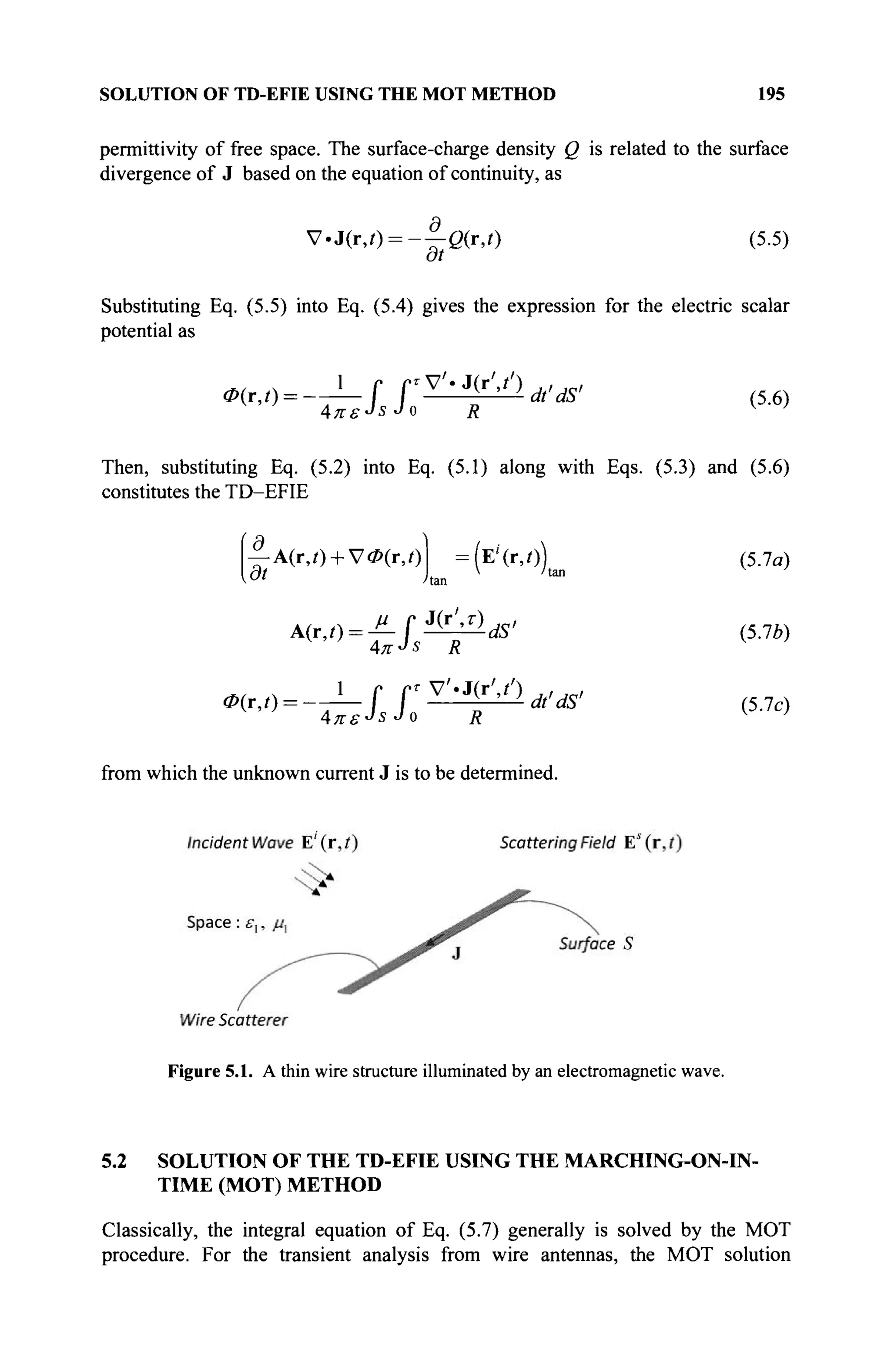
![196 ANALYSIS OF CONDUCTING WIRES IN THE TIME DOMAIN
procedure first was applied by Sayre and Harrington [1]. However, the first
working computer program for transient analysis from wire antennas is contained
in the works of Bennett [2]. Other researchers [3-7] also have applied the MOT
method with much success. The MOT method will not be presented in detail in
this section, as it has been discussed at length for the solution of a general problem
of electromagnetic scattering by 3-D arbitrarily-shaped conducting objects in
section 6.4. In that section, it has been applied to obtain solutions from the TD-
EFIE, TD-MFIE, and TD-CFIE equations. However, we provide a short summary
in this section for completeness to illustrate the basic philosophy of this
methodology.
The solution procedure for MOT starts by factoring the unknown current
J in terms of the scalar temporal and vectorial spatial variables. This can be
written as
J(r,0 = fv„(0f„(r) (5.8)
n=
where N is the number of spatial unknown approximating the spatial variation of
the current on the conducting wire structure.
For finding the numerical solution of the TD-EFIE, the time axis is
divided into segments of equal interval At and a discrete time instant /, is defined
as ti = iAt, where At — /, — ?,_,. Next, assume that all current coefficients are
zero for / < 0, which implies that a causal solution is going to be sought. It is also
assumed that when calculating the unknown coefficients Jn (t) at / = tt, all
coefficients at previous time instants are known. To approximate the time
derivative in the TD-EFIE at the time instant t = ti using the backward finite
difference [8], Eq. (5.7a) can be rewritten as follows:
(A(r,/,)-A(r,// = 1 )+ V Ö ) ( r > / i )
At
:(Е'(г,,г.))(ап (5.9)
or it can be approximated by using the central finite difference [9] at time
t = /,._1/2 to obtain
fA(r,i,.)-A(r,?,·_,) , УФ(г,?,.) + УФ(г,/,_,)1
At
:(E'(r,/,_1/2)) (5.10)
/tan
where central finite difference is used for the time-derivative of the vector
potential and time averaging is used for the scalar potential term.
Equations (5.9) and (5.10) are now solved by applying Galerkin's method
in the MoM context, and hence, the testing function is the same as the expansion
function. By choosing the expansion function fm also as the testing function and
defining the inner product between two functions by Eq. (1.9), Eq. (5.9) becomes](https://image.slidesharecdn.com/timeandfrequencydomainsolutionsofemproblemsusingintegralequationsandahybridmethodologyb-250205130750-568a5ba2/75/Time-and-Frequency-Domain-Solutions-of-EM-Problems-Using-Integral-Equations-and-a-Hybrid-Methodology-B-H-Jung-pdf-217-2048.jpg)
![SOLUTION OF TD-EFIE USING THE MOT METHOD 197
^:(Гт,А(г,г,.)> + (^,УФ(г,0)=(гт ,Е/
(г,0) + ^:(^,А(г,^1 )) (5.11)
and Eq. (5.10) is rewritten as
^(fB1,A(r,//)) + i(fm,VÖ>(r,il.)> = (fm,E'(r,//_1/2))
+^(fm,A(r,?;._1))-^(fm,V0(r,/,_1)) (5.12)
The left-hand sides of Eqs. (5.11) and (5.12) contain the terms at t = tt,and the
right-hand side consists of known quantities, that is, potentials at t = i,_, and the
incident field. Note that both sides of Eq. (5.12) include the scalar potential terms,
and the incident field is considered at the center of the time step. Thus, from either
Eq. (5.11) or Eq. (5.12), a matrix equation can be obtained as follows:
[««»K ('/)] = [&. ft)] (5.13)
The detailed mathematical step to obtain a matrix equation will be described in
section 6.4. The matrix [amn ] is not a function of time, and hence, the inverse of
the matrix needs to be computed only once at the beginning of the computation
step. Finally, by solving Eq. (5.13) at each time step, the time-domain current
induced on the conducting surface may be obtained iteratively.
Some numerical simulations using this procedure will be presented in
section 5.4 and will be compared with results obtained using the MOD solution
and the inverse discrete Fourier transform (IDFT) of a frequency domain solution.
An important disadvantage with this procedure is the possible occurrence
of rapidly growing spurious oscillations at later instants, which is apparently a
result of the accumulation of errors during the calculations. These instabilities
have been touched on by several authors [3,5-7]. Although it may be possible to
eliminate these instabilities, in many cases by a smoothing procedure or by an
implicit implementation as discussed in section 6.4; the accumulation of errors
during calculation puts a limitation on the applicability of this technique [6].
Moreover, with the MOT procedure, the accuracy of the solution [6,7] cannot be
verified easily, and usually there is no error estimation. That is why other
researchers have discussed the use of alternate techniques [10-15], including
iterative methods [6,7] in which the accumulation of errors in time does not take
place. Also, for the iterative methods, the time and space discretizations are
independent of one another, and so one does not have to worry about the
connection between the space and the time discretizations because of Courant-
Friedrich-Levy criteria. There are two iterative methods that have been used,
namely the method of steepest descent [6,7] and the method of conjugate gradients
[7]. However for arbitrarily-shaped structures the iterative methods may be
difficult to apply.](https://image.slidesharecdn.com/timeandfrequencydomainsolutionsofemproblemsusingintegralequationsandahybridmethodologyb-250205130750-568a5ba2/75/Time-and-Frequency-Domain-Solutions-of-EM-Problems-Using-Integral-Equations-and-a-Hybrid-Methodology-B-H-Jung-pdf-218-2048.jpg)

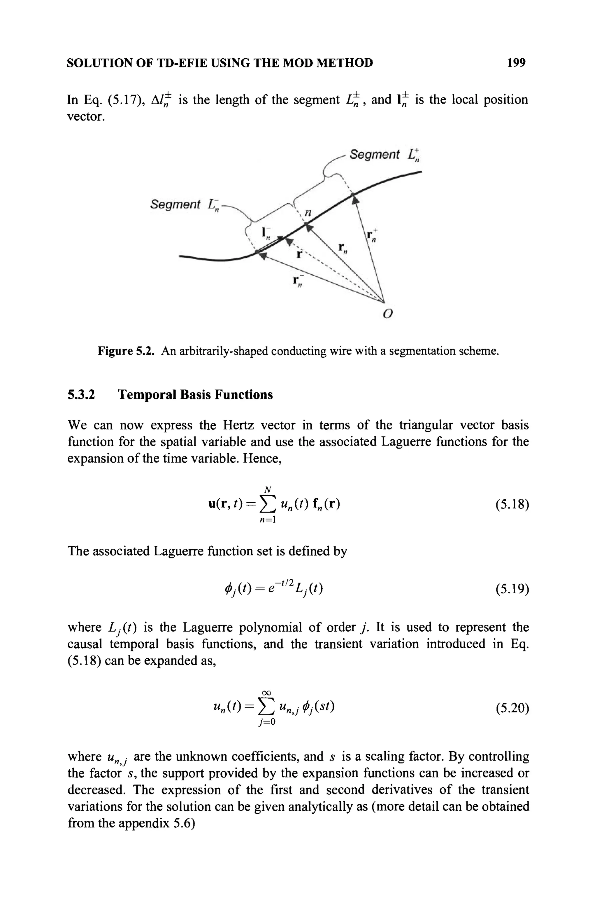
![200 ANALYSIS OF CONDUCTING WIRES IN THE TIME DOMAIN
d °° { 1 J
~l
"' j=0 Δ
4=0
Φ/ist) (5.21α)
d2
7 °° ί 1 ; _ 1
-ju„(t)=s Σ ΤΜ
«,/+ΣΟ'-^ΚΛ
at j = 0 { ч k=0
4>j(st) (5.216)
This assumes that the functions un (0) = 0 and du„ (0)/dt = 0 as the time
response has not started at t = 0 because of causality.
In summary, the following five characteristic properties of the associated
Laguerre functions derived from Laguerre polynomials [16,17] have been used in
this new formulation:
1. Causality: The Laguerre polynomials are defined over 0 < / < + o o for
our applications. Therefore, they are suitable to represent any natural time
domain responses as they are always causal.
2. Recursive computation: The Laguerre polynomials of higher orders can
be generated recursively using the lower orders through a stable
computational process.
3. Orthogonality: With respect to a weighting function, the Laguerre
polynomials are orthogonal with respect to each other. One can construct
a set of orthonormal basis functions, which we call the weighted Laguerre
polynomials or associated Laguerre functions. Physical quantities that are
functions of time can be spanned in terms of these orthonormal basis
functions.
4. Convergence: The associated Laguerre functions decay to zero as time
goes to infinity and therefore the solution does not blow up for late times.
Also, because the associated Laguerre functions form an orthonormal set,
any arbitrary time function can be spanned by these basis functions and
the approximation converges.
5. Separability of the space and time variables: Because of the additivity
property of the weighted Laguerre functions, the spatial and the temporal
variables can be separated completely and the time variable can be
eliminated completely from all computations except the calculation of the
excitation coefficient, which is determined by the excitation waveform
only. This eliminates the interpolation that is necessary to estimate values
of the current or the charge at time instances that do not correspond to a
sampled time instance. Therefore, the values of the current can be
obtained at any time accurately.
Substituting Eqs. (5.18)—(5.21) into Eq. (5.16) results in
4π
2 К со
ΣΣ
1 J
~x
k=0
L
<t>j(sT) f„(r')
dl'](https://image.slidesharecdn.com/timeandfrequencydomainsolutionsofemproblemsusingintegralequationsandahybridmethodologyb-250205130750-568a5ba2/75/Time-and-Frequency-Domain-Solutions-of-EM-Problems-Using-Integral-Equations-and-a-Hybrid-Methodology-B-H-Jung-pdf-221-2048.jpg)
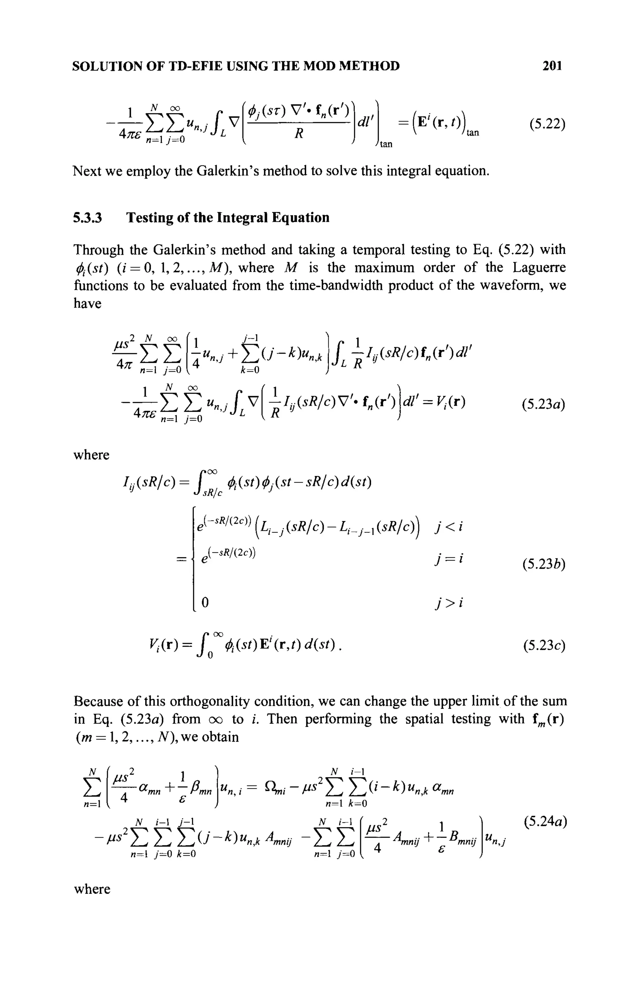
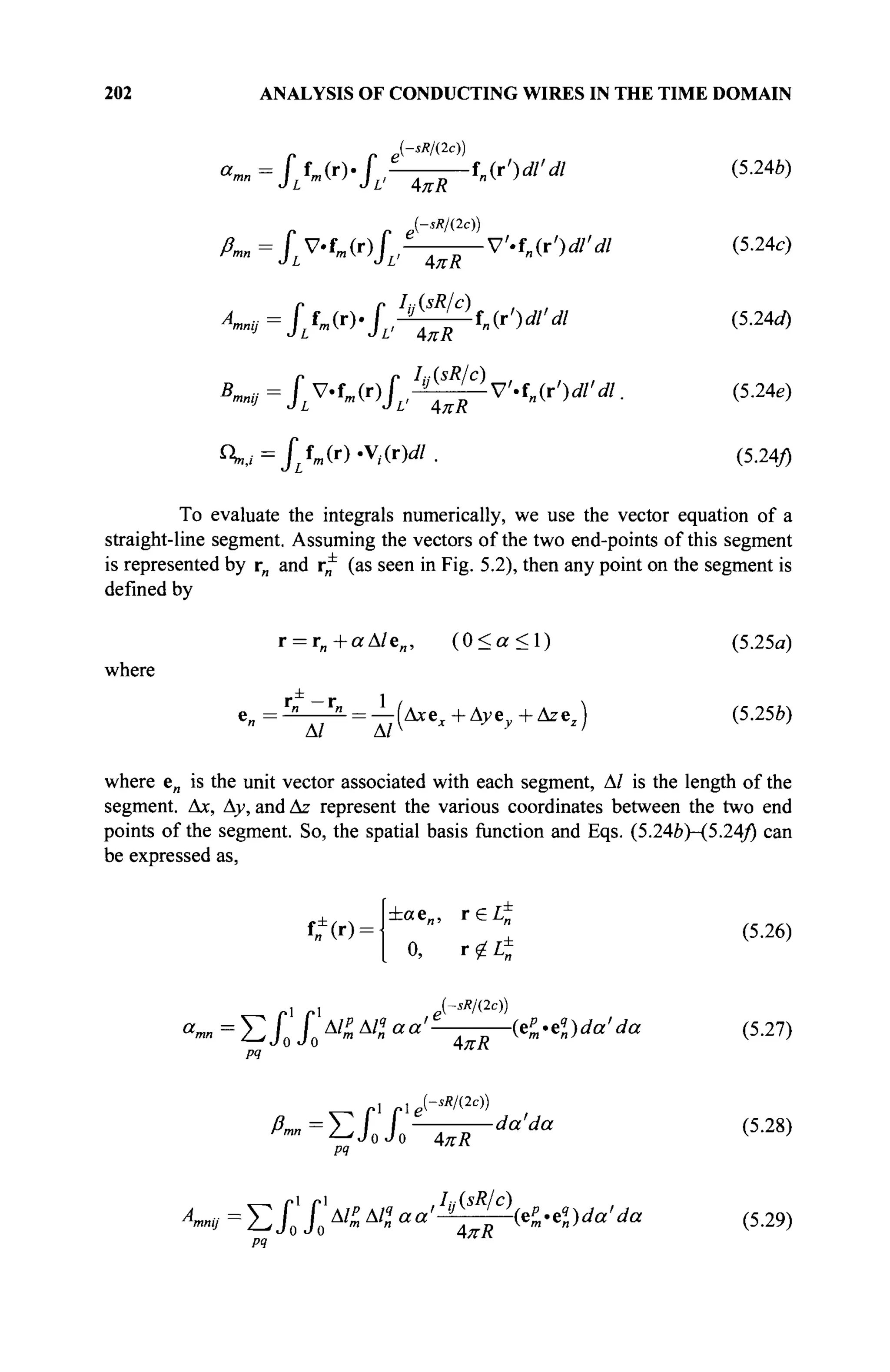
![SOLUTION OF TD-EFIE USING THE MOD METHOD 203
B,mmj ΣΠ' 4πϋ
da'da (5.30)
°м = Σ / ο « ^ « е ^ . / ' ^ Д ^ Е Ч г , ? ) ^ ) ^ (5.31)
where p,q = ±. It should be noted that because the observation point is located on
the surface of the wire, and the current is assumed to be located along the wire axis;
the distance R is always greater than or equal to the radius of the wire, and there
is no singularity in the integrals that one needs to worry about.
Finally, Eq. (5.23a) can be written as
[z
™][«#,,i] = [rB,,i]. » = 1> 2
> 3
> - . M
where
(5.32a)
//S
. mn * Pmn
4 ε
N j -
Ym, i = °гш - Ms2
Σ Σ (i - k) unjk am
n=l 4=0
N i-l j-l N i-l
v«2
]C Σ) Σ 0'-k)unJ[л,«» - Σ Σ
л=1 j=0 k=0 n=l j=0
^-A +-B
л mnij * mnij
(5.32b)
(5.32c)
The matrix element Zmn is not a function of the order of the temporal testing
functions. By solving the matrix equation Eq. (5.32) in a marching-on-in-degree
manner, the electric current is expressed using the relation Eqs. (5,14), (5,18), and
(5.20).
We need to know the finite value of the number of temporal basis
functions, m = , 2, ...,M needed in computing Eq. (5.32). Based on the time-
bandwidth product of the signals that we are trying to approximate, it is possible to
exactly reproduce any arbitrarily-shaped transient waveform of duration Ту and
with a total bandwidth 2B by a set of 2ВТ*+ associated Laguerre functions.
Thus, the minimum number M of the temporal basis functions required to
represent that function becomes [18]
M>2BTf+ (5.33)
Note that in Eq. (5.31), the upper limit of the integral in Ω^ ; can be replaced by
the time sTf instead of infinity.
For analysis of radiation problems, a spatial delta function generator at the
feed node is considered. The inner product given by Eq. (5.24/) w
i m m e
impressed
field and the associated Laguerre functions of order m will be given by](https://image.slidesharecdn.com/timeandfrequencydomainsolutionsofemproblemsusingintegralequationsandahybridmethodologyb-250205130750-568a5ba2/75/Time-and-Frequency-Domain-Solutions-of-EM-Problems-Using-Integral-Equations-and-a-Hybrid-Methodology-B-H-Jung-pdf-224-2048.jpg)
![204 ANALYSIS OF CONDUCTING WIRES IN THE TIME DOMAIN
^=
S7φί{$ί) Vm(
°d{st)
■ (5
·34
)
where vm{t) is the time-dependent source voltage at the common node of the
segment pair m.
5.3.4 Choice of Excitations
Usually, a Gaussian pulse is the most popular excitation for calculating the
transient response of objects. It is considered to be of finite duration in time and
also to be practically band-limited in the frequency domain. A Gaussian pulse is
represented mathematically by
E(r,0 = E0 —π β~γ 2
(5.35α)
Тл]ж
where
r = j(ct-ct0-r.k) (535b)
The parameter с is the velocity of light, к is the unit vector along the direction of
the wave propagation, t is the time variable, T is the width of the pulse and ct0
is the time delay at which the pulse reaches its peak. We use T = 4 lm and ct0 = 6
lm. Both of these quantities are defined in light meters (lm), which is the time
taken by light to traverse 1 m, which is 3.33 ns. This is generally used as the
incident pulse in most time-domain methodologies, as the function needs to be
differentiable. In this chapter, we also consider other types of incident signals like
a triangular-shaped pulse or a rectangular pulse. In this way, response to different
waveshapes, can be evaluated without performing any deconvolution [19].
In this chapter, we use the following triangular pulse for excitation:
E(r,0 =
(t-5) + , 2<t<5
3 '
■i(f-5) + l, 5 < ? < 8 (5.36)
0, others
along with a rectangular pulse of the following shape:
1, 4 < ? < 1 0
E(r,/): (5-37)
0, others
Figure 5.3 presents all three types of signals in the time domain by Figure 5.3(a)
and in the frequency domain by Figure 5.3(b).](https://image.slidesharecdn.com/timeandfrequencydomainsolutionsofemproblemsusingintegralequationsandahybridmethodologyb-250205130750-568a5ba2/75/Time-and-Frequency-Domain-Solutions-of-EM-Problems-Using-Integral-Equations-and-a-Hybrid-Methodology-B-H-Jung-pdf-225-2048.jpg)
![SOLUTION OF TD-EFIE USING THE MOD METHOD 205
(«) (b)
Figure 5.3. Different excitation signals in (a) time domain, and (b) frequency domain.
5.3.5 Treatment of Wire Junctions
Two conditions must be satisfied at a junction. The first one is the enforcement of
the Kirchhoff s current law, which states that the sum of all the currents entering a
junction equals the sum of the currents leaving the junction. The second condition
is that the tangential component of the electric field must be continuous across the
wire surfaces at the junction [19,20]. As shown in Figure 5.4, we replace the actual
junction with a pair of wire segments that are not connected electrically but are
overlapping with each other, as shown in Figure 5.4. Figure 5.4(a) displays the
actual junction of a wire. We treat this junction electromagnetically by considering
it to be two separate wires with overlapping segments, as shown in Figure 5.4(e),
and the total current at the junction will be the sum of all currents at that physical
location.
Next we present some numerical results.
(a) (b)
Figure 5.4. Treatment of a wire junction: (a) Actual junction, (b) Equivalent junction.](https://image.slidesharecdn.com/timeandfrequencydomainsolutionsofemproblemsusingintegralequationsandahybridmethodologyb-250205130750-568a5ba2/75/Time-and-Frequency-Domain-Solutions-of-EM-Problems-Using-Integral-Equations-and-a-Hybrid-Methodology-B-H-Jung-pdf-226-2048.jpg)
![206 ANALYSIS OF CONDUCTING WIRES IN THE TIME DOMAIN
5.4 NUMERICAL EXAMPLES
Analysis of scattering and radiation from wire structures using the MOT and MOD
methods are now discussed. The numerical results obtained by these two methods
are compared with the inverse discrete Fourier transform (IDFT) of the frequency
domain EFIE solution using the same basis functions.
5.4.1 Radiation from a Wire Antenna Solved by the MOT and MOD
Methods
To evaluate the performance of the MOD method in contrast to the MOT
approach, a straight-wire antenna of length / = 1 m located along the z-axis is
considered. The straight-wire antenna is divided into 30 subsections. The radius of
the wire is a — 0.005 m. The excitation is applied at the center of the wire, and
thus, a dipole structure is formed. Figure 5.5 plots the input current at the dipole
antenna using both MOT and the IDFT of a frequency domain solution. An
implicit solution was generated using cAt = 2Rmin, where Λ^,, is the minimum
distance between any two distinct segment centers of the triangular patches. It is
important to note that the solution given by the MOT method using the backward
finite difference has a lower accuracy than when using the central finite
differencing scheme for early times but the latter suffers from late-time
oscillations. The MOT (backward) is based on [21,22] and the MOT (central) is
based on [19,23]. In addition, it is shown that the solution obtained from the MOD
method is stable and has good agreement with the IDFT of the frequency domain
solution.
Figure 5.5. Transient input current at the center of a dipole antenna with a length / = 1 m
and radius a = 0.005 m.](https://image.slidesharecdn.com/timeandfrequencydomainsolutionsofemproblemsusingintegralequationsandahybridmethodologyb-250205130750-568a5ba2/75/Time-and-Frequency-Domain-Solutions-of-EM-Problems-Using-Integral-Equations-and-a-Hybrid-Methodology-B-H-Jung-pdf-227-2048.jpg)
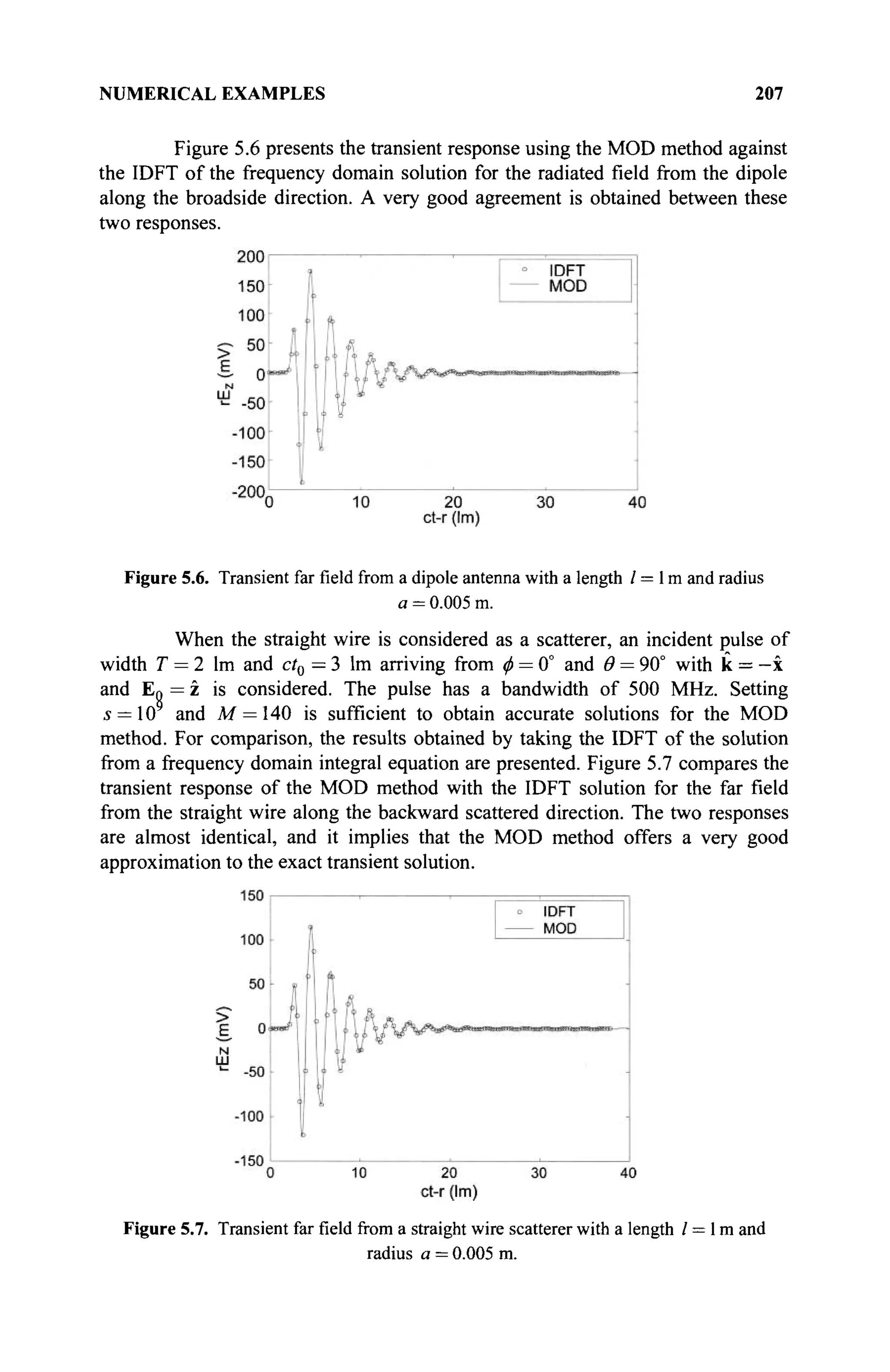
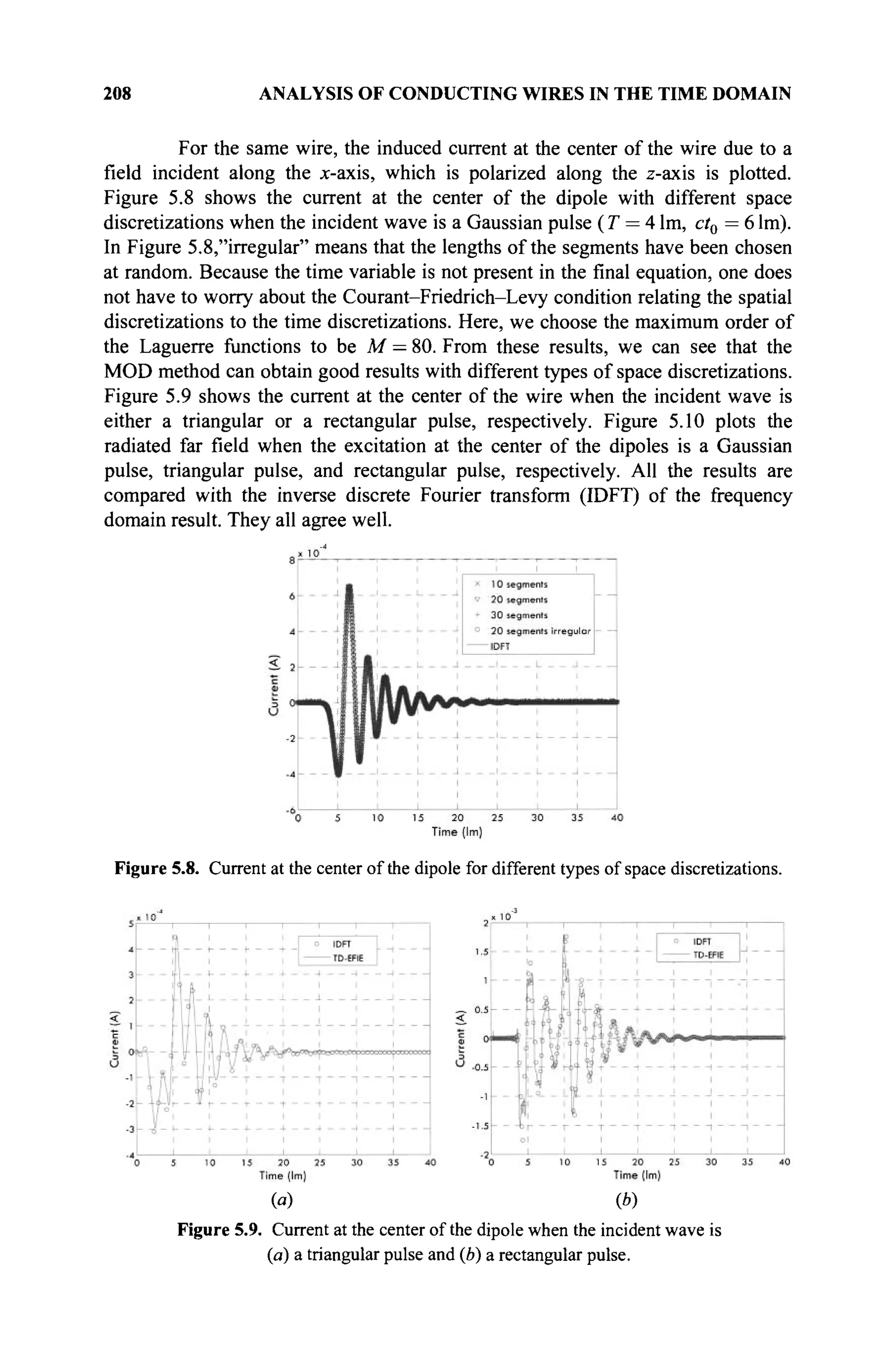
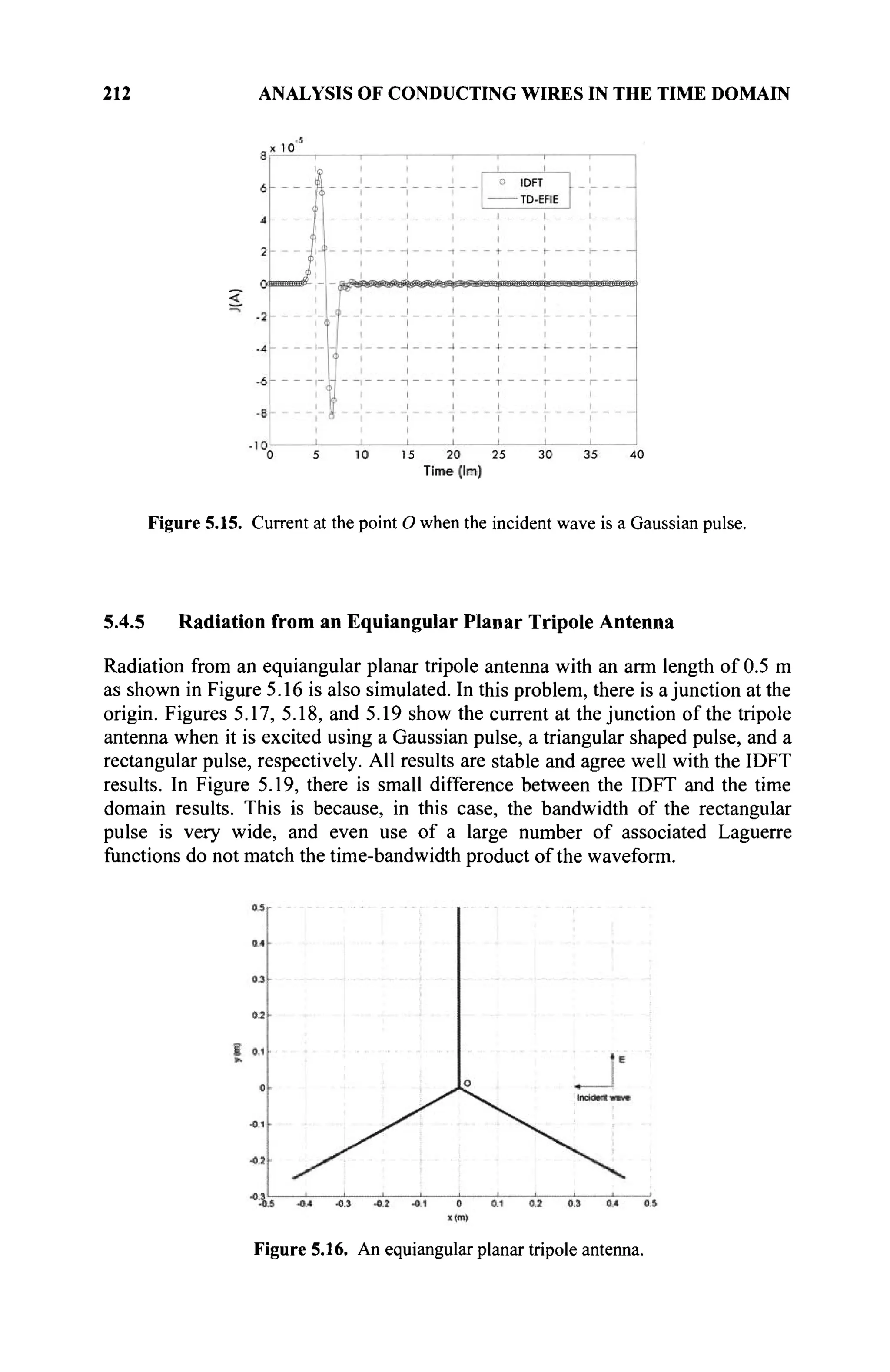
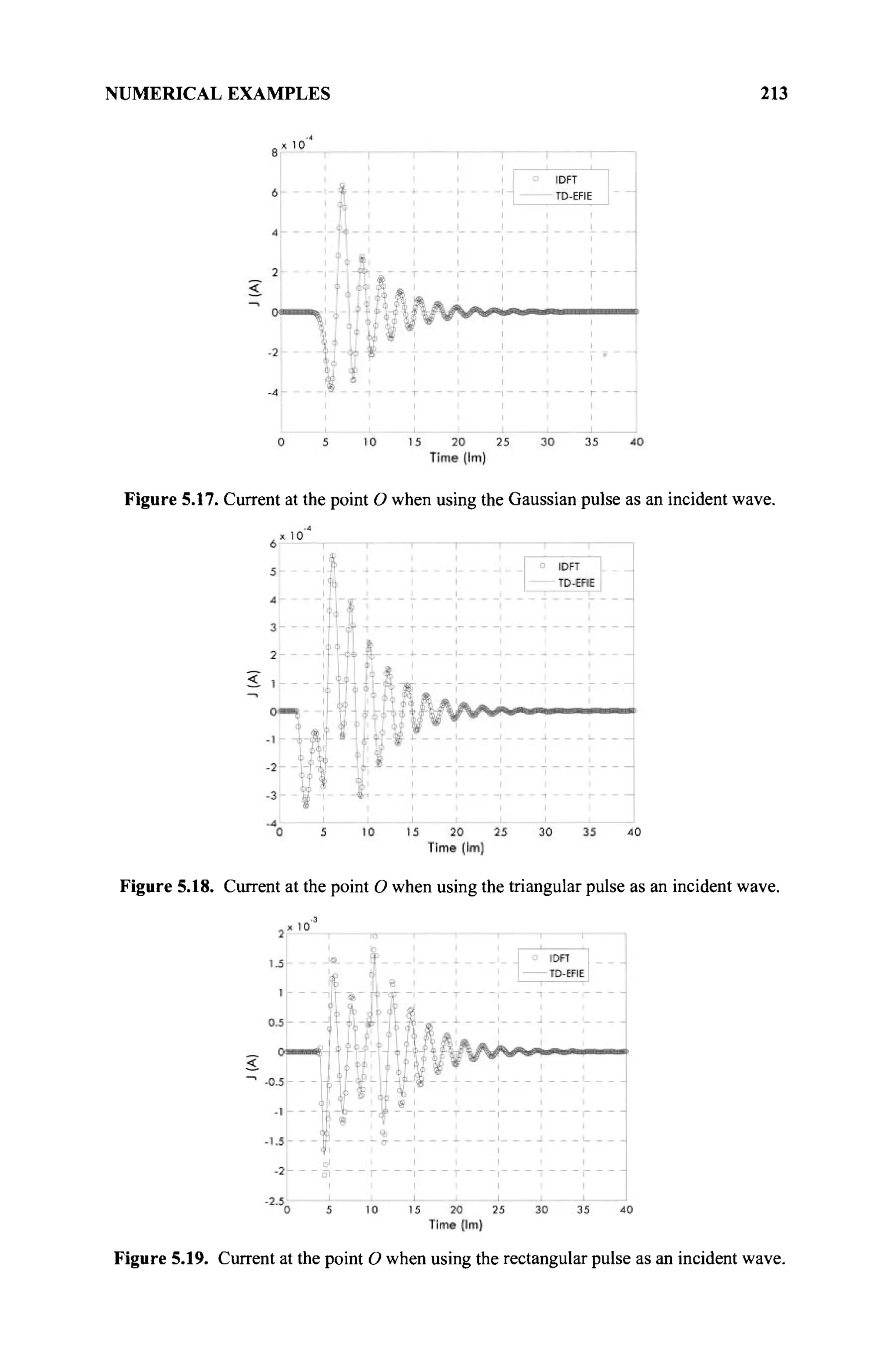
![214 ANALYSIS OF CONDUCTING WIRES IN THE TIME DOMAIN
5.5 CONCLUSION
In this chapter, the procedures to analyze a wire scatterer and antenna by using the
time-domain electric-field integral equation with the MOT and MOD methods
have been presented. For the MOT method, because the size of the time step can
be increased when the implicit scheme is used, the central finite difference
approximates well the derivative of the magnetic vector potential and gives a more
accurate result than the backward finite difference. As such, the marching-on-in-
degree method can be used for solving the time-domain electric field integral
equation for arbitrarily shaped conducting wire structures. The advantage of the
MOD method is to guarantee the late time stability. The temporal derivatives can
also be treated analytically.
This method eliminates the time variable completely from the computations,
and hence, it is a recursion in the order of the Laguerre polynomials. The solution
is thus independent of the time step, and a Courant condition is not necessary. In
addition, any arbitrary waveshape can be used as an excitation, including
discontinuous excitations like a rectangular pulse. Transient currents and far fields
obtained by this method are accurate and stable when compared with the inverse
Fourier transformed data of a frequency domain solution.
5.6 APPENDIX
The definition and properties of Laguerre polynomials are listed in this appendix.
Definition:
Consider the following set of functions [16]:
L
jW> =
^rrj{tlert
)> ° < ' < T O
> 7 = 0,1,2,... (5.A1)
These are the Laguerre polynomials of degree j . They are causal (i.e., they are
defined for t > 0). They can be computed through a stable recursive procedure and
obtained as
A>(0 = 1 (5.A2)
Ll(t) = l-t (5.A3)
Lj{t) = -({2j--t)Lj_x{t)-{j-)Lj_2{t)) j> (5.A4)
The main properties that will be used in the temporal procedures are described
briefly in the following paragraphs.](https://image.slidesharecdn.com/timeandfrequencydomainsolutionsofemproblemsusingintegralequationsandahybridmethodologyb-250205130750-568a5ba2/75/Time-and-Frequency-Domain-Solutions-of-EM-Problems-Using-Integral-Equations-and-a-Hybrid-Methodology-B-H-Jung-pdf-235-2048.jpg)
![APPENDIX 215
Orthogonality:
The associated Laguerre functions are orthogonal as
[1, i = J
Jo°°e-%(/)Ly.(0* = ^ =
^
Laguerre Transform:
A causal time-dependent function f(t) for t > 0 can be expanded as
00
/ C ) = E M W (5.A6)
7=0
where ^.(/) is the associated Laguerre function defined in Eq. (5.19). Based on
the orthogonal property given by Eq. (5.A5), the multiplication of the function
f(t) with φ] (t) and integrating from zero to infinity yields
poo
I №At)dt = ft (5.A7)
The expression in Eq. (5.A7) is called the Laguerre transform.
Derivative:
Using the Laguerre transform, an analytic representation for the time derivative of
the function /(/) can be obtained as
jy^T,mdt
=b+
ΣΛ (5
·Α8
)
Jo dt 2
*=o
where /(0) = 0 is assumed, and $(oo) = 0 is used.
Using the relations (5.A6)-(5.A8), we can expand the derivative of the
function f(t) as
d_
dt j=0
1 ^
fj +
k=0
/ω=Σ 2 ^ + Σ Λ Ф]Ц) (5.А9)
Similarly, the result for the second derivative of the function f(t) is given as](https://image.slidesharecdn.com/timeandfrequencydomainsolutionsofemproblemsusingintegralequationsandahybridmethodologyb-250205130750-568a5ba2/75/Time-and-Frequency-Domain-Solutions-of-EM-Problems-Using-Integral-Equations-and-a-Hybrid-Methodology-B-H-Jung-pdf-236-2048.jpg)
ах (5.A11)
Through a change of variable z = x — y, and substituting the expression of φ^ (t)
given by Eq. (5.19), Eq. (5.A11) yields
Iij{y) = e-y,2
f™ e~Z
Li{z + y)Lj{z)dz (5.A12)
Using the properties of Laguerre polynomials [16; Eqs. (8.971) and (8.974)], we
obtain
m.z + y) = YiLk(z) (A-*O0-A-*-iO0)
k=0
(5.A13)
Substituting Eq. (5.A13) into Eq. (5.A12), one obtains
Iij(y) = e~y/2
Σ (A--*O0-A-*-iO0)£°° e~z
Lk(z)Lj(z)dz (5.A14)
k=0
Because the Laguerre polynomial is defined for z > 0, the lower limit of the
integral in Eq. (5.A14) may be changed from —y to zero. Moreover, Eq. (5.14)
can be computed by using the orthogonal property given by Eq. (5.A5) and yields
the integral of associated Laguerre functions as
J0 Ф-Ах)Ф](*-у)ах
e->/2
(llWO0-£>·_,■_, 00) j<i
0 j>i
(5.A15)
REFERENCES
[1] E. Sayre and R. F. Harrington, "Time domain radiation and scattering by thin
wires," Appl. Sei. Res., Vol. 26, pp. 413-444, 1972.](https://image.slidesharecdn.com/timeandfrequencydomainsolutionsofemproblemsusingintegralequationsandahybridmethodologyb-250205130750-568a5ba2/75/Time-and-Frequency-Domain-Solutions-of-EM-Problems-Using-Integral-Equations-and-a-Hybrid-Methodology-B-H-Jung-pdf-237-2048.jpg)
![REFERENCES 217
[2] С. L. Bennett, A Technique for Computing Approximate Electromagnetic Pulse
Response of Conducting Bodies, Ph.D. Dissertation, Purdue University, Lafayette,
Ind., 1968.
[3] С. L. Bennett and W. L. Weeks, "Transient scattering from conducting cylinders,"
IEEE Tran. Antennas Prop., Vol. 18, pp. 621-633, 1970.
[4] A. M. Auckenthaler and C. L Bennett, "Computer solution of transient time domain
thin-wire antenna problems," IEEE Trans.Micro. Theory and Tech., Vol. 19, pp. 892-
893, 1971.
[5] E. K. Miller and J. A. Landt, "Direct time domain techniques for transient radiation
and scattering from wires," Proc. IEEE, Vol. 68, pp. 1396-1423, 1980.
[6] G. C. Herman, Scattering of Transient Acoustic Waves in Fluids and Solids, Ph.D.
Dissertation, Delft Inst. of Technology, Delft, The Netherlands, 1981.
[7] S. M. Rao, T. K. Sarkar and S. A. Dianat, "The application of the conjugate
gradient method to the solution of transient electromagnetic scattering from thin
wires" Radio Sei., Vol. 19, pp. 1319-1326, 1984.
[8] S. M. Rao and T. K. Sarkar, "Transient analysis of electromagnetic scattering from
wire structures utilizing an implicit time-domain integral-equation technique,"
Micro. Opt. Tech. Lett., Vol. 17, pp. 66-69, 1998.
[9] B. H. Jung and T. K. Sarkar, "Time-domain electric-field integral equation with
central finite difference," Micro .Opt. Tech. Lett, Vol. 31, pp. 429^35, 2001.
[10] S. M. Booker, "Calculation of surface impedance effects on transient antenna
radiation," Radio Sei., Vol. 31, pp. 1663-1669, 1996.
[11] J. F. Callejon, A. R. Bretones, and R. G. Martin, "On the application of parametric
models to the transient analysis of resonant and multiband antennas," IEEE Trans.
Antennas Prop., Vol. 46, pp. 312-317, 1998.
[12] K. Aygun, S. E. Fisher, A. A. Ergin, B. Shanker, and E. Michielssen, "Transient
analysis of multi-element wire antennas mounted on arbitrarily shaped perfectly
conducting bodies," Radio Sei., Vol. 34, pp. 781-796, 1999.
[13] B. H. Jung, T. K. Sarkar, Y. S. Chung, and Z. Ji, "An accurate and stable implicit
solution for transient scattering and radiation from wire structures," Microw. Opt.
Tech. Lett., Vol. 34, pp. 354-359, 2002.
[14] A. G. Tijhuis, P. Zhongqiu, and A. B. Bretones, "Transient excitation of a straight
thin-wire segment: a new look at an old problem," IEEE Trans. Antennas Prop.,
Vol. 40, pp. 1132-1146, 1992.
[15] F. Bost L. Nicolas, and G. Rojat, "A time-domain integral formulation for the
scattering by thin wires," IEEE Trans. Magn., Vol. 36, pp. 868-871, 2000.
[16] A. D. Poularikas, The Transforms and Applications Handbook, IEEE Press, New
York, 1996.
[17] I. S. Gradshteyn and I. M. Ryzhik, Table of Integrals, Series, and Products,
Academic Press, New York, 1980.
[18] Y. S. Chung, T. K. Sarkar, and B. H. Jung, "Solution of a time-domain magnetic-
field integral equation for arbitrarily closed conducting bodies using an
unconditionally stable methodology," Microw. Opti. Tech. Lett., Vol. 35, pp. 493-
499, 2002,
[19] M. R. Zunoubi, N. H. Younan, J. H. Beggs, and С D. Taylor, "FDTD analysis of
linear antennas driven from a discrete impulse excitation," IEEE Trans.
Electromag. Compat., Vol. 39, pp. 247-250, 1997.
[20] T. T. Wu, and R.W. P. King, "The tapered antenna and its application to the
junction problem for thin wires," IEEE Trans. Antennas Prop., Vol. 24, pp. 42^45,
1976.
[21] S. M. Rao and Т. К. Sarkar, "Transient analysis of electromagnetic scattering from
wire structures utilizing an implicit time-domain integral equation technique,"
Micro. Opt. Tech. Lett., Vol. 17, pp. 66-69, 1998.](https://image.slidesharecdn.com/timeandfrequencydomainsolutionsofemproblemsusingintegralequationsandahybridmethodologyb-250205130750-568a5ba2/75/Time-and-Frequency-Domain-Solutions-of-EM-Problems-Using-Integral-Equations-and-a-Hybrid-Methodology-B-H-Jung-pdf-238-2048.jpg)
![218 ANALYSIS OF CONDUCTING WIRES IN THE TIME DOMAIN
[22] S. M. Rao and T. K. Sarkar, "An efficient method to evaluate the time-domain
scattering from arbitrarily shaped conducting bodies," Micro. Opt. Tech. Lett., Vol.
17, pp. 321-325, 1998.
[23] B. H. Jung and T. K. Sarkar, "Time-domain electric-field integral equation with
central finite difference," Micro. Optical Tech. Lett., Vol. 31, pp. 429-435, 2001.](https://image.slidesharecdn.com/timeandfrequencydomainsolutionsofemproblemsusingintegralequationsandahybridmethodologyb-250205130750-568a5ba2/75/Time-and-Frequency-Domain-Solutions-of-EM-Problems-Using-Integral-Equations-and-a-Hybrid-Methodology-B-H-Jung-pdf-239-2048.jpg)
![220 ANALYSIS OF CONDUCTING STRUCTURES IN THE TIME DOMAIN
6.1 INTRODUCTION
The analysis of electromagnetic scattering from arbitrarily shaped conducting
bodies in the time domain has been of considerable interest recently, and many
approaches have been reported in the published literature. Among them, several
approaches have been presented in solving the TDIEs using the triangular patch
RWG basis functions to represent the spatial variations [1-5]. In the expression of
the TD-EFIE, there is a time derivative of the magnetic vector potential. An
explicit solution has been presented by differentiating the TD-EFIE and using
second-order finite difference approximation involving the derivative [1]. But the
computed results become unstable for late times. The late-time oscillations could
be eliminated by taking the average value for the current [2]. However, as the
incident field is also differentiated, this method cannot deal with excitations that
may involve an impulse or a step function. To overcome this problem of the
explicit technique, a backward finite difference scheme is used to approximate the
derivative on the magnetic vector potential [4]. Also, many numerical results using
the explicit method with forward and backward difference schemes to approximate
the derivative have been reported [4-7]. Recently, an implicit scheme has been
proposed to solve two- and three-dimensional scattering problems with improved
late-time stability [8-12]. When the explicit method is used, the time step becomes
very small, and the computed transient response becomes unstable because of the
accumulation of numerical errors at each step, and the overall computation time is
long. When the implicit method is used, a larger time step can be used. But the
numerical error in the approximation for the time derivative using a finite
difference is increased. This implies that the stability and accuracy of a solution
procedure are dependent on the choice of the time step. A central finite difference
methodology has also been used for approximating the time derivative of the TD-
EFIE to improve the stability and the accuracy [13,14]. In addition, numerical
methods based on the TD-MFIE have also been presented for calculating the
transient response from three-dimensional closed conducting bodies [9,15]. It has
been observed that the numerical results obtained using the TD-MFIE is more
stable than those obtained using the TD-EFIE.
It is well known that the numerical solutions obtained using either EFIE
or MFIE for the analysis of closed conducting structures in the frequency domain,
do not provide a unique result when the incident field contains frequencies at
which the structure is resonant. Similar problems are encountered in the time
domain. The methods based on the TD-EFIE and TD-MFIE may produce spurious
solutions in the analysis of closed conducting bodies at frequencies that
correspond to the internal resonance of the structure. One possible way of
obtaining a unique solution is to use the TD-CFIE by linearly combining the TD-
EFIE with TD-MFIE. The TD-CFIE has been applied to the analysis of transient
scattering by two- and three-dimensional bodies [16-18]. This formulation
eliminates the resonance problem and sometimes also the late-time oscillation
encountered in the TD-EFIE and slow varying oscillation of the solution in the
TD-MFIE. However, solutions obtained using the TD-CFIE scheme still may have
an instability problem, and its accuracy is dependent on the size of the time step.](https://image.slidesharecdn.com/timeandfrequencydomainsolutionsofemproblemsusingintegralequationsandahybridmethodologyb-250205130750-568a5ba2/75/Time-and-Frequency-Domain-Solutions-of-EM-Problems-Using-Integral-Equations-and-a-Hybrid-Methodology-B-H-Jung-pdf-241-2048.jpg)
![TIME DOMAIN INTEGRAL EQUATIONS 221
To solve TDIEs, the MOT method has been widely used [5] for many
years. However, a serious drawback of this procedure is that late-time instabilities
occur in the solution in the form of high-frequency oscillations. In Chapter 5, a
method using the Laguerre polynomials as temporal basis functions has been
introduced. The associated Laguerre functions derived from the Laguerre
polynomials are defined only over the interval from zero to infinity and, hence, are
considered to be more suited for the analysis of transient problems, as they
naturally enforce causality [19]. Using the associated Laguerre functions, a set of
orthonormal basis functions is constructed. Transient quantities that are functions
of time can be spanned in terms of these orthogonal basis functions. Because these
temporal basis functions are convergent to zero as time increases to infinity, the
transient response spanned by these basis functions is also expected to be
convergent to zero as time progresses. Using the Galerkin's method, a temporal
testing procedure is introduced. By applying the temporal testing procedure to the
TDIEs, the numerical instabilities can be improved on in contrast to the MOT
method. Another advantage of the MOD procedure over the MOT technique is that
the connection between the spatial and the temporal discretizations related by the
Courant-Friedrich-Levy criteria can be relaxed. In the MOD method, the solution
progresses by increasing the degree of the polynomial involved in the temporal
testing functions. Therefore, the unknown coefficients can be obtained by solving
a matrix equation recursively with a finite number of basis functions. The
minimum number of basis functions is dependent on the product of the time
duration and the frequency bandwidth of the incident wave. In this chapter,
alternative formulations of the MOD method are also presented to solve the TD-
EFIE, TD-MFIE, and TD-CFIE.
In section 6.2, the TD-EFIE, TD-MFIE, and TD-CFIE for analyzing
transient electromagnetic responses from three-dimensional arbitrarily shaped
conducting bodies are presented. Section 6.3 will briefly review the triangular
patch vector function (i.e., the RWG vector functions [20-23]), which will be used
in both the MOT and the MOD methods. The details of generating the matrix
equation using the MOT method will be given in section 6.4, whereas that for the
MOD method and its alternative formulations will be presented in sections 6.5 and
6.6, respectively. Numerical examples illustrating the application of the different
methods are given in section 6.7 followed by some conclusions in section 6.8.
6.2 TIME DOMAIN INTEGRAL EQUATIONS (TDIEs)
6.2.1 Time Domain Electric Field Integral Equation (TD-EFIE)
In this section, the TD-EFIE for the analysis of conducting structures is presented.
Let S denote the surface of a closed or open conducting body illuminated by a
transient electromagnetic wave. Enforcing the boundary condition that the total
tangential electric field is zero on the surface for all time leads to](https://image.slidesharecdn.com/timeandfrequencydomainsolutionsofemproblemsusingintegralequationsandahybridmethodologyb-250205130750-568a5ba2/75/Time-and-Frequency-Domain-Solutions-of-EM-Problems-Using-Integral-Equations-and-a-Hybrid-Methodology-B-H-Jung-pdf-242-2048.jpg)
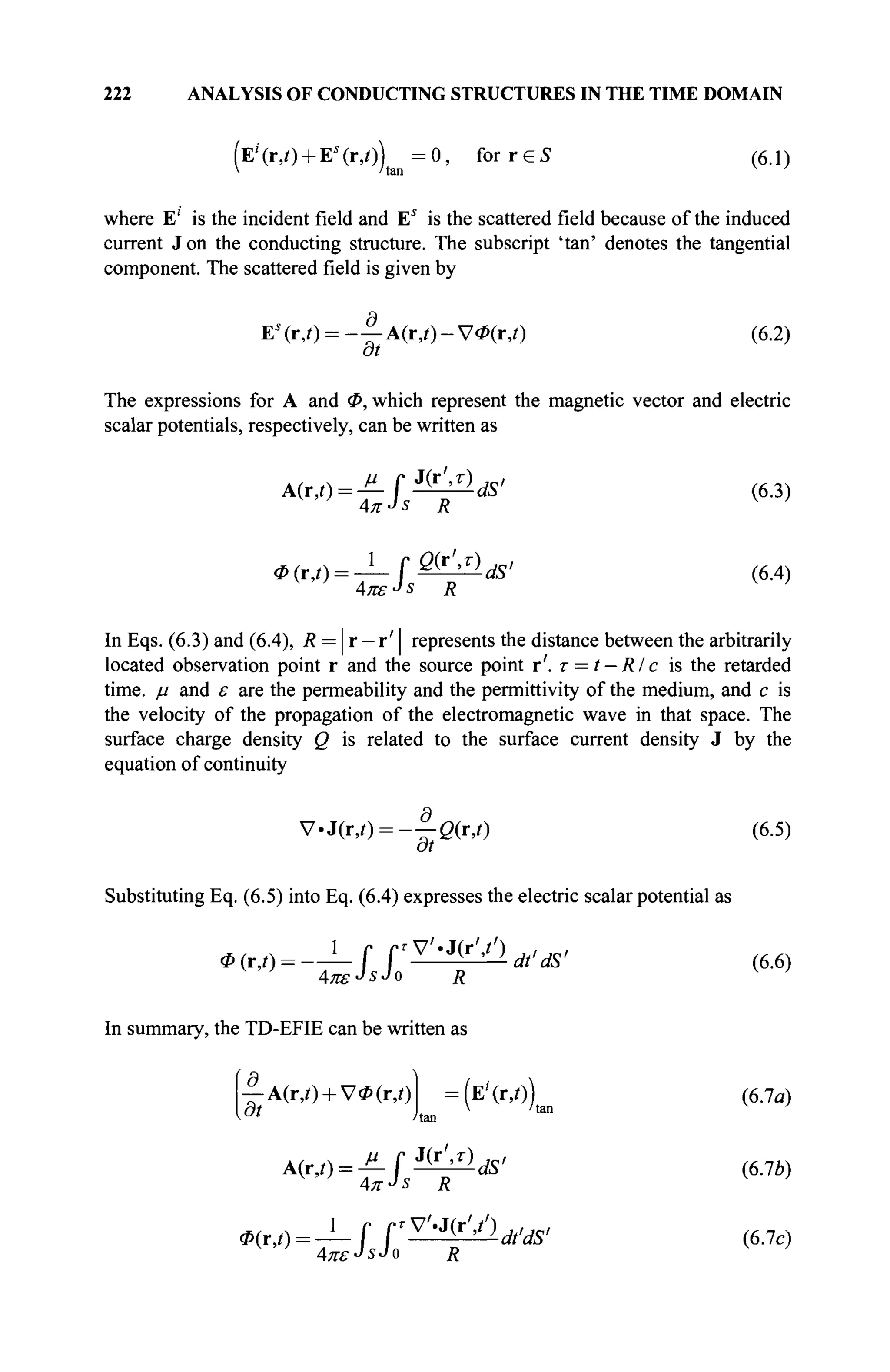
![TIME DOMAIN INTEGRAL EQUATIONS 223
The unknown current J can be obtained from the solution of Eq. (6.7).
6.2.2 Time Domain Magnetic Field Integral Equation (TD-MFIE)
Using the boundary condition for the magnetic field, the TD-MFIE can be
obtained. Let S represent the surface of a closed conducting body illuminated by
a transient electromagnetic plane wave. The TD-MFIE is given by
n x (Η' (r,0 + HJ
(г,/)) = J(r,/), r € S (6.8)
where n represents an outward-directed unit vector normal to the surface S at a
field point. H' is the incident field, and Hs
is the scattered magnetic field caused
by the induced current J. The scattered magnetic field can be written in terms of
the magnetic vector potential as
Hs
(r,i) = - V x A ( r , 0 (6.9)
μ
where A is the magnetic vector potential given by Eq. (6.3). Extracting the
Cauchy principal value from the curl term in Eq. (6.9) yields
n x H s
( r , 0 = ^ + n x - Г V x ^ Ä ' (6.10)
2 4KJS0 R V
'
where S0 denotes the surface S with the singularity at r = r' or R = 0 removed.
Now, by substituting Eq. (6.10) into Eq. (6.8), one obtains
M _ n x l f V x ^ ^ ' - n x H ' f r / ) (6.11)
2 4тг-4 R '
Equation (6.11) is the TD-MFIE, and the unknown current J is to be determined.
6.2.3 Time Domain Combined Field Integral Equation (TD-CFIE)
The time domain CFIE is obtained through a linear combination of the EFIE with
the MFIE [23] through
(1-к-)(-Е*(г,0) +Ä77(j-nxHs
(r,/))
= (l-O(E'(r,0) +m7(nxH'(r,/)) (6.12)](https://image.slidesharecdn.com/timeandfrequencydomainsolutionsofemproblemsusingintegralequationsandahybridmethodologyb-250205130750-568a5ba2/75/Time-and-Frequency-Domain-Solutions-of-EM-Problems-Using-Integral-Equations-and-a-Hybrid-Methodology-B-H-Jung-pdf-244-2048.jpg)
![224 ANALYSIS OF CONDUCTING STRUCTURES IN THE TIME DOMAIN
where к is the parameter of the linear combination, which is between 0 (EFIE)
and 1 (MFIE), and η is the wave impedance of the space. The advantage of the
TD-CFIE over the TD-EFIE and TD-MFIE are that both of the latter equations fail
to give a unique solution when the frequency spectrum of the incident wave
includes internal resonant frequencies of the object. By obtaining a linear
combination of the TD-EFIE and TD-MFIE, the real poles on the frequency axis
are pushed in to the complex frequency plane, thereby eliminating the internal
resonant poles on the cu-axis.
6.3 TRIANGULAR PATCH (RWG) VECTOR BASIS FUNCTION
To numerically solve the TDIEs either by using the MOT or MOD techniques, the
structure of interest is modeled by triangular patches, and the unknown surface
current is approximated by the RWG basis function over the patch, which has been
introduced in the previous chapters [20]. In summary, on the nth edge, the RWG
vector basis function is given by
f„(r) = f„+
(r) + f„-(r) (6.13a)
f,Î(r) = -
- ^ p ±
г е Г е
2a„
0, r ^
(6.136)
where /„ is the length of the edge and a^ is the area of the triangle T*, and p*
is the position vector defined with respect to the free vertex of T^,
6.4 COMPUTED NUMERICAL SOLUTIONS USING THE MOT
The electric current J on the surface of the scatterer may be approximated by
J(r,/) = £y„(0f„(r) (6.14)
«=i
where N represents the number of common edges. By applying the Galerkin's
method and using the same RWG functions as both expansion and the testing, the
operator equation can be transformed into a matrix equation. This matrix equation
is a function of time and can be solved iteratively as the time progresses.](https://image.slidesharecdn.com/timeandfrequencydomainsolutionsofemproblemsusingintegralequationsandahybridmethodologyb-250205130750-568a5ba2/75/Time-and-Frequency-Domain-Solutions-of-EM-Problems-Using-Integral-Equations-and-a-Hybrid-Methodology-B-H-Jung-pdf-245-2048.jpg)
![COMPUTED NUMERICAL SOLUTIONS USING THE MOT 225
6.4.1 Solving the TD-EFIE by the MOT Method
To numerically solve the TD-EFIE given by Eq. (6.7) using the MOT technique,
the time derivative terms are first approximated by finite differences. The time
axis is divided into segments of equal intervals of duration Δ/ with the discrete
time instant defined as i, = iAt, where At = tt — tt_x. The time derivative in Eq.
(6.7) can be approximated by the forward finite difference at t — tt_x as
fA(r,f,.)-A(r, ?,·_,)
At
+ Vi-(r,iM ) :
(ЕЧг,?г_,)) (6.15)
The time derivative in Eq. (6.7) can also be approximated by the backward finite
difference at t = t, as
A(r,i,.)-A(r,i,._,)
At
УФ(г,?,.) = (Ε'(Γ,0) (6.16)
or by using the central finite difference at time / = ti_y2 as
(А(г,/,)-А(г,/м ) , V ^ O + V^r,/,,,))
At
: (E'(IV,_1 / 2 )) (6.17)
'tan
The forward finite difference scheme is usually used in the explicit method for
solving the TD-EFIE [1] whereas the backward finite difference is used for the
explicit and implicit solution procedures [4,8]. The central finite difference was
proposed to improve the accuracy and stability for the implicit solution. In this
scheme, the time averaging is also applied for the scalar potential term when the
central finite difference is used for computing the time derivative associated with
the vector potential. Equations (6.15)—(6.17) can be combined into a unified form
so that a single formulation can implement all these three schemes by
Afc^-Afc/,.,)
At
+ (1 - v)V <Z>(r, ί,. ) + vV Ф(г, ί,._! )
= ( Е ' ( г , ^ ) )
V 'tan
(6.18)
where v — 1 is for the forward, v = 0 for the backward, and v = 1 / 2 for the
central finite difference approximation.
Equation (6.18) is now solved by applying the Galerkin's method. By
choosing the expansion functions fm as the testing functions and defining the
inner product by Eq. (1.9), one obtains](https://image.slidesharecdn.com/timeandfrequencydomainsolutionsofemproblemsusingintegralequationsandahybridmethodologyb-250205130750-568a5ba2/75/Time-and-Frequency-Domain-Solutions-of-EM-Problems-Using-Integral-Equations-and-a-Hybrid-Methodology-B-H-Jung-pdf-246-2048.jpg)
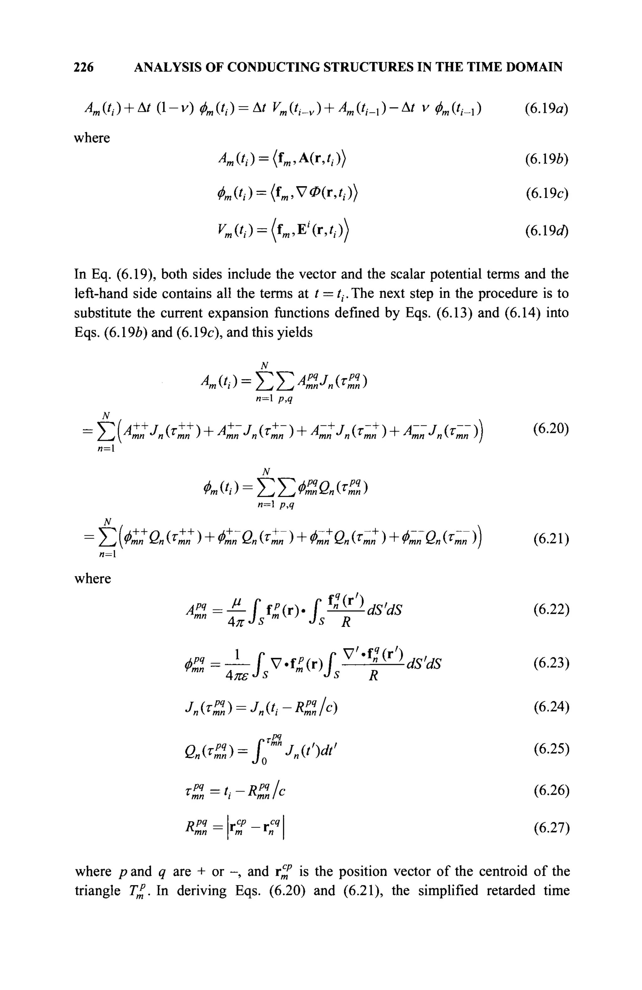
![COMPUTED NUMERICAL SOLUTIONS USING THE MOT 227
ti: — RI c « t,,— R^l I c is assumed and R™n represents the distance between the
centers of testing triangle T£ and source triangle Tq
. This assumption implies that
the current distribution on a triangular patch does not vary appreciably with time.
If the integrals involving the unprimed variables in Eqs. (6.22) and (6.23)
are evaluated by approximating the integrand by their respective values at the
centroids of the testing triangle, Eqs. (6.22) and (6.23) become
4*-L f A-as'
кРЧ lml
-
rmn
tea? JT
* Rt
(6.28)
(6.29)
where R% = r^f — r ' , /„ is the length of the nonboundary edge and aq
n is the area
of the source triangle Tq
. Vectors p4
n are the position vector defined with respect
to the free vertices of Г/. lm is the length of the edge and αζ is the area of the
testing triangle T%. The average charge density is given by the value of p at the
centroid of the triangular patch r^f (i.e., ρ^ = ρ ^ / « „ ) · The integrals in Eqs.
(6.28) and (6.29) may be computed by the methods described in [21].
Finally, Eq. (6.19c/) can be computed by approximating the testing
integral by the value at the centroid of the testing triangle as
ymifi) = TiV^tt)=V+(ti) + V-{ti) ( 6 3 0 )
P
V^(ti) = Jsf^r).Ei
(r,ti)dS^^'Ei
(C,ti) (6.31)
where p can be either + or -. Furthermore, when R^n > сAt or
O-i < r
™ ^ 0 ' w n e r e
0 — *'-i ' ш е c u r r e n t
coefficients Jn (т^ч
„ ) in Eq. (6.24) and
the integration of the current coefficient Qn(T^q
n) in Eq. (6.25) can be rewritten as
Jn^Z) = ( ΐ - ^ μ „ ( 0 - ι ) + ^ « ( 0 ) (6-32)
Qn(T^) = At^2jll(tk) + ^ l + 2ô-S2
)J„(tj_i) + ^-S2
Jl,(tJ) (6.33)
k=o l z
where](https://image.slidesharecdn.com/timeandfrequencydomainsolutionsofemproblemsusingintegralequationsandahybridmethodologyb-250205130750-568a5ba2/75/Time-and-Frequency-Domain-Solutions-of-EM-Problems-Using-Integral-Equations-and-a-Hybrid-Methodology-B-H-Jung-pdf-248-2048.jpg)
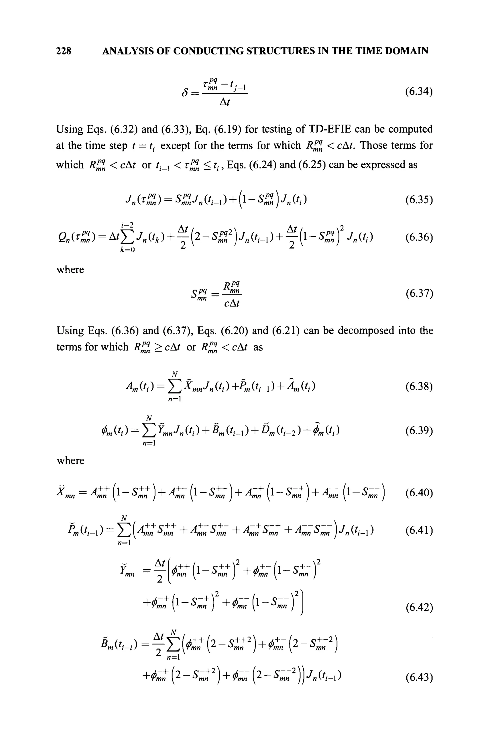
![COMPUTED NUMERICAL SOLUTIONS USING THE MOT 229
Dm ('/-2 ) = Δ ' Σ ( < C + Φ™ + Φ™ + Фшп ) Σ J
n ('* ) (6.44)
In Eqs. (6.38)-(6.44), the symbol _ on top of the elements is used to indicate the
elements for which R^n < сAt and the symbol „ is for elements when
R™ >cAt. The terms Дд/,·) and фт(^) in Eqs. (6.38) and (6.39) for which
R™n > сAt, are of the same form as in Eqs. (6.22) and (6.23). A matrix çquation is
obtained by substituting Eqs. (6.38) and (6.39) into Eq. (6.19) as
[«1][лс,·: (6.45α)
where
E
<n=^mn+^t{-v)Ymn (6.45b)
?E
ßmn = ^tVm (/,_„ ) + A„ (/,_, ) - А1уфт (/,_, )
-(Â^ + PJt^-Atil-v^l^ + B^t^ + D^t^)) (6
-45c
)
Note that when v = 1 for the forward difference case, the terms related to the
scalar potential Ymn in Eq. (6.45b) and фт{!,) + ВтЦ,_{) + Ё>тЦ,_2) in Eq. (6.45c)
vanish and do not contribute to a^n and ß%, respectively. When v = 0 for the
backward difference approximation, the scalar potential term in Eq. (6.45c),
фт (/,·_! ), does not contribute to β^. However, when v = 1 / 2 for the central
difference case, the scalar potential contributes to both the matrices a^n and
ßm· And the incident field is considered at the midpoint of each time step.
Matrix a^n is not a function of time, and hence, the inverse of the matrix needs
to be computed only once at the beginning of the computation.
6.4.2 Solving the TD-MFIE by the MOT Method
In this section, the procedures for solving the TD-MFIE given by Eq. (6.11) using
explicit or implicit schemes are presented. The TD-MFIE is valid only for closed
scatterers. The surface of the closed structure to be analyzed is modeled by planar
triangular patches, and the unknown surface current J is approximated by Eq.
(6.14) in terms of the RWG basis function given by Eq. (6.13).
By applying Galerkin's method, the expansion functions fm are also
chosen to be the testing functions. Applying the testing procedure to Eq. (6.11)
results in](https://image.slidesharecdn.com/timeandfrequencydomainsolutionsofemproblemsusingintegralequationsandahybridmethodologyb-250205130750-568a5ba2/75/Time-and-Frequency-Domain-Solutions-of-EM-Problems-Using-Integral-Equations-and-a-Hybrid-Methodology-B-H-Jung-pdf-250-2048.jpg)
![230 ANALYSIS OF CONDUCTING STRUCTURES IN THE TIME DOMAIN
Cm(t) = rm(t) + Bm(t) (6.46a)
where
Cm(t) = (im,^^j (6.46ft)
^ ( 0 = (fm ,nxH4r,0) (6.46c)
Bm(0 = ( f . . - x ^ / 5 b V x i ^ ^ (6A6ä)
6.4.2.1 Explicit Solution. For solving Eq. (6.46) using the explicit scheme, the
RWG basis functions defined in Eq. (6.17) is substituted into Eq. (6.46ft), and then
Cm(t) becomes
JV
Ст(0 = £С
™Л(0 (6-47«)
n=
where
^■mn =
2-j ^mn =
^mn + ^ ш ' ^mn + ^mn (6 Alb)
PA
СР
1={КЛ1) (6.47с)
where p and q are + or — . Applying Eq. (6.17ft), the inner product integral C^n
defined in Eq. (6.47c) can be further expanded analytically, and the result is given
by [22]
m n
mn
8 a?
3 | CP2
1 ,, ,- ,
rP -I r -4- r
4I m
I I?'' ' ' '
-C-(r
ml+r
„l) +r
ml·»·«! J (6.48)
where rml, rm2, and rm3 are the position vectors of the three vertices of the
triangle T£, and r^f is the centroid of triangle Τζ. rml and гя1 are the position
vectors of the free vertex of the triangle T£ and Τ^, respectively. Note that if the
field point does not lie on the triangle, Tq
( i.e. r ^ 7jf ) then the result is
C£l = 0. This is evident from the definition of the expansion functions in Eq.
(6.17ft).
Next, performing a similar expansion procedure for the term /m(t)
involving an inner product in Eq. (6.46c) results in](https://image.slidesharecdn.com/timeandfrequencydomainsolutionsofemproblemsusingintegralequationsandahybridmethodologyb-250205130750-568a5ba2/75/Time-and-Frequency-Domain-Solutions-of-EM-Problems-Using-Integral-Equations-and-a-Hybrid-Methodology-B-H-Jung-pdf-251-2048.jpg)
![COMPUTED NUMERICAL SOLUTIONS USING THE MOT 231
where
Ут(*) = ^2Гт=Г^+Гт
2a*L J
T&
(6.49a)
(6.49Й)
In Eq. (6.496), the integral is evaluated by approximating the integrand by the
value at the centroid of the testing triangle T£.
Finally, consider the inner product term Bm(t) in Eq. (6A6d). Using a
vector identity, the curl term inside the integral is given by [3]
VxJ(r',T) = ldJ(r',T)yR J(r',r)xR
R с дт R R2
where R is a unit vector along the direction of r - r'. Thus,
(6.50)
,J(r',r)
AKJ
S0 R 4π
1 , 8^г)хК^ г J M x R ^
cJs0 дт R Js0 R2
(6.51)
Now, by substituting Eq. (6.51) into Eq. (6.46a*), one obtains
ß
^=iJ>nx
cJ
s0 дт R Js0 R2 dS (6.52)
Substituting the current expansion given by Eq. (6.14) into Eq. (6.52) and
approximating the value of the retarded time as
T = t-
R Rpq
С С
where R^n = r^" — r^4
is the distance between the centroids of triangle T£ and
T%, one obtains
Kit)=ΣΣΒ
%=ΣΚ«+
+в
™ +в
™ +Кп)
п= p,q и=1
(6.53а)
where](https://image.slidesharecdn.com/timeandfrequencydomainsolutionsofemproblemsusingintegralequationsandahybridmethodologyb-250205130750-568a5ba2/75/Time-and-Frequency-Domain-Solutions-of-EM-Problems-Using-Integral-Equations-and-a-Hybrid-Methodology-B-H-Jung-pdf-252-2048.jpg)
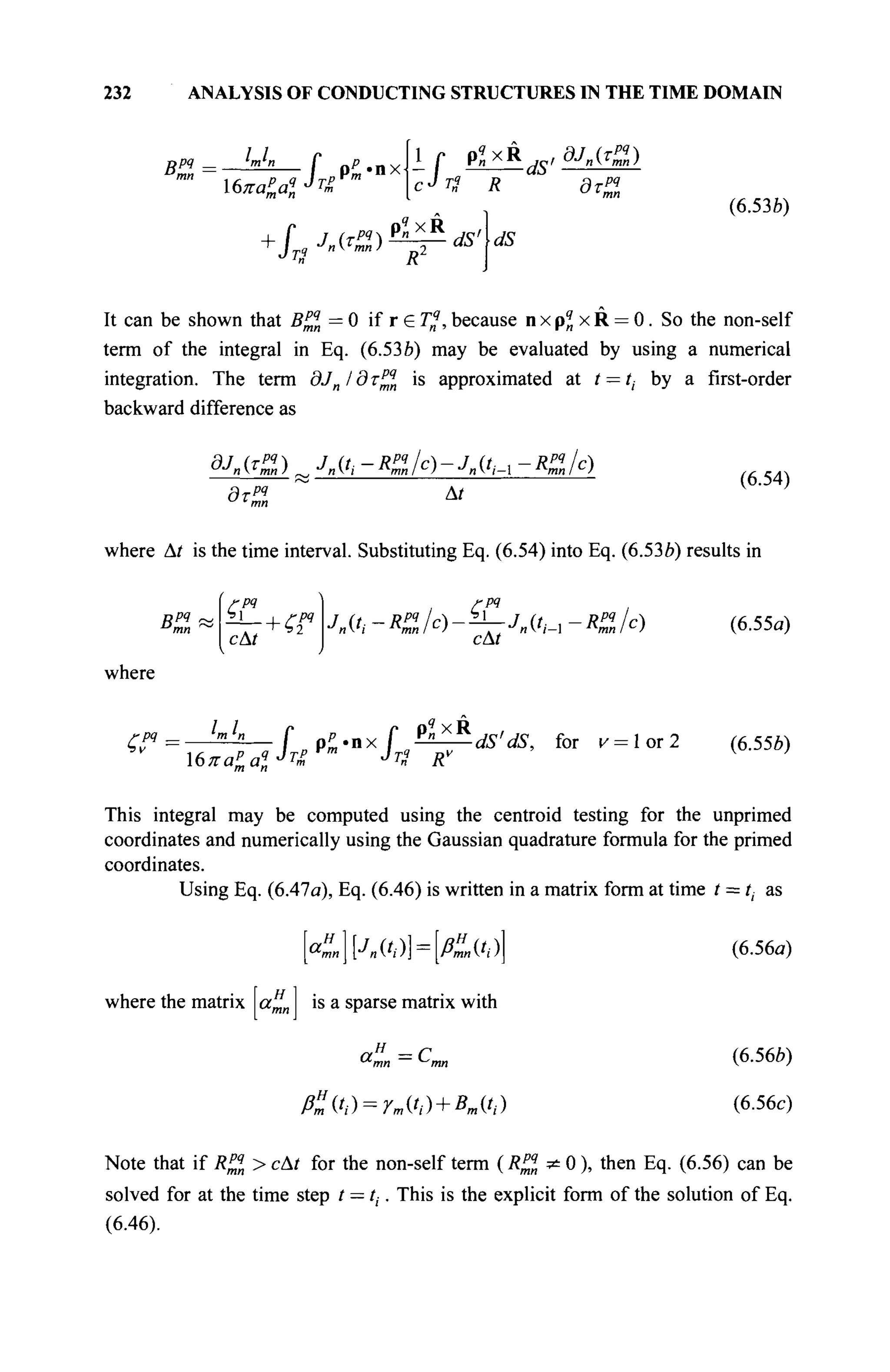
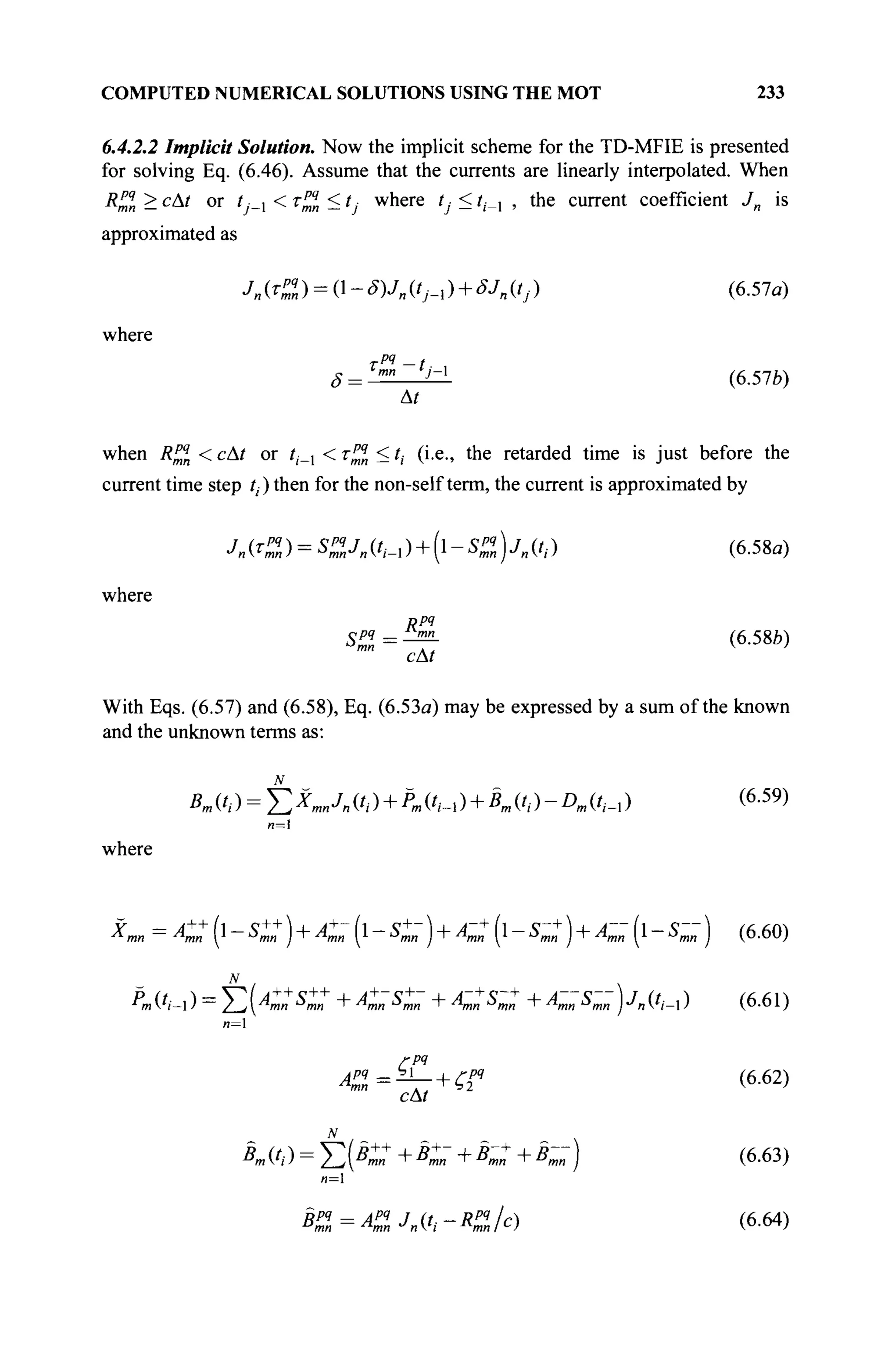
![234 ANALYSIS OF CONDUCTING STRUCTURES IN THE TIME DOMAIN
t
"1
D
m (',-ι ) = Σ (D
™ +D
™ +D
™ +D
™ ) (6.65)
DZ=^-Jn{t^-R%c). (6.66)
In Eqs. (6.59)-(6.64), Jfmn and Pm, which are marked with the symbol ^ on the
top, are obtained by collecting the terms that satisfy the condition Rj* < сAt and
Bm, which is marked with the symbol _ on the top, are obtained by collecting the
terms that satisfy the condition R™n > с At.
Finally, by substituting Eqs. (6.47) and (6.59) into Eq. (6.46), a matrix
equation is obtained as
[«™][Л(',·)] = [/&(',)] (6.67«)
where
aH
mn=Cmn-Xmn (6.67Ô)
ßm (t,) = Ym ift) + К C^-l ) + Кft) + Dm (?,_, ) (6.67c)
Eq. (6.67) constitutes the implicit solution of the TD-MFIE.
6.4.3 Solving the TD-CFIE by the MOT Method
Because the TD-CFIE is obtained by a linear combination of the EFIE and MFIE,
the solution of the CFIE can thus be obtained directly by a combination of the
solutions for the EFIE of Eq. (6.45) and the explicit solution of MFIE of Eq. (6.56)
or the implicit solution of MFIE of Eq. (6.57). A matrix equation can be obtained
directly by combining Eqs. (6.56) and (6.67) as
[«1][Л ('/)] = [/&(',)] (6.68α)
where
«™ = 0 - « « I + κηαί, (6-68Й)
ßm ft ) = (1 - K)ßE
mft) + κηβ» ft ) (6.68c)
6.5 COMPUTED NUMERICAL SOLUTIONS BY THE MOD
The TDIEs obtained for arbitrarily shaped 3-D conducting structures can
alternatively be solved by using the MOD method, which has been outlined in](https://image.slidesharecdn.com/timeandfrequencydomainsolutionsofemproblemsusingintegralequationsandahybridmethodologyb-250205130750-568a5ba2/75/Time-and-Frequency-Domain-Solutions-of-EM-Problems-Using-Integral-Equations-and-a-Hybrid-Methodology-B-H-Jung-pdf-255-2048.jpg)
![COMPUTED NUMERICAL SOLUTIONS BY THE MOD 235
Chapter 5 for the analysis of a conducting wire. The computational procedure for
analysis of 3-D conducting objects is similar to that for a conducting wire. In this
section, the procedures for solving the TD-EFIE, TD-MFIE, and TD-CFIE using
the MOD method will be described. The first step in the MOD and the MOT
methods are similar. The surface of the structure to be analyzed is modeled by
planar triangular patches. The MOD procedures are based on the Galerkin's
method which involves separate spatial and temporal testing procedures.
Piecewise triangle basis functions are used for spatial expansion and testing,
whereas the time-domain variation is approximated and tested by a temporal basis
function set derived from the associated Laguerre functions. Also, a new Hertz
vector u(r, t) is introduced in the MOD method for operational convenience; in
particular it is good for handling the time integral in the TD-EFIE analytically.
The current is related to the Hertz vector by
J(r,0 = -J-u(iy) (6.69)
at
and the relation between this Hertz vector and the electric charge density Q(r, t)
is given through
ß(r,0 = - V - u ( r , 0 (6.70)
Using the RWG basis functions of Eq. (6.13), the Hertz vector is spatially
expanded as
N
u(r,/) = £>«(') W (6.71)
n=l
Next, the TDIEs are tested with the same RWG function. Then, the temporal
variation of the Hertz vector is expanded in terms of an orthonormal associated
Laguerre functions set <j)Àt), which is derived from the Laguerre polynomials
through the representation [19]
ф^) = е-,
%«) (6.72)
where Lj (t) is the Laguerre polynomial of degree j . By using this basis function,
the transient coefficient for the Hertz vector introduced in Eq. (6.71) is expanded
as
oo
"»(0 = Е % ^ Й
) (6.73)](https://image.slidesharecdn.com/timeandfrequencydomainsolutionsofemproblemsusingintegralequationsandahybridmethodologyb-250205130750-568a5ba2/75/Time-and-Frequency-Domain-Solutions-of-EM-Problems-Using-Integral-Equations-and-a-Hybrid-Methodology-B-H-Jung-pdf-256-2048.jpg)
![236 ANALYSIS OF CONDUCTING STRUCTURES IN THE TIME DOMAIN
where 5 is a scaling factor. By controlling this factor s, the support provided by
the expansion can be increased or decreased. Applying the derivative property for
the associated Laguerre functions given in the appendix of Chapter 5, the first and
second derivatives of the transient coefficient un(t) are obtained as
d °° ί 1 ■/_1
" ' j=0 { Z
k=0
ФМ) (6.74)
df 7=0
y-i
—jun(t) = s2
^2 -ип]+^и-к)ипк
k=0
Ф№) (6.75)
The TDIEs are then tested with the temporal basis function ф} (t). By substituting
Eqs. (6.73), (6.74), and (6.75) in the temporal testing of the TDIEs, the unknown is
expressed in terms of a matrix equation that can be solved iteratively as the degree
of the polynomial increases from a small to a large value.
6.5.1 Solving the TD-EFIE by the MOD Method
The TD-EFIE of Eq. (6.7) can be solved by applying the Galerkin's method. Using
the RWG vector functions fm (r) for both spatial expansion and testing, Eq. (6.7)
yields
(r), |-A(r,0) + (fm(r), УФ(г,0) = (fm(r), E'(r,0) (6.76)
Substitute Eqs. (6.69), (6.70), and (6.71) into the first term of Eq. (6.76). Also, use
Eq. (6.3) for the magnetic vector potential A to yield
Θ f
> ' ) M,.
fm(r), - A(r,0) = Σ ^ J > r ) ' / ^ ω ψ dS'dS (6.77)
By assuming that the unknown transient quantity does not change appreciably
within a triangle, one can obtain
r = t-
R
τη
=t-
Rpq
mn npq _ _cp _ r < 4
' mn m n
(6.78)
where p and q are + or -, and rc
m is the position vector for the centroid of the
triangle T^. Eq. (6.77) can be rewritten as](https://image.slidesharecdn.com/timeandfrequencydomainsolutionsofemproblemsusingintegralequationsandahybridmethodologyb-250205130750-568a5ba2/75/Time-and-Frequency-Domain-Solutions-of-EM-Problems-Using-Integral-Equations-and-a-Hybrid-Methodology-B-H-Jung-pdf-257-2048.jpg)
![COMPUTED NUMERICAL SOLUTIONS BY THE MOD 237
where
&=±№ν·ί?ψ<Β·<*
(6.79α)
(6.79*)
Next, consider the testing of the gradient of the scalar potential <Z>(r,i)in the
second term of Eq. (6.76). Using the vector identity V*^A = А· Уф + фУ»А and
the property of the spatial basis function [20], this term can be written as
(fm (г), УФ (r, 0} = -Js V · f
m (г) Ф (r,0 dS
dS
(6.80)
Based on the assumption defined in Eq. (6.78), Eq. (6.80) can be written as
N opq
(fm(r), УФ(г,;)) = Σ Σ - «-(О
n=l PA
where
V'«f?
(r')
B% = — f V- f£(r) Г V Л ;
«fi"dS
Similarly, the term in the right side of Eq. (6.76) can be expressed as
(fm (r),E''(iy))=^(0
rçf(/) = /fw(r).E'(r,0dS
(6.81α)
(6.816)
where
(6.82α)
(6.826)
Finally, substituting Eqs. (6.79), (6.81), and (6.82) into Eq. (6.76) one finally
obtains the result as
ΣΣ
n=l p,q
where
dt ε
ASi^Ifi^.fß^dS'dS
v*{t)
s R
(6.83α)
(6.836)](https://image.slidesharecdn.com/timeandfrequencydomainsolutionsofemproblemsusingintegralequationsandahybridmethodologyb-250205130750-568a5ba2/75/Time-and-Frequency-Domain-Solutions-of-EM-Problems-Using-Integral-Equations-and-a-Hybrid-Methodology-B-H-Jung-pdf-258-2048.jpg)
![238 ANALYSIS OF CONDUCTING STRUCTURES IN THE TIME DOMAIN
BZ = — Г ν · f^(r) Г v / , f
"( r / )
ds'ds
m
" 4KJs m
'Js R
V*(t) = ffm(r).Ei
(r,t)dS
(6.83c)
(6.83</)
The detailed evaluations of these integrals are described in [20] and [21]. Then the
temporal expansion and testing procedures are now carried out using the
associated Laguerre functions. The terms ип(трч
„) and d2
un(Tpq
n)/dt2
in Eq.
(6.83a) are substituted by Eqs. (6.73) and (6.75) and the temporal testing with
Φι (st) is taken, resulting in
ΣΣΣ
w—1 p,q j=Q
7РЯ
' 2
. Mл
тп +
4 ε
У-1
/ + S V C E ( J 4
) ^
k=0
hj^Kilc)
(6.84a)
where
In
yisRZ/c) = Г , fast) ф№-5Я%/с) d(st) (6.846)
(6.84c)
The integral in Eq. (6.84b) can be computed by applying the integral property of
the associated Laguerre functions given in the appendix of Chapter 5. Note that 1ц
= 0 when j > i. Therefore, the upper limit of the third summation symbol in Eq.
(6.84a) can be written as i instead of oo. Moving those terms including и for
j < i, which are known, to the right-hand side of Eq. (6.84a) can result in
ΣΣ
n=l PA
(
s2
Bpq
4 ε
«nJ^R^/c)
N i-l (
s2
Bpq
4 ε
UnjhjWZlc)
<*-ΣΣΣ
n= p,q j—0
-Σ Σ E*V4£ Σ O"-*)«*,* ¥<«A)
л=1 p,q j=0 k=0
(6.85)
When Eq. (6.85), is rewritten, we obtain](https://image.slidesharecdn.com/timeandfrequencydomainsolutionsofemproblemsusingintegralequationsandahybridmethodologyb-250205130750-568a5ba2/75/Time-and-Frequency-Domain-Solutions-of-EM-Problems-Using-Integral-Equations-and-a-Hybrid-Methodology-B-H-Jung-pdf-259-2048.jpg)
![COMPUTED NUMERICAL SOLUTIONS BY THE MOD 239
f a
£
„ . = vE
.+pE
.
where
a„ =Σ
/>.<?
-μΑΖ^—
Bpq
ε
**%,/&))
(6.86a)
(6.86b)
n= p,q
s Врч
s
μΑη+Ën»
4 ε
i-
Y^u^I^sRM/c)
j=o
7=0 *=0
(6.86c)
In deriving Eq. (6.86), the property of the integral related to the temporal basis
function given by Eq. (5.A15) is used. The term Iä(sRpq
n/c) can be represented by
an exponential term because of /,·,· (>>) = e~yl2
for j = i. Finally, Eq. (6.86) can
be written into a matrix form as
^mn u
n,i rE
] (6.87)
where γΕ
,· =VE
i+PE
i and / = 0,1, ...,oo. It is important to note that [aE
n] is
not a function of the degree of the temporal testing function. After the temporal
testing procedure, the unknown coefficients un (J) can be obtained by solving Eq.
(6.87) by increasing the degree of the temporal testing functions.
6.5.2 Solving the TD-MFIE by the MOD Method
For solving the TD-MFIE given by Eq. (6.11), the spatial testing procedure is first
applied resulting in
f m ( r ) , ^ - / f m ( r ) , n x ^ / ^ V x ^ ^ d S ' = ( f m ( r ) , n x H ' ( r , 0 (6.88)
Substituting the electric current J and the Hertz vector u(iy) given by Eqs.
(6.69) and (6.71) into Eq. (6.88), the first term of Eq. (6.88) becomes
J(r,/) A d
2
I n= dt
(6.89a)
where](https://image.slidesharecdn.com/timeandfrequencydomainsolutionsofemproblemsusingintegralequationsandahybridmethodologyb-250205130750-568a5ba2/75/Time-and-Frequency-Domain-Solutions-of-EM-Problems-Using-Integral-Equations-and-a-Hybrid-Methodology-B-H-Jung-pdf-260-2048.jpg)
![240 ANALYSIS OF CONDUCTING STRUCTURES IN THE TIME DOMAIN
с =VcM
=c++
+c+
~ +c~+
+ r~
РЛ
c%=^ffZ(r).f!(r)ds
(6.89*)
(6.89c)
In the second term of Eq. (6.88), the curl operator inside the integral can
be expressed as [24]
π J(r',r) 1 д т / , ч R T/ , , R
V x ^ = - - J ( r ' , r x - + J(r',z-)x —
R cdt R R2
where R is a unit vector along the direction r —r'. Therefore,
J(r',r) w
(6.90)
f j r ) , n x l f V x ^
4л-J
s0 R
dS'
-ΣτΙ,Μ'*!*
1 d2
/л R
-7r"„Wf„(i-)x-
c # R
W • ч я • /ч Л
+ ^-«„(0f„(r')x-y dS'ciS (6.91)
Assume that the retarded time factor can be written as in Eq. (6.78) to obtain
1
f m ( r ) , n x — f V x ^
4* «bo R
* г ' , г ) А ,
ΣΣ
и=1 />,4 с <ΛΖ
Л
where
^=i//>>nx
/s
f
"(r
')x
F^5
' ν=1
'2
(6.92α)
(6.92b)
Substituting Eqs. (6.89) and (6.92) into Eq. (6.88), one obtains for the spatial
testing as
N
Σ { at
ΡΛ
ζΡΊ d2
с dtlU
where
СРЧ - 1
Г
un«l)+C2
pq
jt^2) С « (6.93α)
(6.936)](https://image.slidesharecdn.com/timeandfrequencydomainsolutionsofemproblemsusingintegralequationsandahybridmethodologyb-250205130750-568a5ba2/75/Time-and-Frequency-Domain-Solutions-of-EM-Problems-Using-Integral-Equations-and-a-Hybrid-Methodology-B-H-Jung-pdf-261-2048.jpg)
![COMPUTED NUMERICAL SOLUTIONS BY THE MOD 241
^ ? =
I L
/ / - ( r ) , n x
/ / " ( r , ) x
^ ^ / i / 5
' v = 1
'2 (6
-93c)
C ( / ) = J*fm(r).nxH'(r,OdS (6.93d)
The integral in Eq. (6.93b) can be computed analytically, and the result is given in
[22]. The integrals in Eqs. (6.93c) and (6.93d) may be evaluated numerically using
the Gaussian quadrature for the unprimed and primed coordinates. Then, the
temporal expansion and testing procedures for the TD-MFIE are applied in which
the basis function φ, (t) defined in Eq. (6.72) and the expansion of the coefficient
un(t) given by Eq. (6.73) are used. By substituting the first and second derivatives
of un(t) given by Eqs. (6.74) and (6.75) into Eq. (6.93) and performing a temporal
testing with $ (si), one obtains
Σ
n= j=0
U
nJ+Y^U
n,k
k=0
S
iJ
-Σ
PA
dpq oo
y=o
* 2 i L
E τ"«,,+Σθ'-*Κα h<sR
%fo
k=0
00
U ■ izi
j=0 { Z
k=0
hj^KlIc) (6.94)
where /, is given by Eq. (6.84b), and
y".,=^^tW"it)d(st) (6.95)
Because Iy = 0 when j > i from Eq. (5.A15), the upper limit in the summation
of Eq. (6.94) can be written as /' instead of oo. In this expression, moving those
terms including un , for j < i, which are known, to the right-hand side of the
equation, one obtains
Σ ~^mnu
n,i /—I
(s2
ζΓ
PA
- ΣsC
mn2~lU
^k-Y,
k=0 PA
4 с
i j -
ΣΣ
{j=0 k=0
ГРЧ
,Ь2
er
"„/,v(<«/c
)
с
РЯ u^I^sRMjc)](https://image.slidesharecdn.com/timeandfrequencydomainsolutionsofemproblemsusingintegralequationsandahybridmethodologyb-250205130750-568a5ba2/75/Time-and-Frequency-Domain-Solutions-of-EM-Problems-Using-Integral-Equations-and-a-Hybrid-Methodology-B-H-Jung-pdf-262-2048.jpg)
![242 ANALYSIS OF CONDUCTING STRUCTURES IN THE TIME DOMAIN
i - l
Σ
s2
ÇC
4 с
<2P
" «n,jIv{sR
%lc) (6.96)
Rewrite Eq. (6.96) to yield
Ta«u . = vH
.+P".
n=
where
aH
=-C - V
1
PA
(s2
СГ , s
4 с 2
+^rr
*&/&))
m,i / J
n=
i - l
S
^mn Z - / U
n,k ~ 2-*i
k=0 p,q
is2
ζ?« , s
4 с 2
+ ~ζ?4 Y^u^I^sRZ/c)
pq i j -
У=0
i j -
+*2
^Σ Σ 0'-*)«лл(</с
)+^"ЕЕи
.^*(</с
)
c
j=0 k=0 y=0 /fc=0
Equation (6.97) can be written in a matrix form as
ан 1= я
"mn I и,M ' m,i
(6.97a)
(6.97b)
(6.97c)
(6.98)
where r„j = V£, + P£, and i = 0,1,..., oo
6.5.3 Solving the TD-CFIE by the MOD Method
A matrix equation for the TD-CFIE based on the MOD method can be obtained
directly from the linear combination of Eqs. (6.87) and (6.98) as
where
["™] ["»,,'] = [rm,i]
amn = καΙη+η{-κ)αΙη
Гт,1=к
Ут,1+^1
-к
)Гт,1
(6.99a)
(6.99b)
(6.99c)
where / = 0,1,..., oo . In computing Eq. (6.99), the minimum number of temporal
basis functions M needs to be known. This parameter is dependent on the time
duration of the transient response and the bandwidth of the excitation signal. The
excitation waveform is considered to have a bandwidth В in the frequency](https://image.slidesharecdn.com/timeandfrequencydomainsolutionsofemproblemsusingintegralequationsandahybridmethodologyb-250205130750-568a5ba2/75/Time-and-Frequency-Domain-Solutions-of-EM-Problems-Using-Integral-Equations-and-a-Hybrid-Methodology-B-H-Jung-pdf-263-2048.jpg)
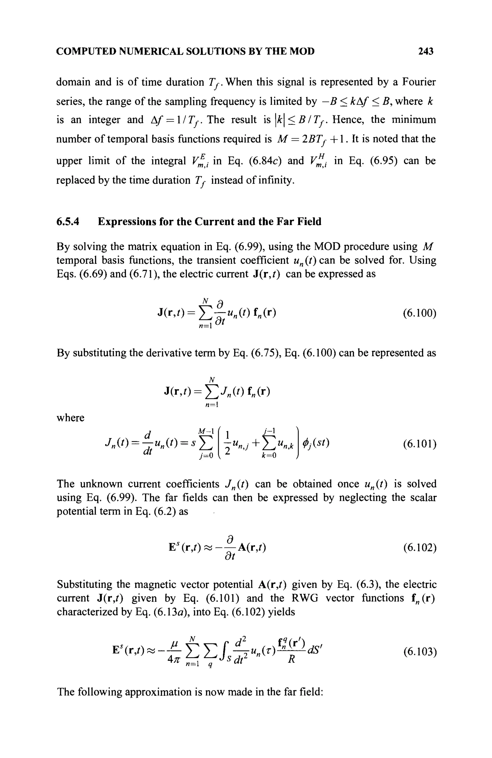
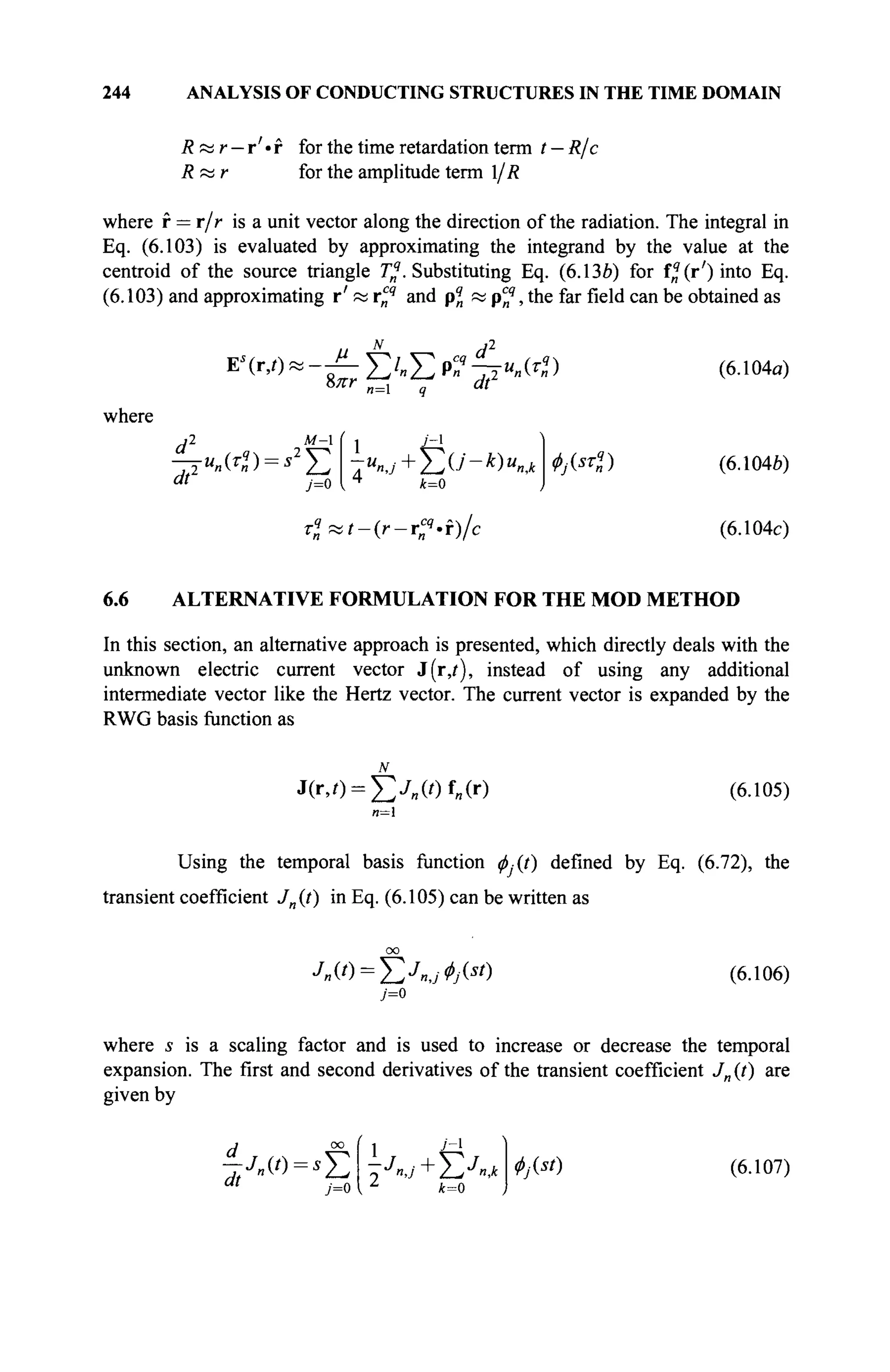
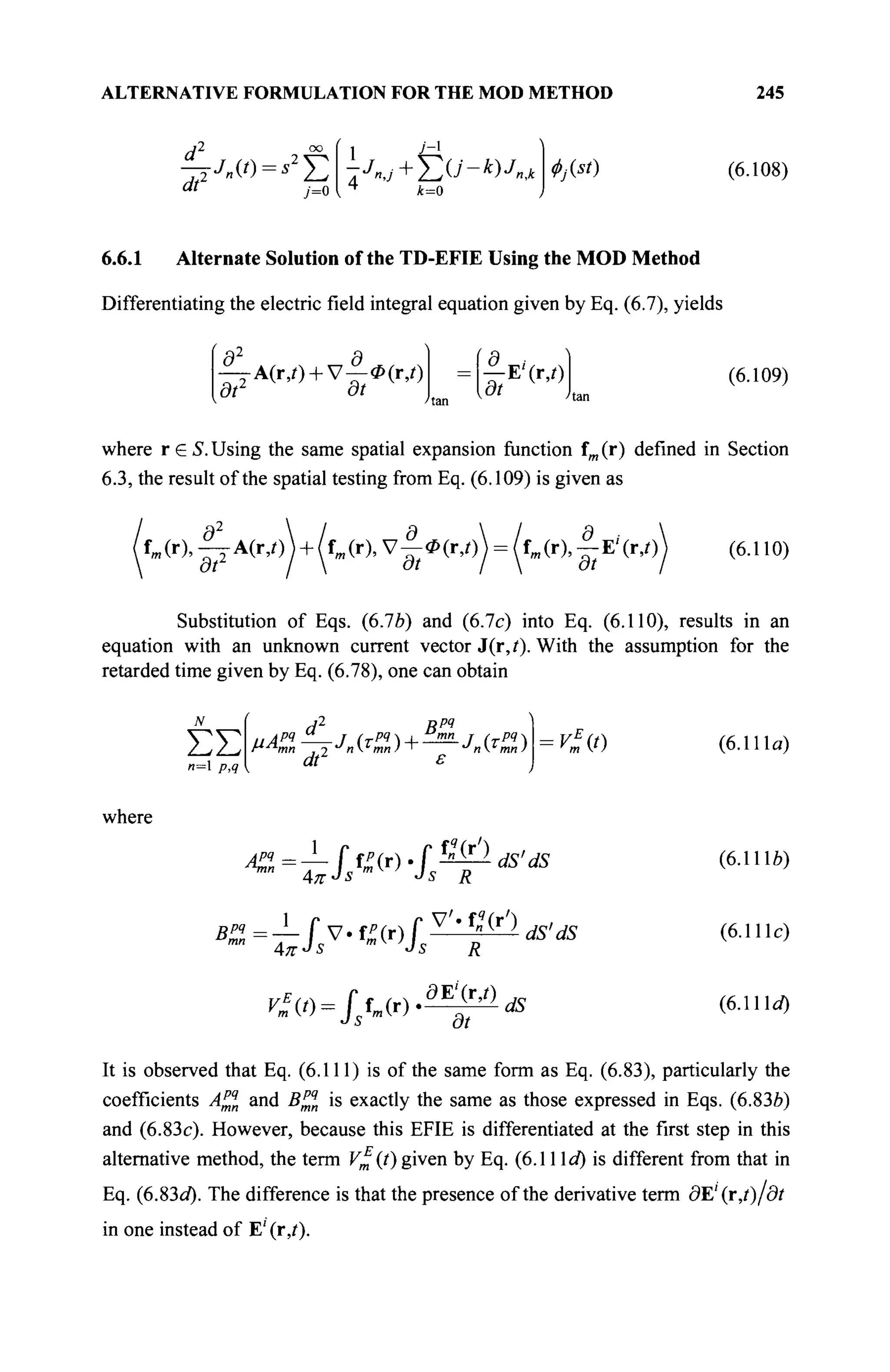
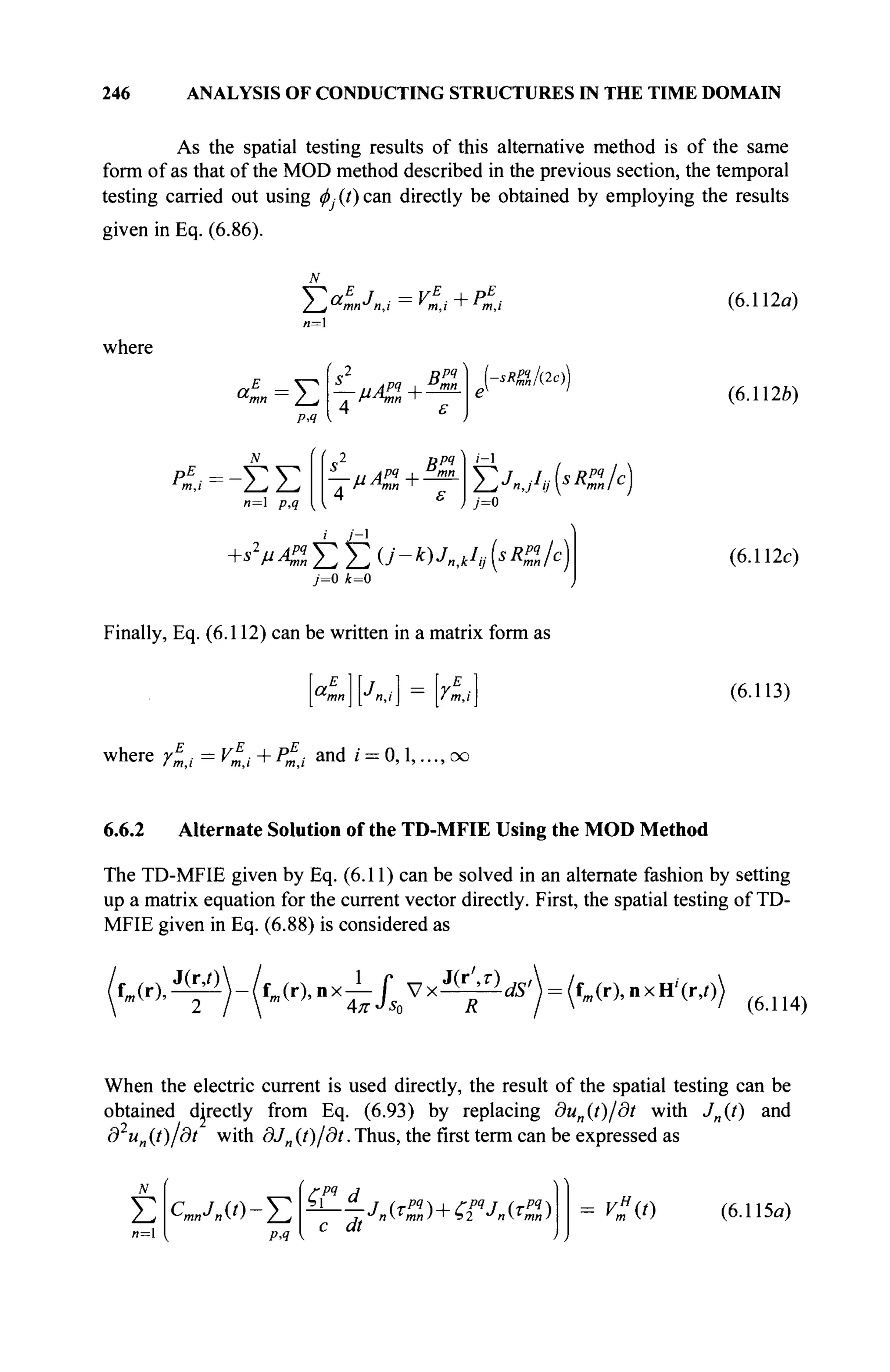
![248 ANALYSIS OF CONDUCTING STRUCTURES IN THE TIME DOMAIN
+s
rpq J_ Jzl
ΣΣ^,ΛΚ-Α)
c
j=o k=0
(6.118c)
Furthermore, Eq. (6.118) can be written into a matrix form as
Κ „ ] [ Λ ν ] = r",t (6.119)
where r"i = V"i + P"i and i = 0,1,..., oo
6.6.3 Alternate Solution of the TD-CFIE Using the MOD Method
The matrix equation of the alternative TD-CFIE is obtained by combining Eqs.
(6.113) and (6.119), which results in
where
К«][Л,,-] = [гт,/] (6.120a)
a
mn = Ka
L + VQ - K
)a
mn (6
· ! 2 0 Й
)
Ym,i = 4l,i + 7(1 - ic)r"j (6.120c)
where the expressions of amn and /m · are of the same form as Eqs. (6.99b) and
(6.99c).
6.6.4 Expressions for the Current and the Far Field
By solving Eq. (6.120) by a MOD algorithm with M temporal basis
functions, the transient current coefficient J„(t) can be obtained approximately
fromEq. (6.106) as
M-l
Jn(t
)=J2J
«J0j(st
y (6.121)
The far field expression is obtained using a similar procedure described in Section
6.5. Neglect the scalar potential term in Eq. (6.2) and obtain the far field as
E s
( r , 0 « - — A(r,0 (6.122)
at](https://image.slidesharecdn.com/timeandfrequencydomainsolutionsofemproblemsusingintegralequationsandahybridmethodologyb-250205130750-568a5ba2/75/Time-and-Frequency-Domain-Solutions-of-EM-Problems-Using-Integral-Equations-and-a-Hybrid-Methodology-B-H-Jung-pdf-269-2048.jpg)
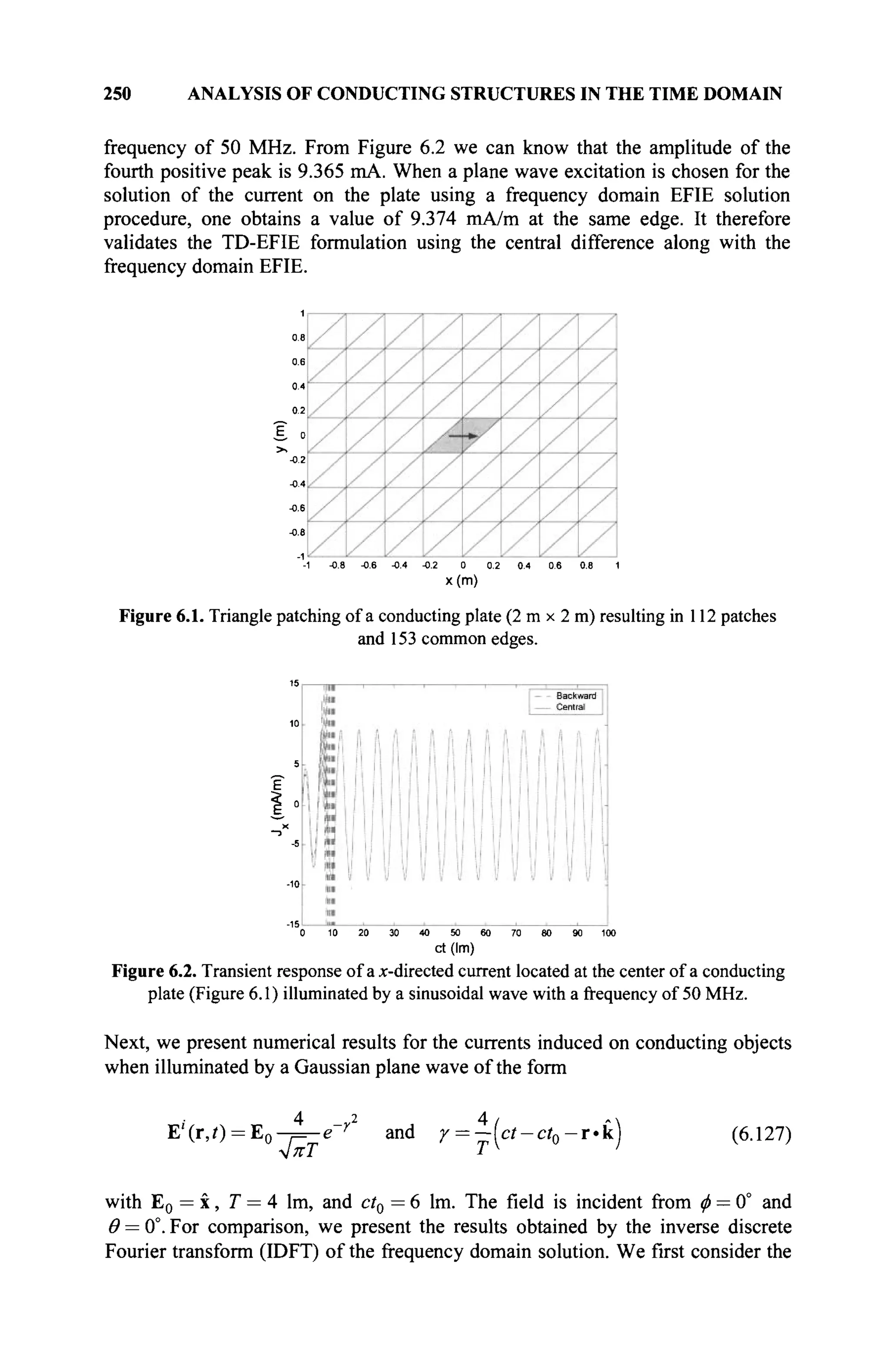
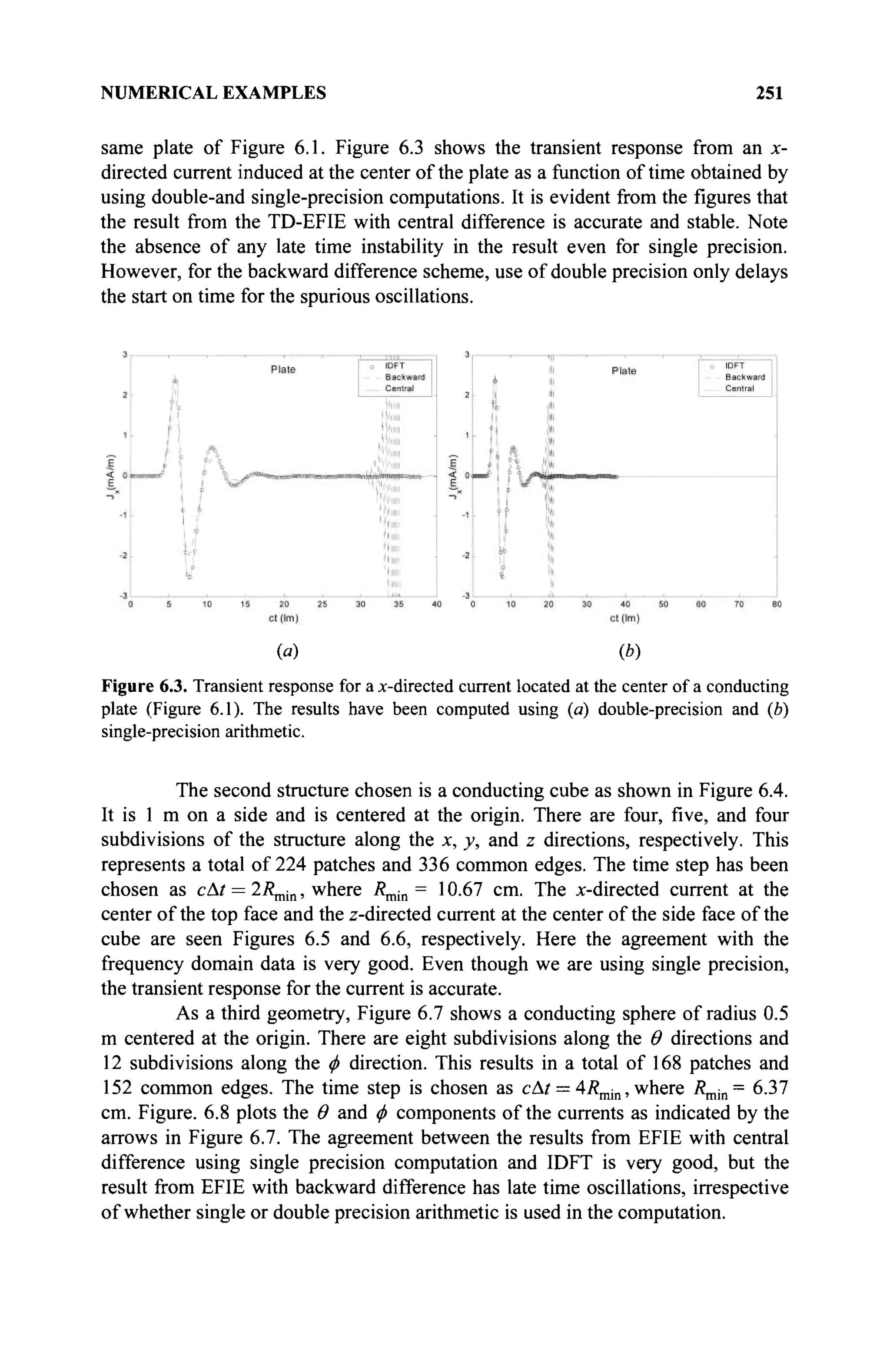
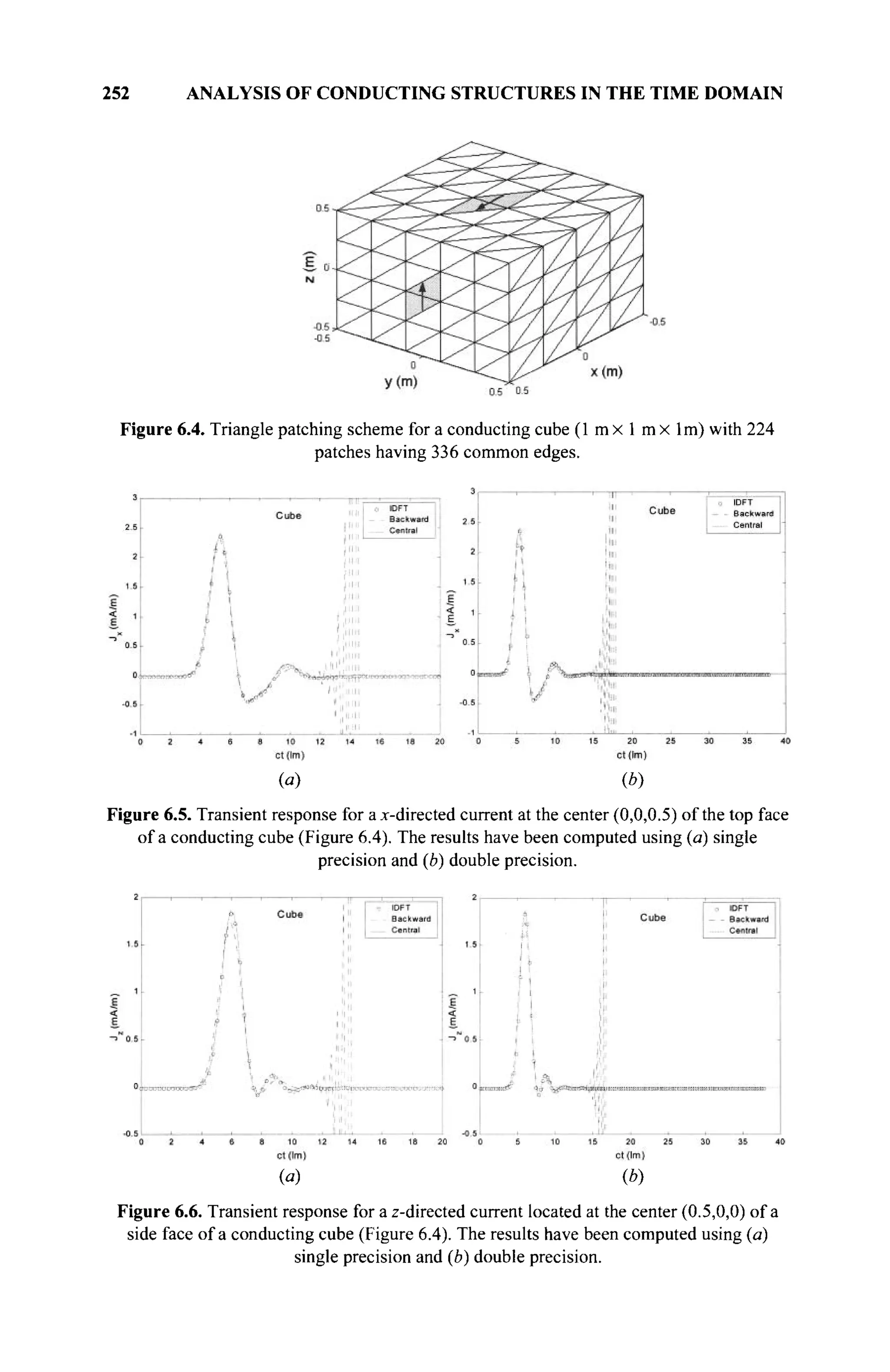
![NUMERICAL EXAMPLES 253
Figure 6.7. Triangle patching of a conducting sphere with a radius 0.5 m resulting in If
patches and 252 common edges.
(«) Ф)
Figure 6.8. Transient response of the current on a conducting sphere (Figure 6.7). (ά) Θ-
component of current at Θ = 90°, φ = 15°. (b) ^-component of current at Θ = 78.75°,
φ = 90°.
6.7.2 Scattering Analysis by Solving the TD-MFIE Using the MOT Method
In this section, we present the numerical results for three-dimensional closed
scatterers, viz. a cube, a sphere, and a cylinder. The scatterers are illuminated by a
Gaussian plane wave in which the magnetic field is given by
1 „ 4 2 4 / «
H'(r,/) = - k x E 0 - = - e r
and y = —ct-ct0 - f k ] (6.128)
with E0 = x, T = A lm, and ct0 = 6 lm. к is the unit propagation vector. The
field is incident from ф = 0° and Θ — 0°. For comparison, we present the results
obtained by TD-EFIE and the IDFT of the frequency domain solution calculated in
the 0-500 MHz interval using 128 samples. There are several methods to deal with
a magnetic vector potential term in the EFIE formulation [1—4]. We use EFIE with](https://image.slidesharecdn.com/timeandfrequencydomainsolutionsofemproblemsusingintegralequationsandahybridmethodologyb-250205130750-568a5ba2/75/Time-and-Frequency-Domain-Solutions-of-EM-Problems-Using-Integral-Equations-and-a-Hybrid-Methodology-B-H-Jung-pdf-274-2048.jpg)
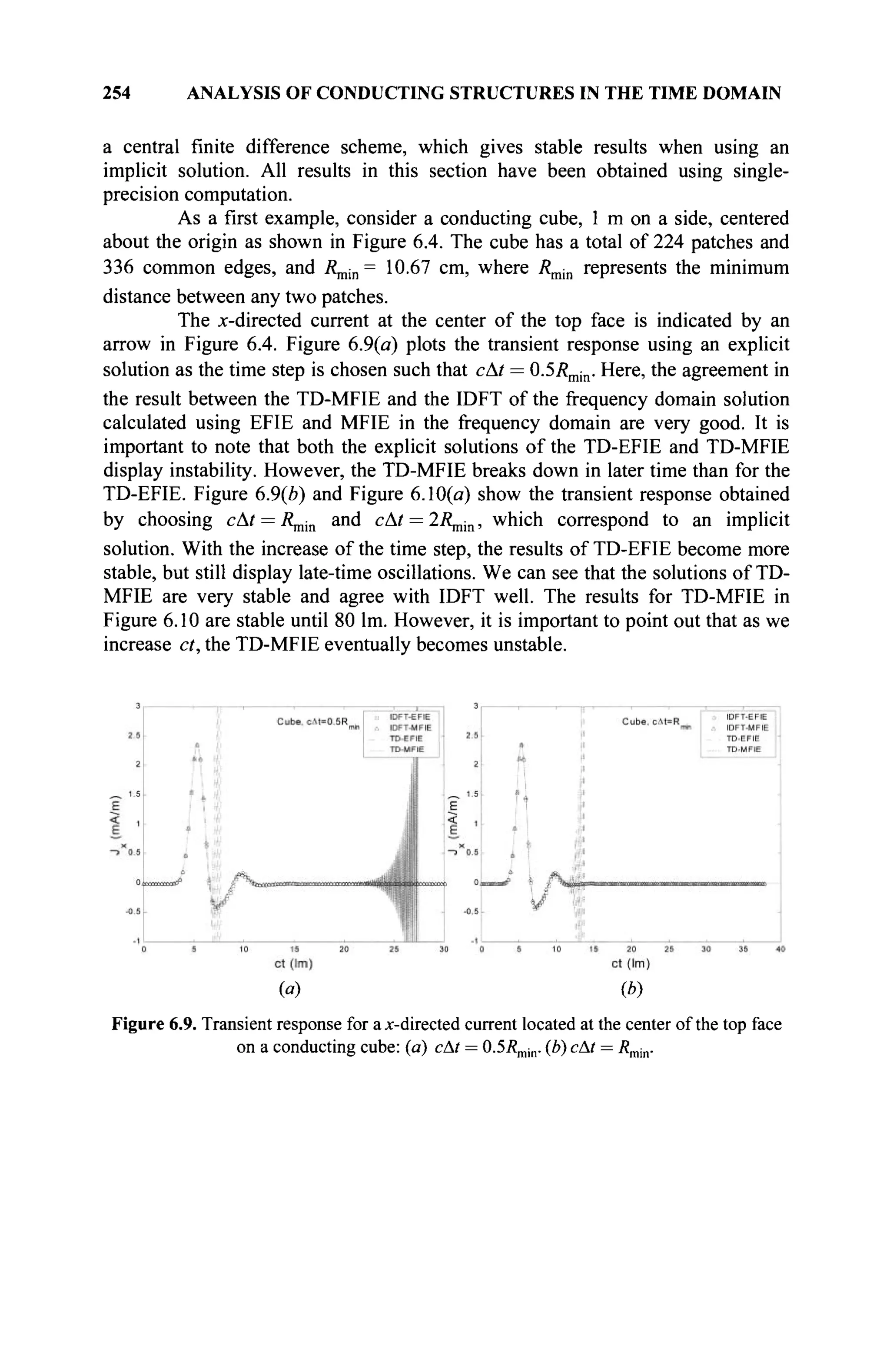
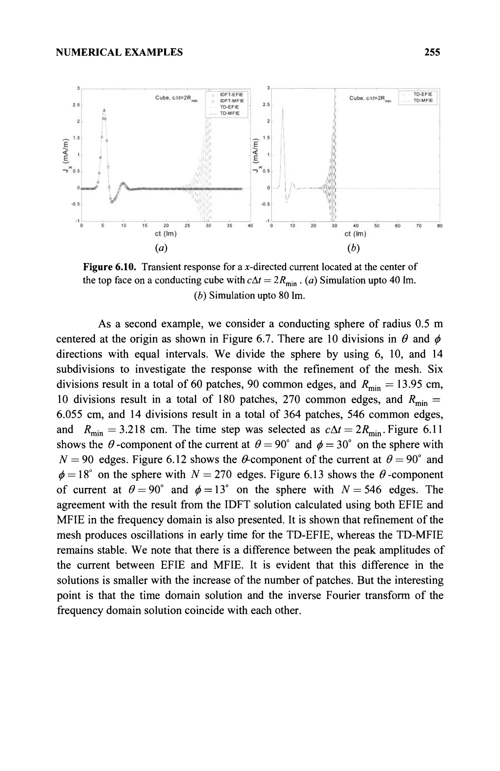
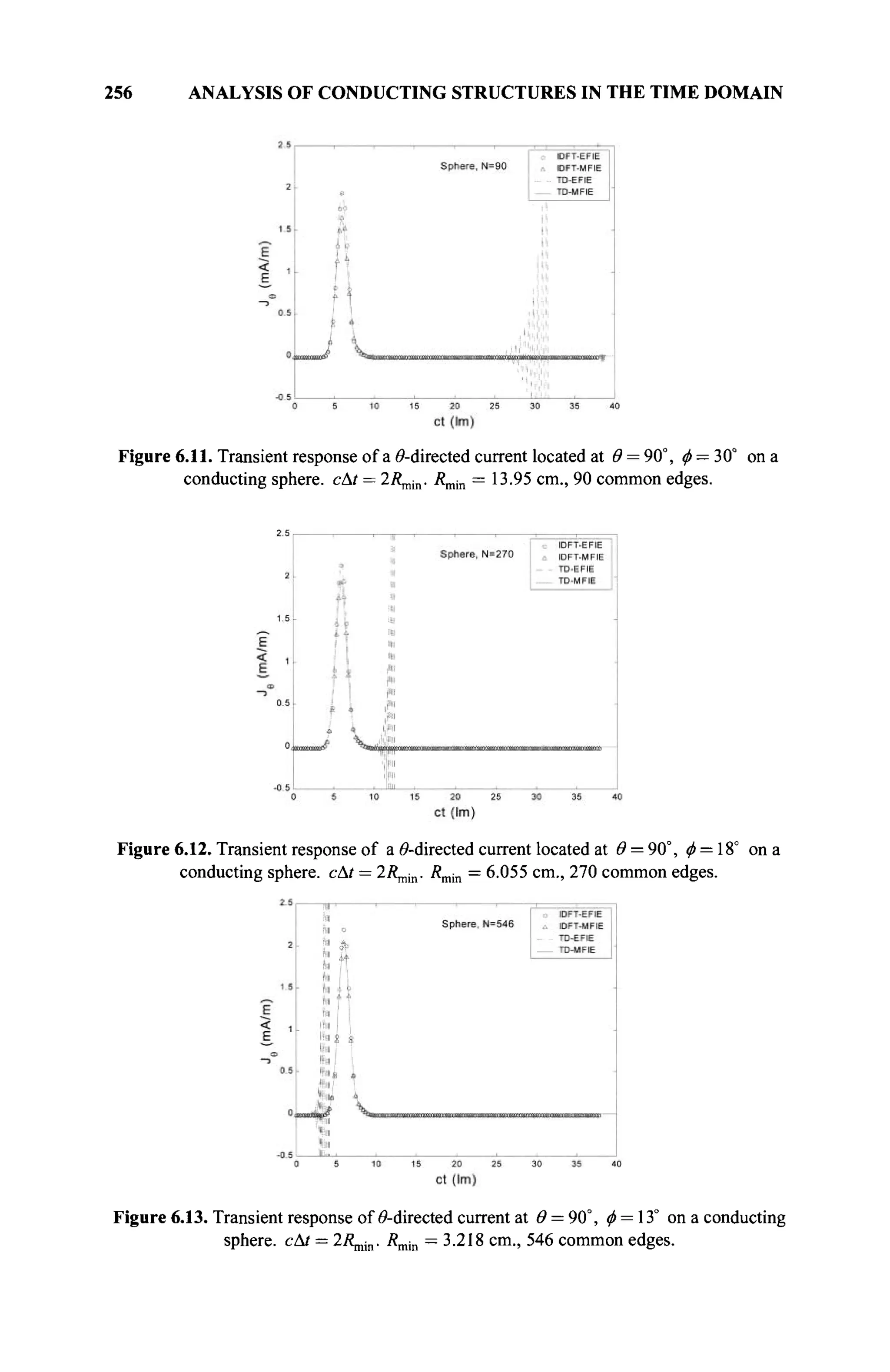
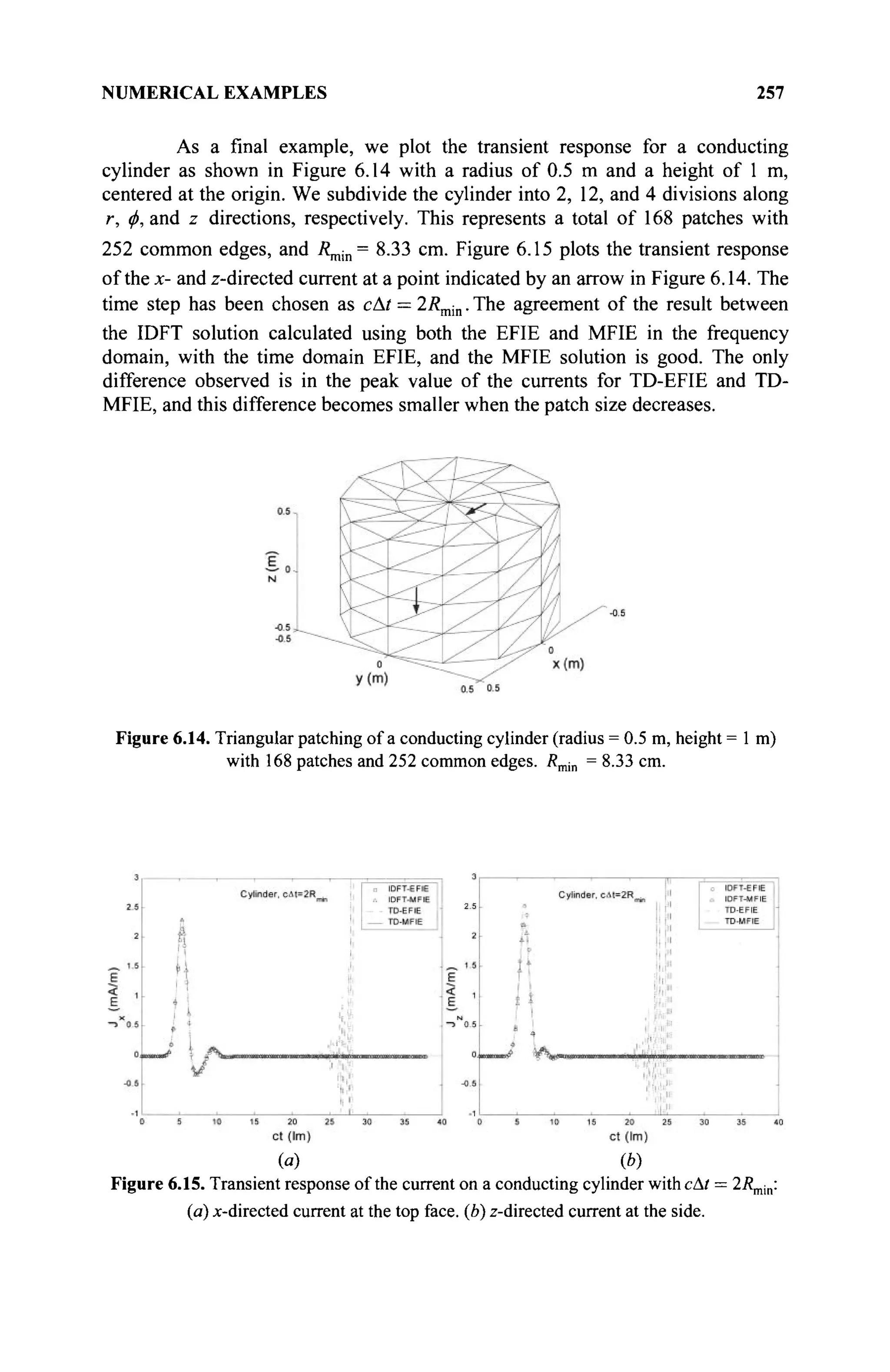
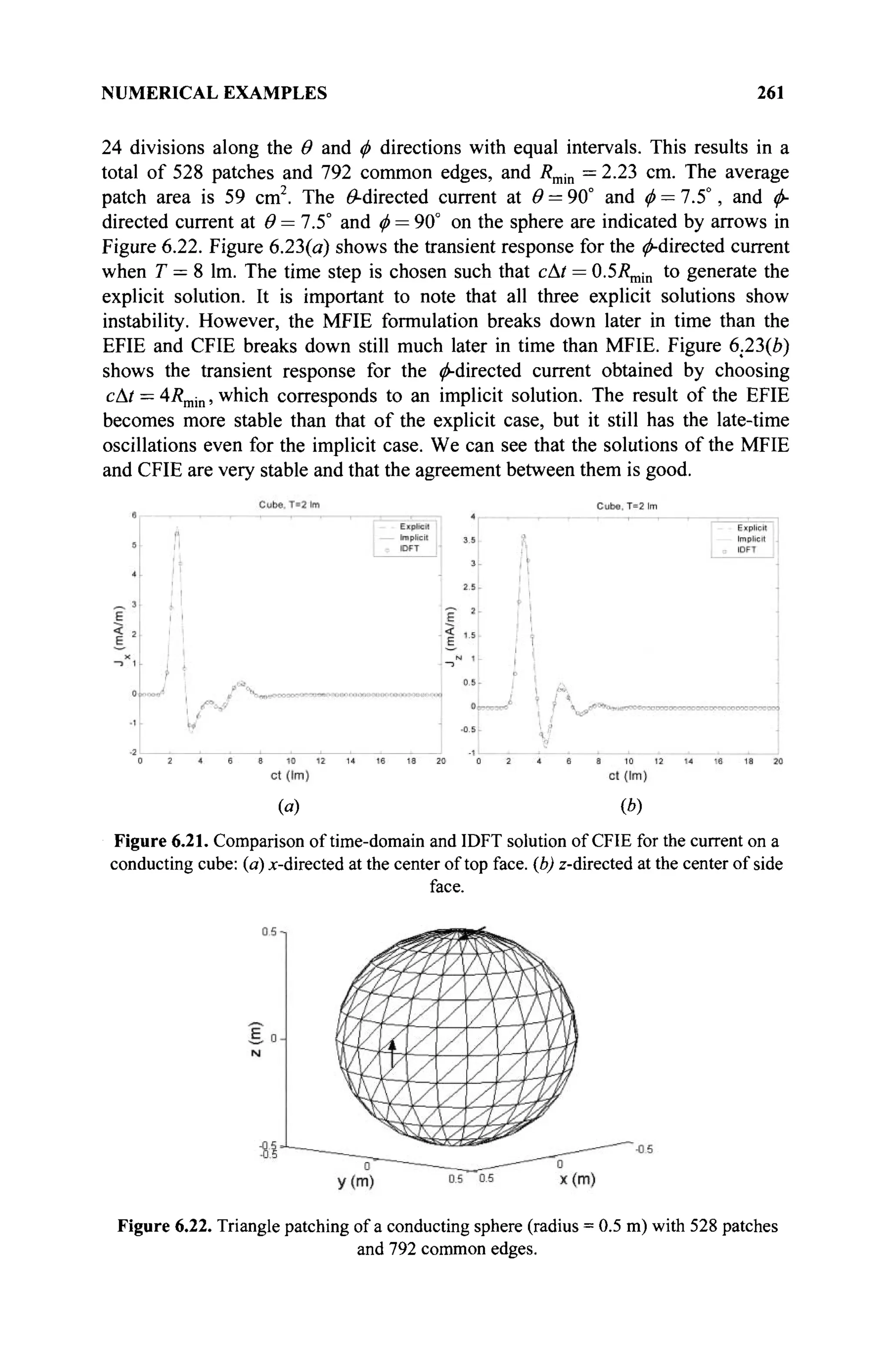
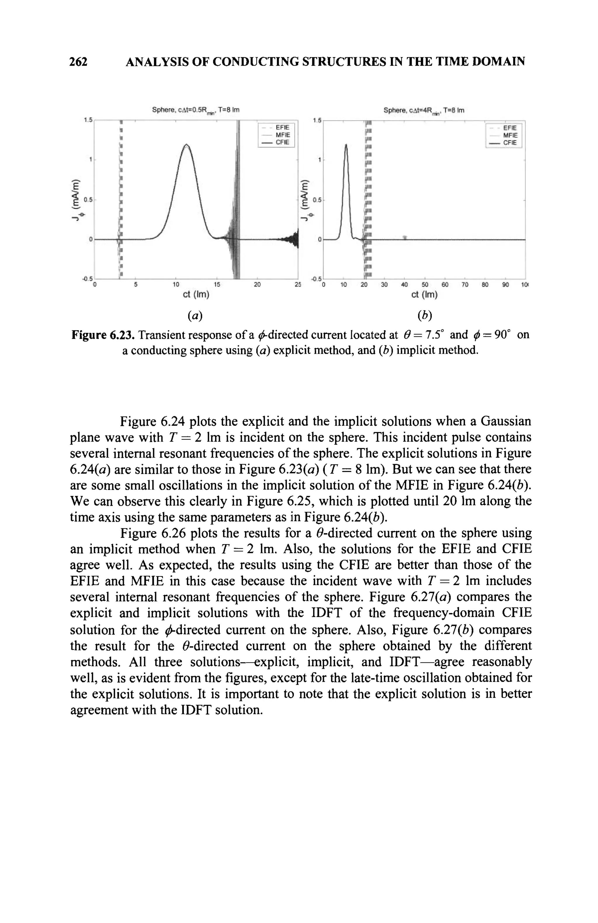
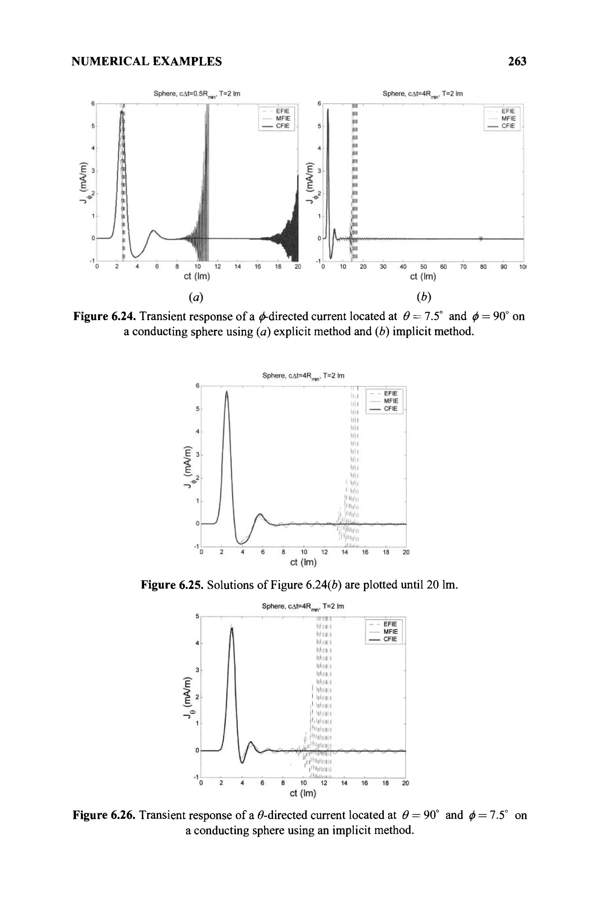
![264 ANALYSIS OF CONDUCTING STRUCTURES IN THE TIME DOMAIN
(a) (b)
Figure 6.27. Comparison of time-domain and IDFT solution of CFIE for the current on a
conducting sphere (a) ^-directed, at Θ = 7.5° and φ = 90°. (b) 0-directed, at θ = 90°, and
ftf = 7.5°
6.7.4 Scattering Analysis by Solving the TDIEs Using the MOD Method
In this section, numerical results from three representative 3-D closed conducting
scatterers, viz. a sphere, a cube, and a cylinder, are presented. The scatterers are
illuminated by a Gaussian plane wave in which the electric and magnetic fields are
given by Eqs. (6.127) and (6.128). The incident field is arriving from φ = 0° and
θ = 0° and E0 = x. First, in the numerical computation, we use a Gaussian pulse
of T = 8 lm and ctQ = 12 lm. This pulse has a frequency spectrum of 125 MHz, so
the internal resonance effects are excluded for the structures. Next, a Gaussian
pulse with T = 2 lm and ct0 = 3 lm is used. This pulse has a frequency spectrum
of 500 MHz, which encompasses several internal resonant frequencies of the
structures. The numerical results to be plotted are the transient currents on the
surface and Θ- (or x-) components of the normalized far fields computed by EFIE,
MFIE, and CFIE formulations. These far scattered fields from the structures are
obtained along the backward direction and, hence, represent the back-scattered
fields. We also present the monostatic radar cross section (RCS) by considering
both Θ- and (^components of the far fields. All numerical solutions have been
computed using the methods presented and are compared with IDFT of the
solutions obtained in the frequency-domain as well as the transient currents using
the MOT method [18]. In addition, the far field solutions for the sphere are
compared with the Mie series solutions. We set s = 109
and M = 80, which is
sufficient to get accurate solutions. In all legends of the figures to be shown, the
numbers 'Г and '2' denote results computed using the MOD formulation of
Section 6.5 and the alternative MOD formulation of section 6.6, respectively.](https://image.slidesharecdn.com/timeandfrequencydomainsolutionsofemproblemsusingintegralequationsandahybridmethodologyb-250205130750-568a5ba2/75/Time-and-Frequency-Domain-Solutions-of-EM-Problems-Using-Integral-Equations-and-a-Hybrid-Methodology-B-H-Jung-pdf-285-2048.jpg)
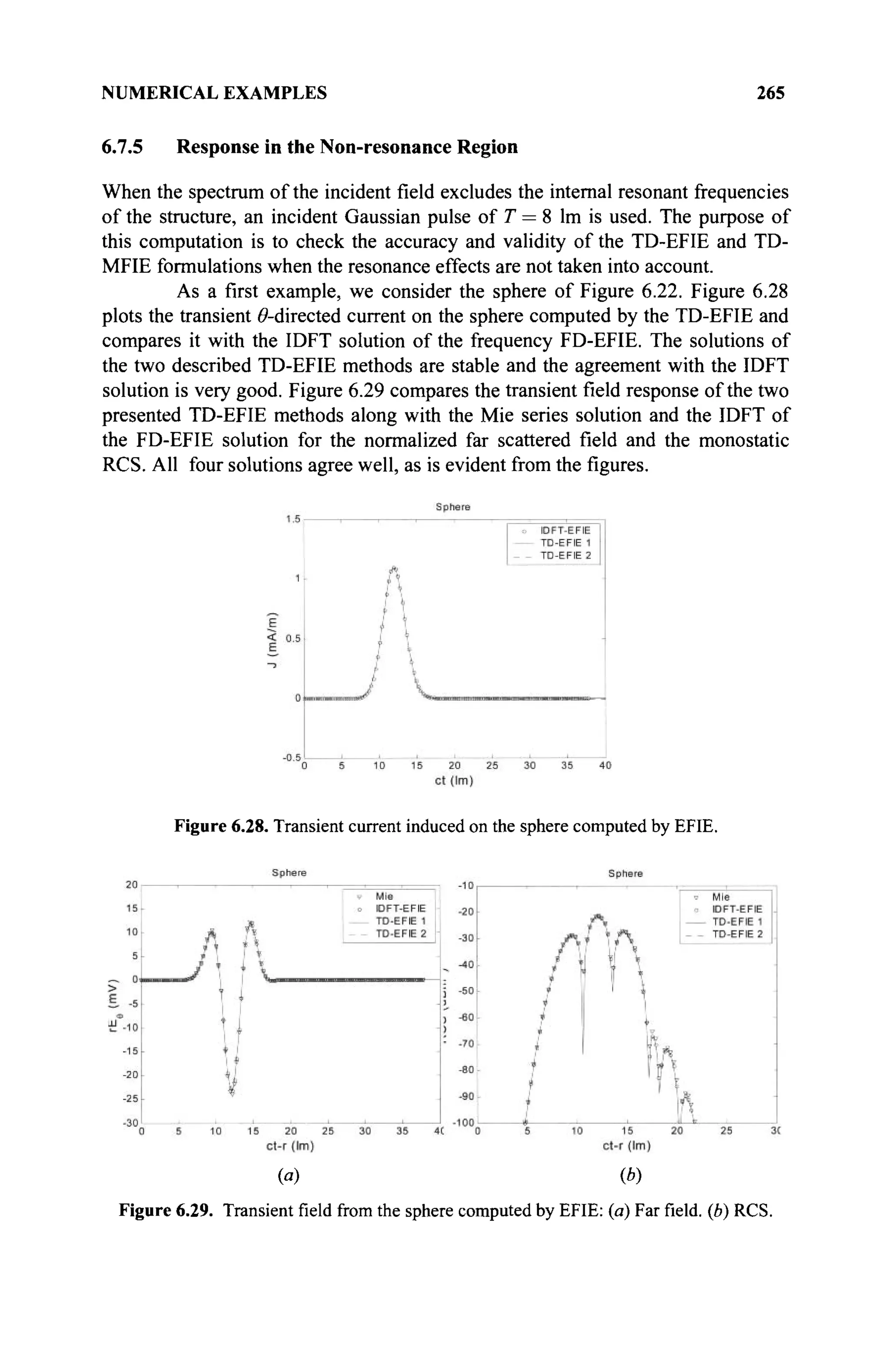
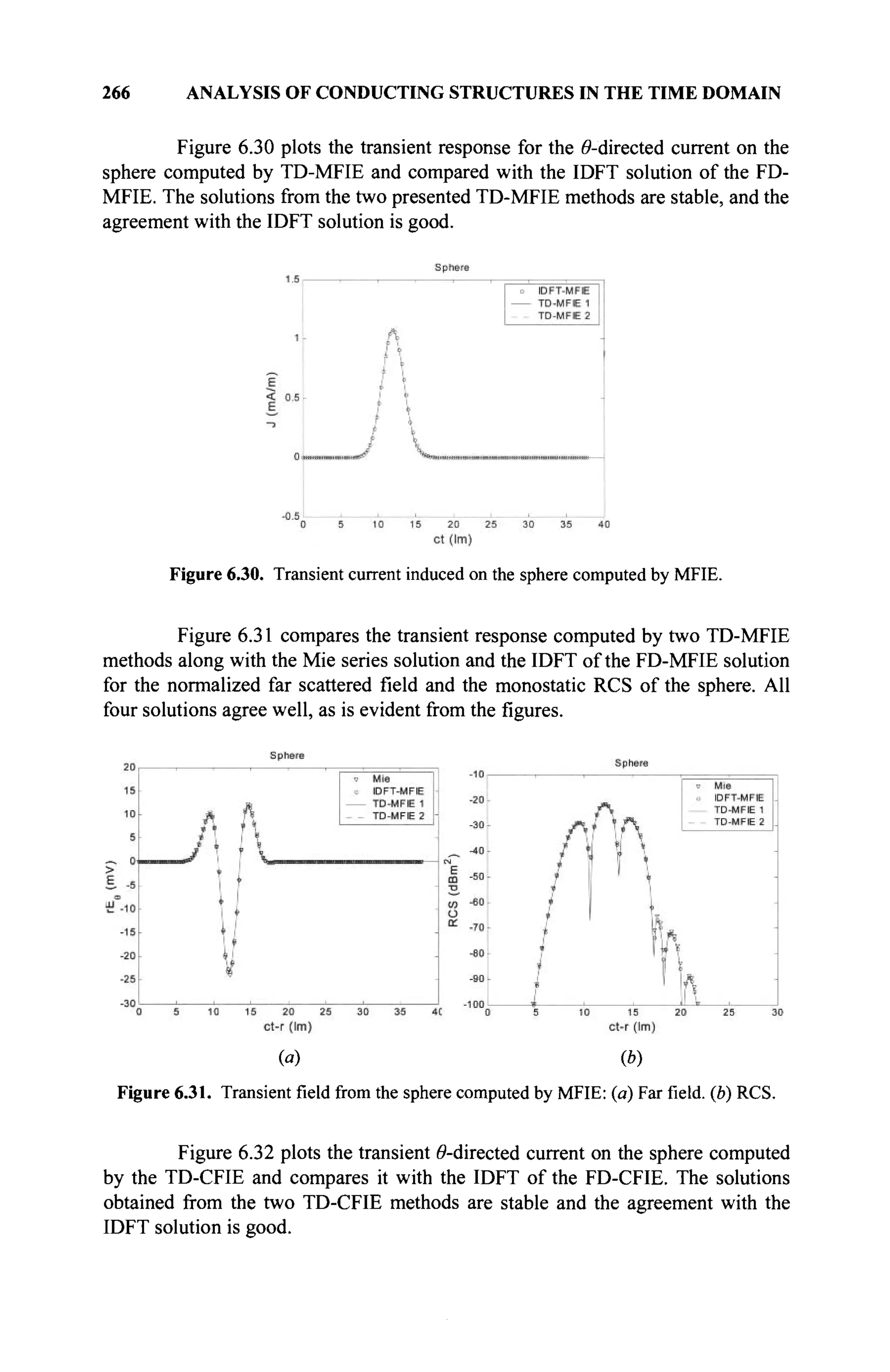
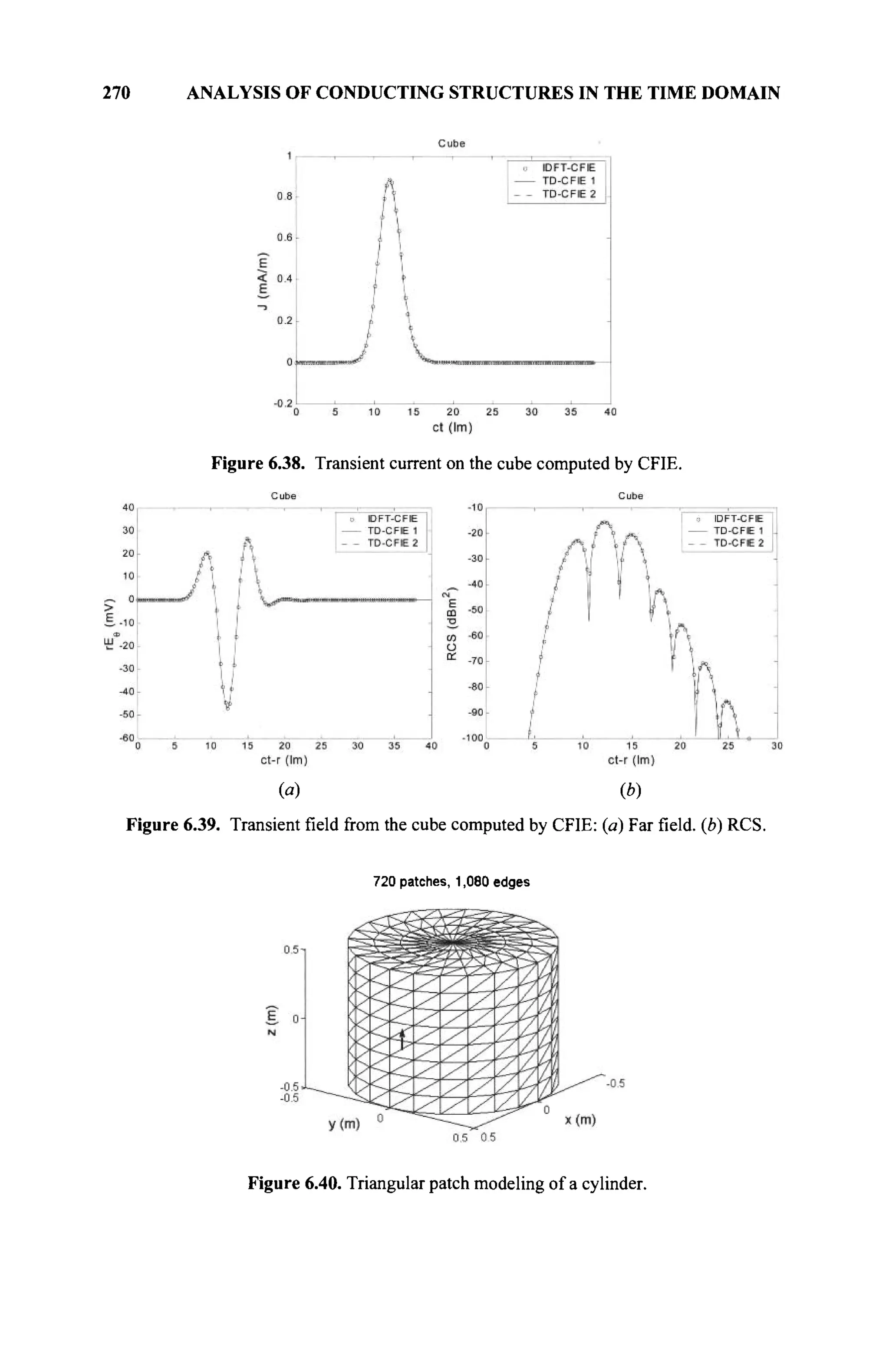
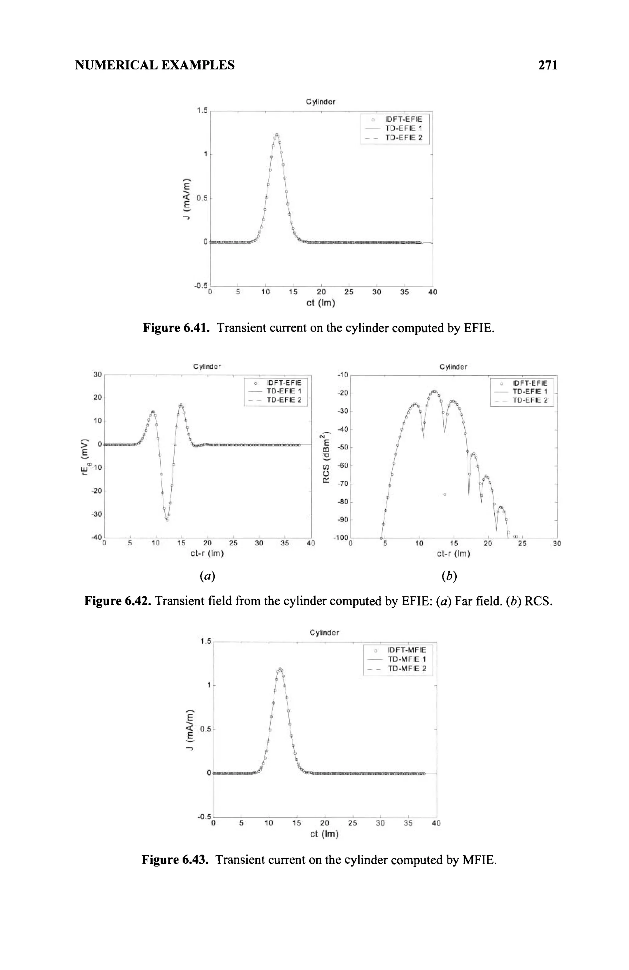
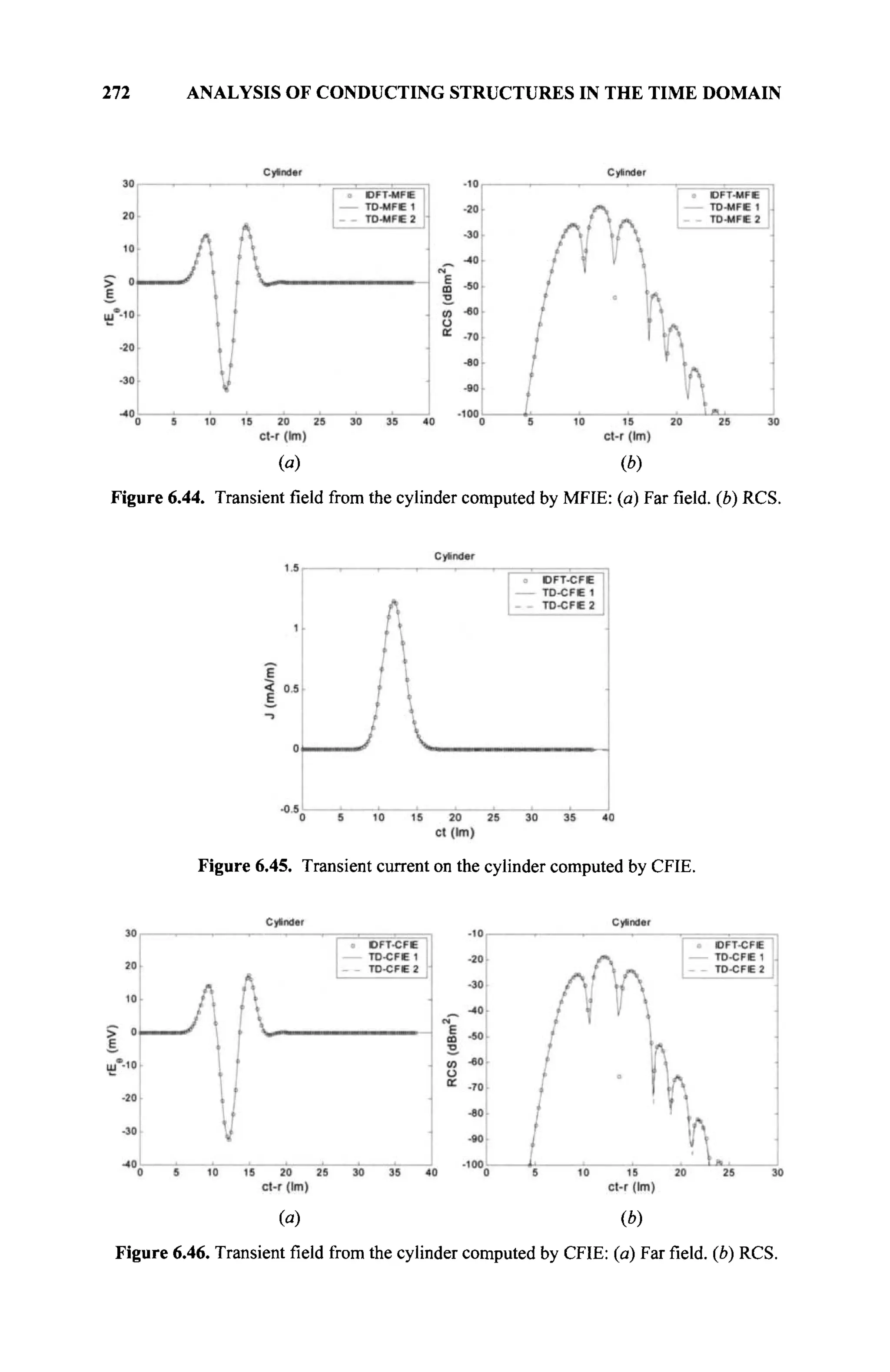
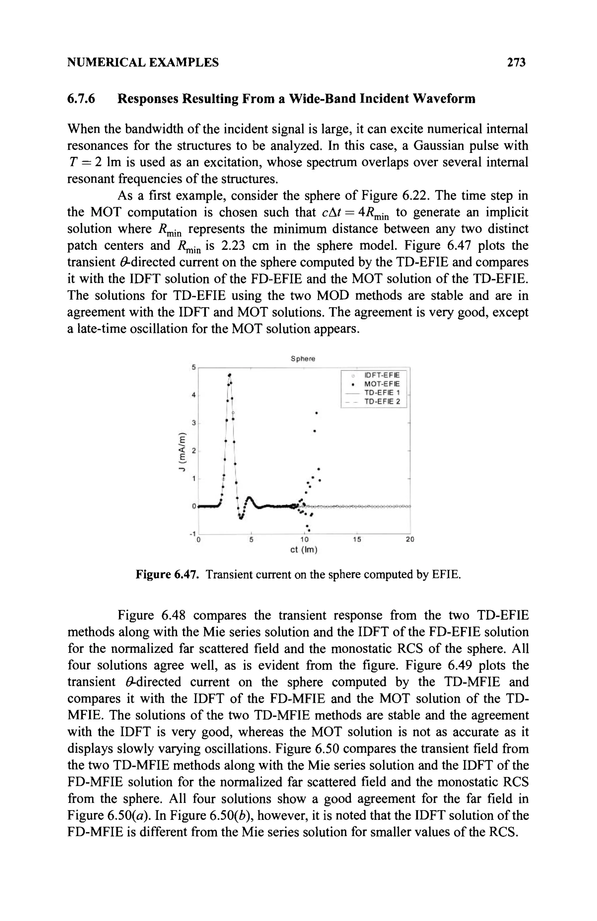
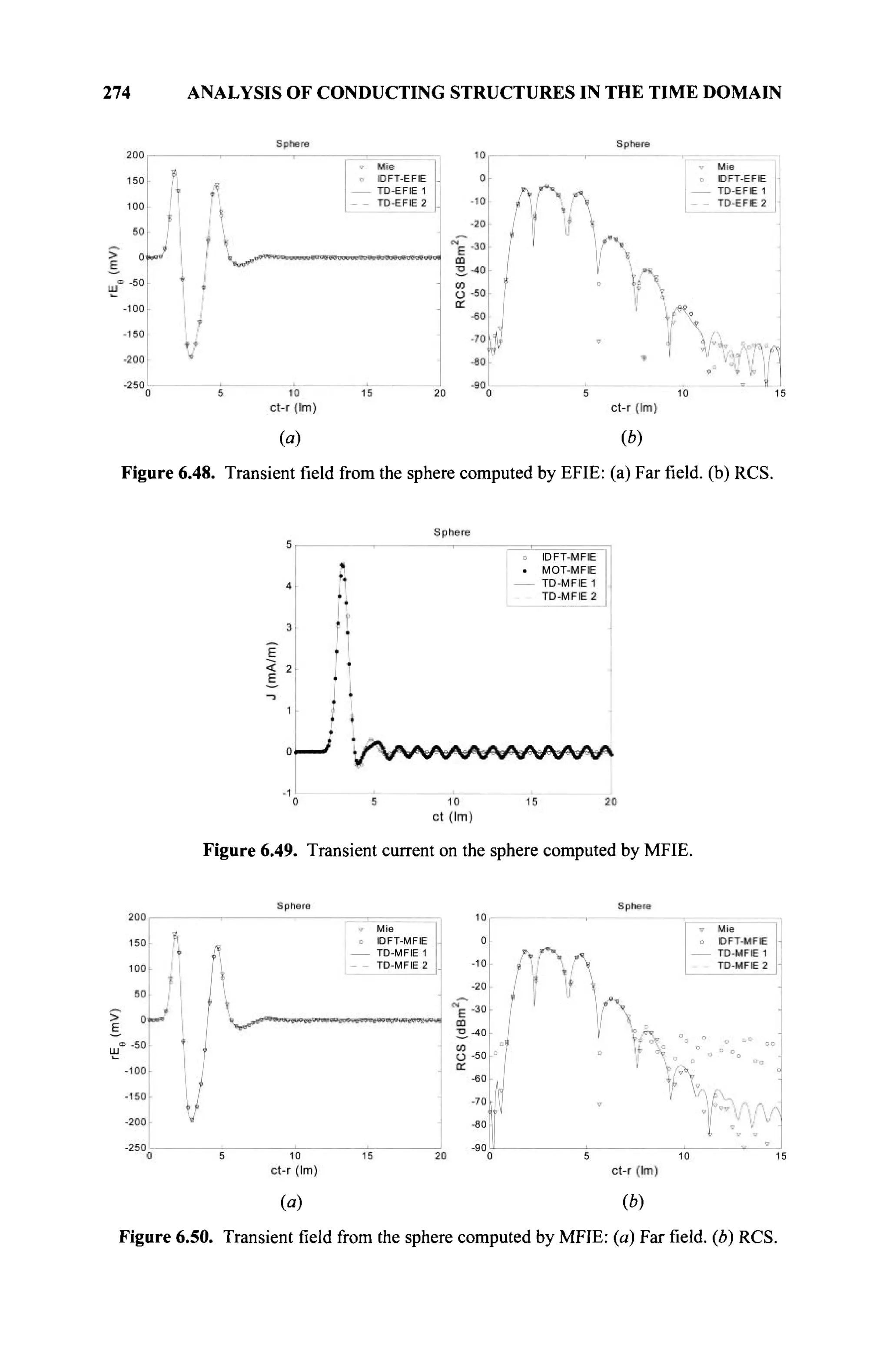
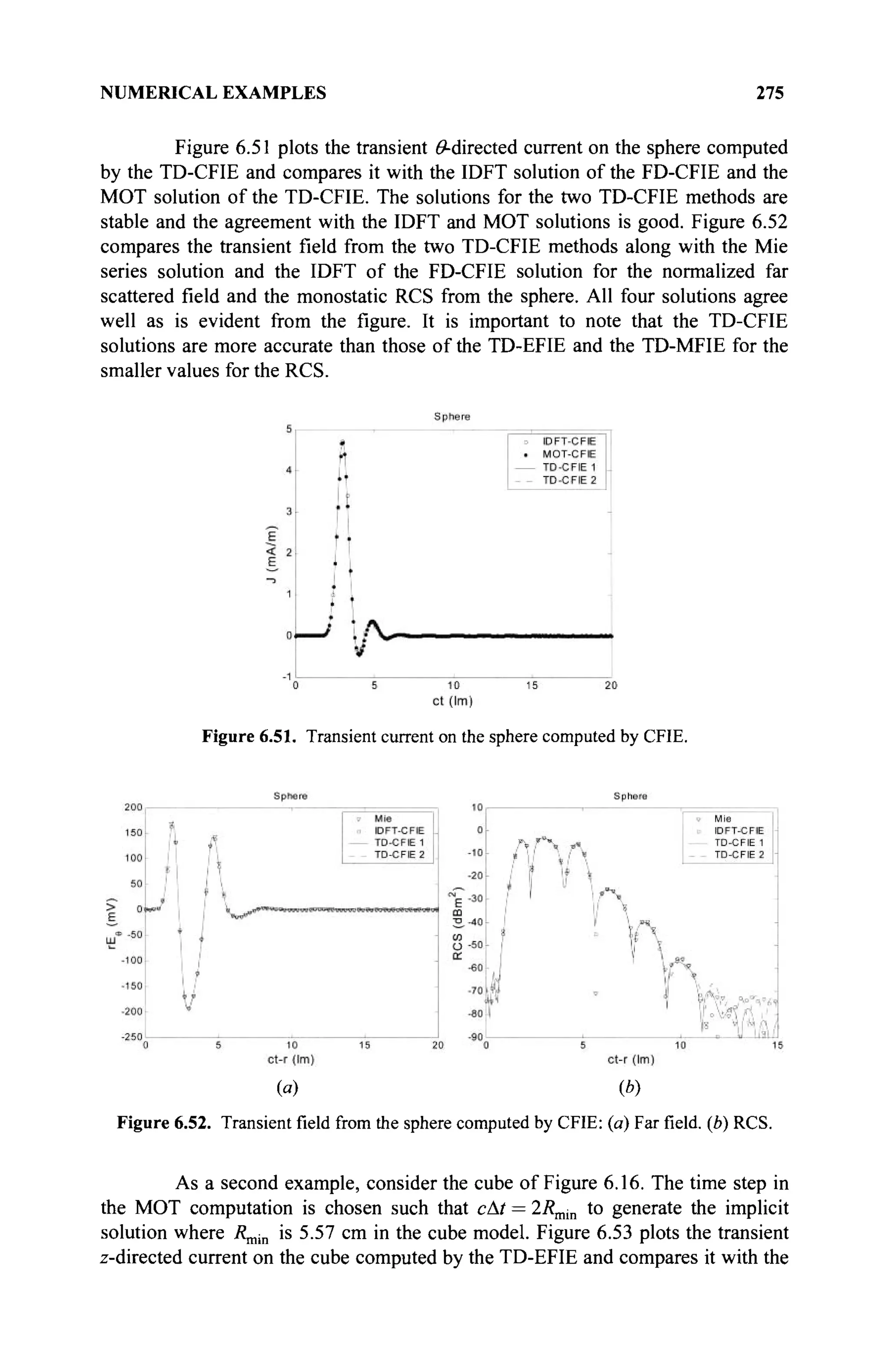
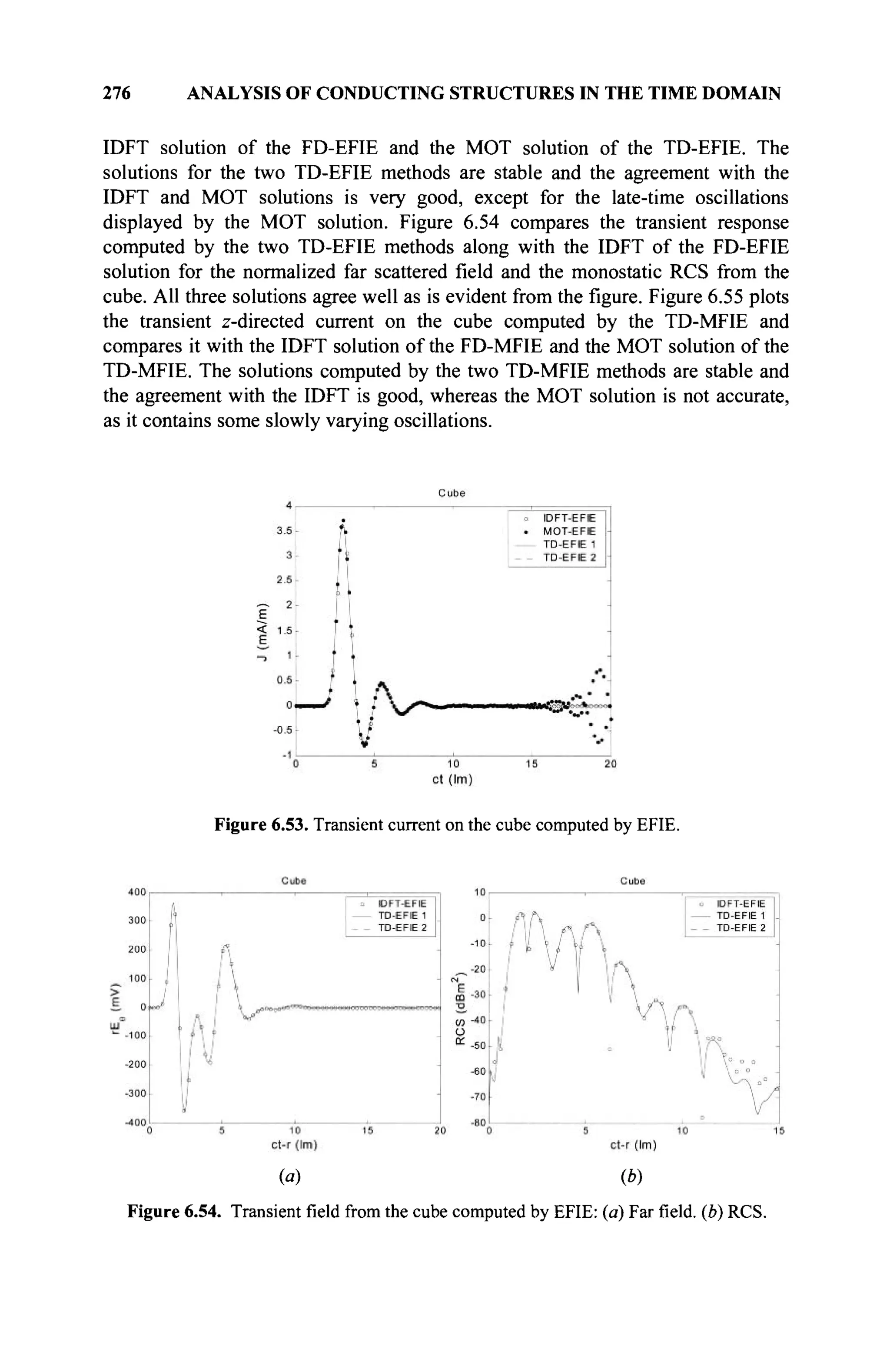
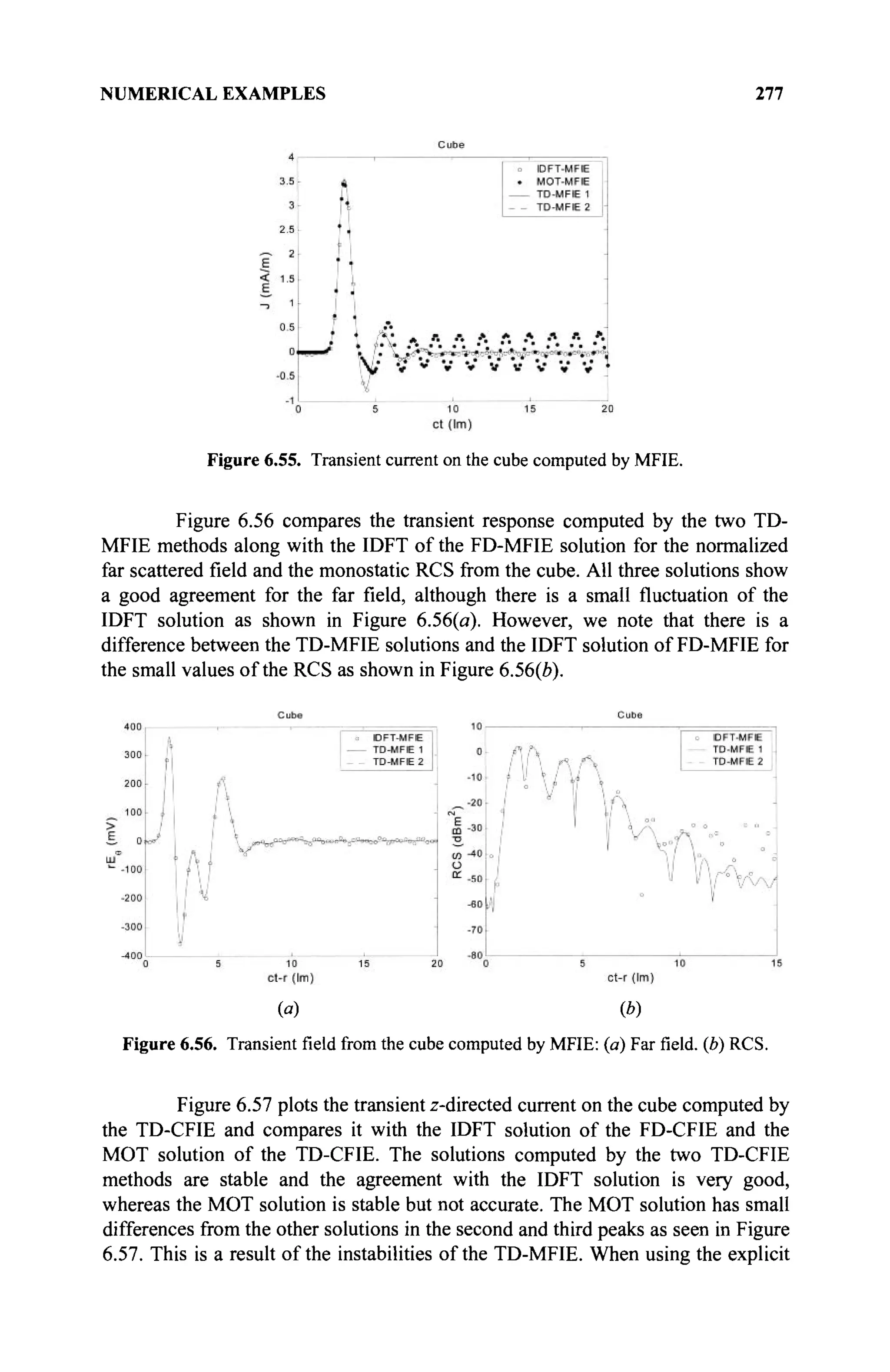
![278 ANALYSIS OF CONDUCTING STRUCTURES IN THE TIME DOMAIN
MOT scheme along with the TD-CFIE, the solution become more accurate, which
has been pointed out in [2]. Figure 6.58 compares the transient field computed by
the two TD-CFIE methods along with the IDFT of the FD-CFIE solution for the
normalized far scattered field and the monostatic RCS for the cube. All three
solutions show a good agreement for the far field as observed in Figure 6.58(a). It
is important to note that solutions for the TD-CFIE show better agreement with the
IDFT solution than those from the TD-EFIE and TD-MFIE for small values of the
RCS.
Figure 6.57. Transient current on the cube computed by CFIE.
(a) (b)
Figure 6.58. Transientfieldfrom the cube computed by CFIE: (a) Farfield,(b) RCS.
As a third example, consider the cylinder of Figure 6.40. The time step in
the MOT computation is chosen such that cat = 4Rmin to generate the implicit
solution where R^,^ is 2.15 cm for the cylinder model. Figure 6.59 plots the
transient response for the z-directed current on the cylinder computed by the TD-](https://image.slidesharecdn.com/timeandfrequencydomainsolutionsofemproblemsusingintegralequationsandahybridmethodologyb-250205130750-568a5ba2/75/Time-and-Frequency-Domain-Solutions-of-EM-Problems-Using-Integral-Equations-and-a-Hybrid-Methodology-B-H-Jung-pdf-299-2048.jpg)

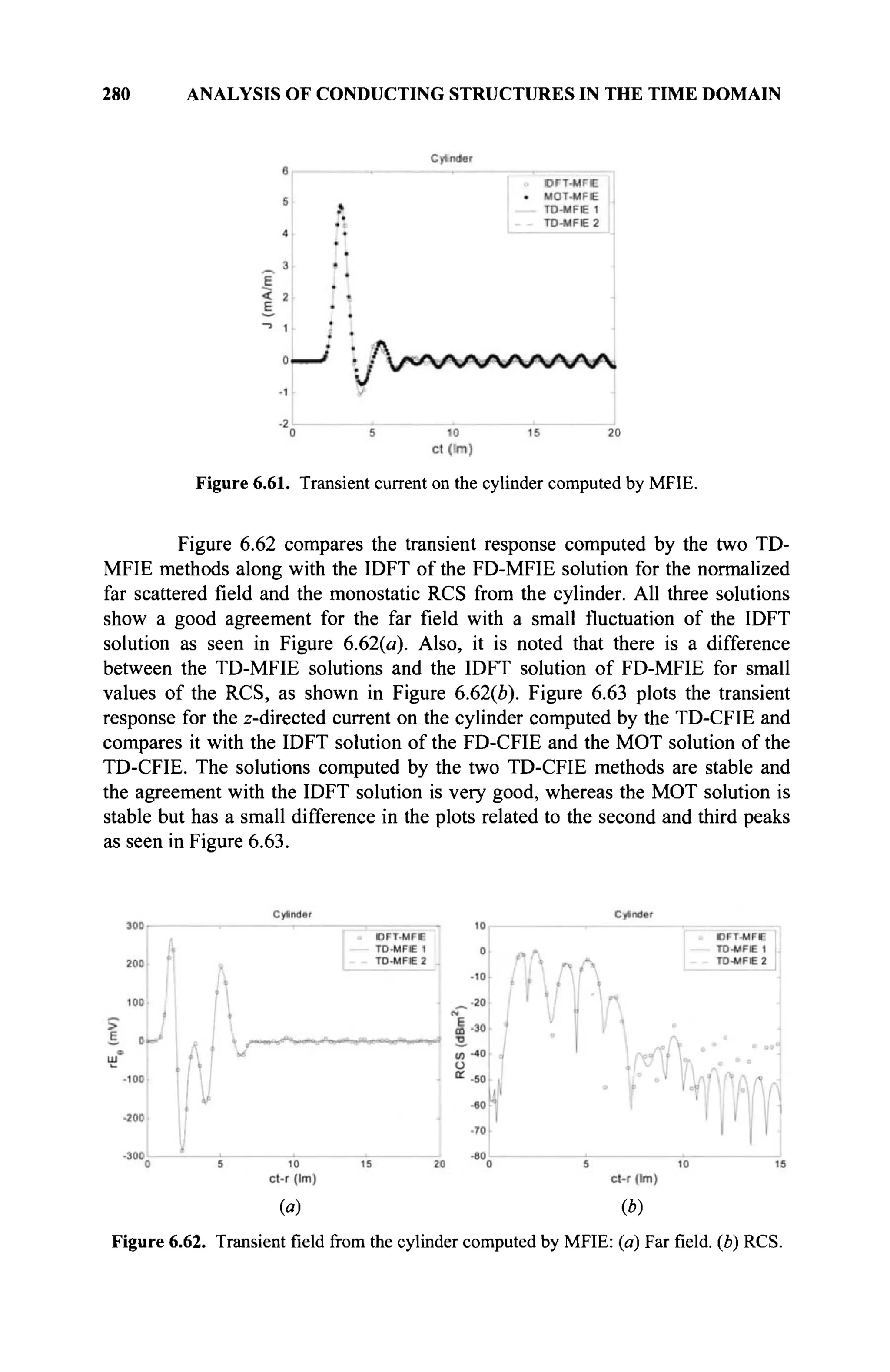
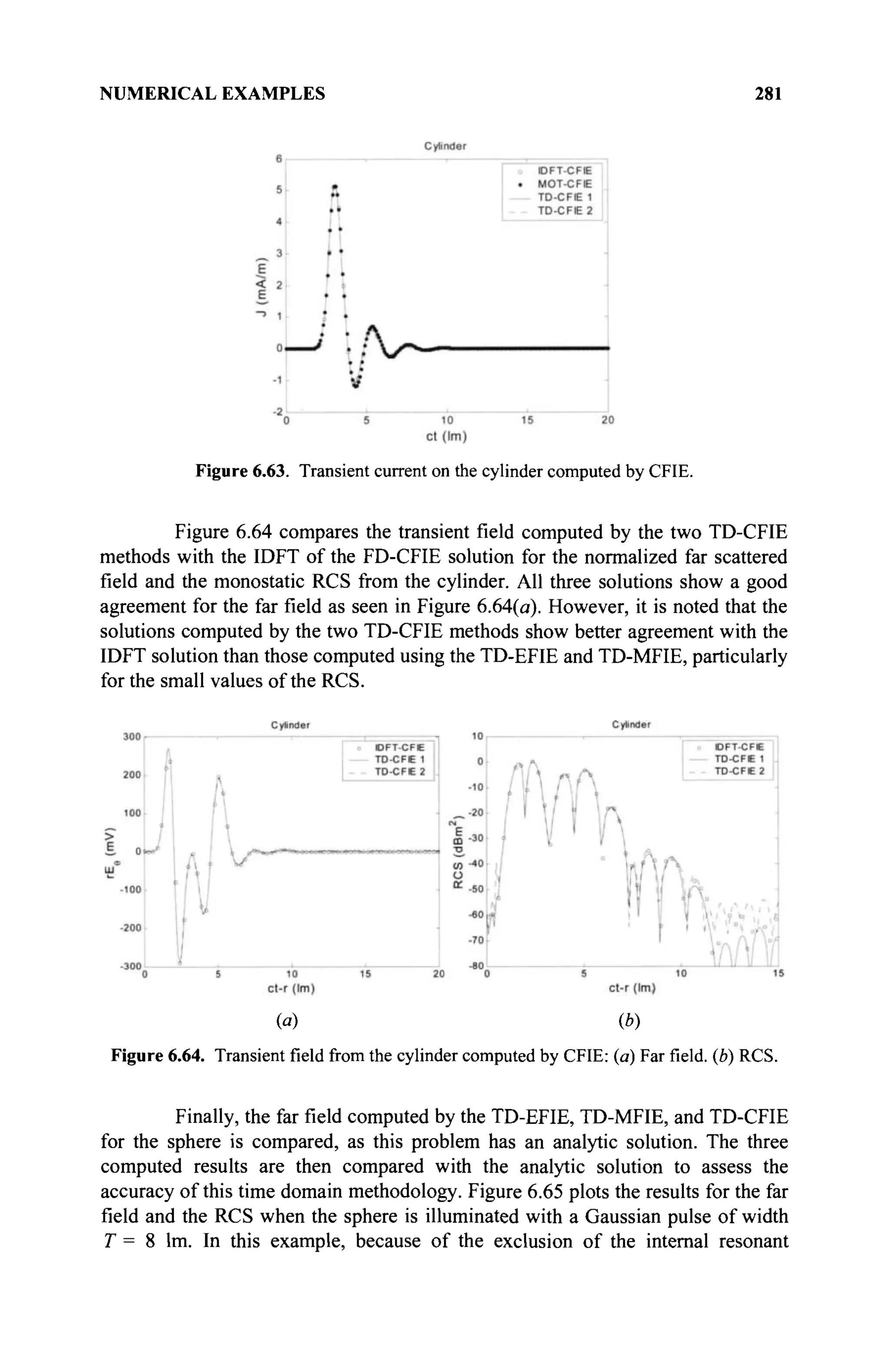
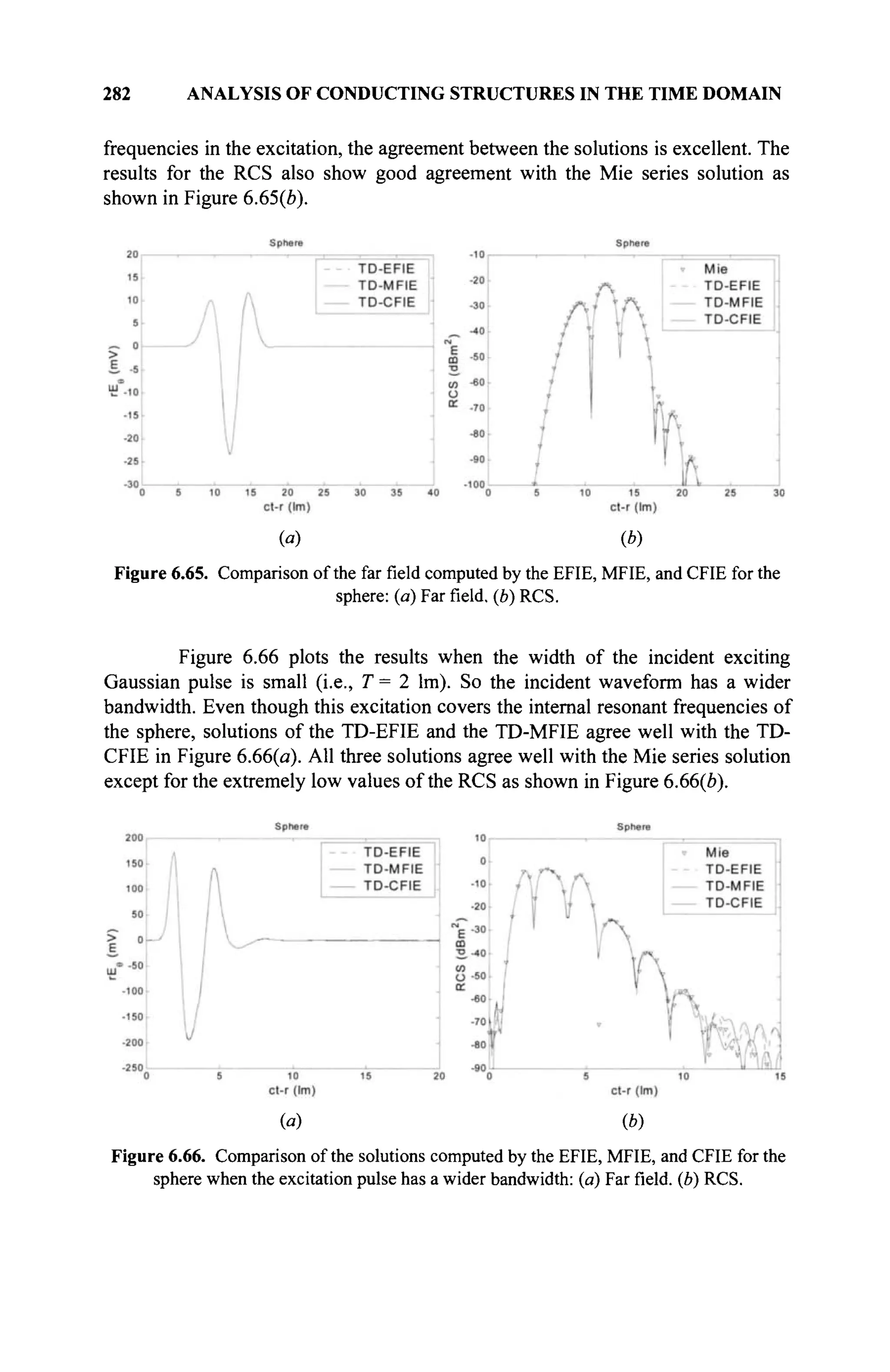
![REFERENCES 283
6.8 CONCLUSION
Two different time domain techniques (the marching-on-in-time and marching-on-
in-degree) have been presented to solve the time domain integral equations for
arbitrarily shaped 3-D conducting structures. In the application of the MoM
procedure, the triangular patch functions have been used as both spatial basis and
testing functions. A temporal basis function set derived from the Laguerre
polynomials has been introduced in the marching-on-in-degree method. The
advantage of this new method is to guarantee the late time stability of the
computed solutions. With the representation of the derivative of the transient
coefficient in an analytic form, the temporal derivatives in the integral equations
can be treated analytically when using the associated Laguerre functions as both
temporal testing and basis functions. In this way, one can do away with the
Courant-Friedrich-Levy criteria relating the spatial discretizations with the
temporal ones. Transient electric current and the far field computed by the two
methods have been accurate and stable. The agreement between the solutions
obtained using the two presented methods with the IDFT of the frequency domain
solution are very good.
REFERENCES
[1] S. M. Rao and D. R. Wilton, "Transient scattering by conducting surfaces of arbitrary
shape,"IEEE Trans. Antennas Prop., Vol. 39, pp. 56-61,1991.
[2] D. A. Vechinski and S. M. Rao, "A stable procedure to calculate the transient
scattering by conducting surfaces of arbitrary shape," IEEE Trans. Antennas Prop.,
Vol. 40, pp. 661-665, 1992.
[3] D. A. Vechinski, Direct Time Domain Analysis of Arbitrarily Shaped Conducting
or Dielectric Structures Using Patch Modeling Techniques. PhD Dissertation,
Auburn, Ala., 1992.
[4] S. M. Rao and T. K. Sarkar, "An alternative version of the time-domain electric field
integral equation for arbitrarily shaped conductors," IEEE Trans. Antennas Prop.,
Vol. 41, pp. 831-834, 1993.
[5] S. M. Rao, Time Domain Electromagnetics. Academic Press, New York, 1999.
[6] A. Sadigh and E. Arvas, "Treating the instabilities in marching-on-in-time method
from a different perspective," IEEE Trans. Antennas Prop., Vol. 41, pp. 1695-1702,
1993.
[7] P. J. Davies, "On the stability of time-marching schemes for the general surface
electric-field integral equation," IEEE Trans. Antennas Prop., Vol. 44, pp. 1467—
1473, 1996.
[8] S. M. Rao and T. K. Sarkar, "An efficient method to evaluate the time-domain
scattering from arbitrarily shaped conducting bodies," Microw. Opt. Tech. Lett,
Vol. 17, pp. 321-325, 1998.
[9] S. M. Rao, D. A. Vechinski, and T. K. Sarkar, "Transient scattering by conducting
cylinders-implicit solution for the transverse electric case," Microw. Opt. Tech.
Lett, Vol. 21, pp. 129-134, 1999.
[10] T. K. Sarkar, W. Lee, and S. M. Rao, "Analysis of transient scattering from
composite arbitrarily shaped complex structures," IEEE Trans. Antennas Prop., Vol.
48, pp. 1625-1634,2000.](https://image.slidesharecdn.com/timeandfrequencydomainsolutionsofemproblemsusingintegralequationsandahybridmethodologyb-250205130750-568a5ba2/75/Time-and-Frequency-Domain-Solutions-of-EM-Problems-Using-Integral-Equations-and-a-Hybrid-Methodology-B-H-Jung-pdf-304-2048.jpg)
![284 ANALYSIS OF CONDUCTING STRUCTURES IN THE TIME DOMAIN
[11] S. M. Rao and T. K. Sarkar, "Time-domain modeling of two-dimensional
conducting cylinders utilizing an implicit scheme-TM incidence," Microw. Opt.
Tech. Lett, Vol. 15, pp. 342-347, 1997.
[12] S. M. Rao and T. K. Sarkar, "Transient analysis of electromagnetic scattering from
wire structures utilizing an implicit time-domain integral-equation technique,"
Microw. Opt. Tech. Lett, Vol. 17, pp. 66-69, 1998.
[13] B. H. Jung and T. K. Sarkar, "Time-domain electric-field integral equation with
central finite difference," Microw. Opt. Tech. Lett., Vol. 31, pp. 429^135, 2001.
[14] B. H. Jung, T. K. Sarkar, Y.-S. Chung, and Z. Ji, "An accurate and stable implicit
solution for transient scattering and radiation from wire structures," Microw. Opt.
Tech. Lett, Vol. 34, pp. 354-359, 2002.
[15] B. H. Jung and T. K. Sarkar, "Transient scattering from three-dimensional
conducting bodies by using magnetic field integral equation," J. Electromagn.
Waves Appl, Vol. 16, pp. 111-128, 2002.
[16] D. A. Vechinski and S. M. Rao, "Transient scattering by dielectric cylinders: e-
field, h-field, and combined field solutions," Radio Sei., Vol. 27, pp. 611-622,
1992.
[17] B. Shankar, A. A. Ergin, K. Aygun, and E. Michielssen, "Analysis of transient
electromagnetic scattering from closed surfaces using a combined field integral
equation," IEEE Trans. Antennas Prop., Vol. 48, pp. 1064-1074,2000.
[18] B. H. Jung and T. K. Sarkar, "Time-domain CFIE for the analysis of transient
scattering from arbitrarily shaped 3D conducting objects," Microw. Opt Tech.
Lett, Vol. 34, pp. 289-296, 2002.
[19] T. K. Sarkar and J. Koh, "Generation of a wide-band electromagnetic response
through a Laguerre expansion using early-time and low-frequency data," IEEE
Trans. Antennas Prop., Vol. 50, pp. 1408-1416, 2002.
[20] S. M. Rao, D. R. Wilton and A. W. Glisson, "Electromagnetic scattering by surfaces
of arbitrary shape," IEEE Trans. Antennas Prop., Vol. 30, pp. 409^*18, 1982.
[21] D. R. Wilton, S. M. Rao, A. W. Glisson, D. H. Schaubert, О. M. Al-Bundak, and
С. M. Butler, "Potential integrals for uniform and linear source distributions on
polygonal and polyhedral domains," IEEE Trans. Antennas Prop., Vol. 32, pp.
276-281, 1984.
[22] S. M. Rao, Electromagnetic Scattering and Radiation of Arbitrarily-Shaped
Surfaces by Triangular Patch Modeling. PhD Dissertation, Univ. Mississippi,
Aug. 1980.
[23] A. J. Poggio and E. K. Miller, "Integral equation solutions of three dimensional
scattering problems," in Computer Techniques for Electromagnetics. Pergamon
Press, New York, 1973.
[24] J. Van Bladel, Electromagnetic Fields. Hemisphere Publishing Corporation, New
York, 1985.](https://image.slidesharecdn.com/timeandfrequencydomainsolutionsofemproblemsusingintegralequationsandahybridmethodologyb-250205130750-568a5ba2/75/Time-and-Frequency-Domain-Solutions-of-EM-Problems-Using-Integral-Equations-and-a-Hybrid-Methodology-B-H-Jung-pdf-305-2048.jpg)
![7
ANALYSIS OF DIELECTRIC
STRUCTURES IN THE TIME DOMAIN
7.0 SUMMARY
For the analysis of transient scattering, the marching-on-in-time (MOT) and the
marching-on-in-degree (MOD) techniques have been introduced in the previous
chapters. From the numerical examples presented in Chapters 5 and 6, it can be
observed that the MOD approach provides better late-time stability than the MOT
technique. Hence, this chapter will focus on the application of the MOD method
for the analysis of transient scattering from arbitrary shaped three-dimensional (3-
D) dielectric structures. Formulations for solving the various time domain integral
equations (TDIEs) including the time domain electric field integral equation (TD-
EFIE), the time domain magnetic field integral equation (TD-MFIE), the time
domain combined field integral equation (TD-CFIE) and the time domain Poggio-
Miller-Chang-Harrington-Wu integral equation (TD-PMCHW) are presented. In
the solution procedures for all integral equations, two sets of point-wise
orthogonal triangular patch RWG vector functions (RWG and n x RWG) are used
for spatial expansions and testings of the unknown electric and magnetic currents.
The temporal variables are approximated by using a set of orthonormal basis
functions called the associated Laguerre functions that is derived from the
Laguerre polynomials. These basis functions also are used for the temporal testing.
Alternative solution procedures for the TD-EFIE, the TD-MFIE, and the TD-
PMCHW also are described. Numerical results involving the equivalent currents
and the far fields computed with the various integral equations are presented and
compared with the results obtained from the inverse discrete Fourier transform
(IDFT) of the respective frequency domain solutions to demonstrate the accuracy
of these methods.
7.1 INTRODUCTION
The MOT method has been used widely for solving TDIEs developed for the
analysis of electromagnetic scattering from arbitrarily shaped 3-D dielectric
structures [1-7]. The solution computed by this method suffers from late-time
285
Time and Frequency Domain Solutions of EM Problems
Using Integral Equations and a Hybrid Methodology
by B. H. Jung, T. K. Sarkar, S. W. Ting, Y. Zhang, Z. Mei, Z. Ji,
M. Yuan, A. De, M. Salazar-Palma, and S. M. Rao
Copyright © 2010 John Wiley & Sons, Inc.](https://image.slidesharecdn.com/timeandfrequencydomainsolutionsofemproblemsusingintegralequationsandahybridmethodologyb-250205130750-568a5ba2/75/Time-and-Frequency-Domain-Solutions-of-EM-Problems-Using-Integral-Equations-and-a-Hybrid-Methodology-B-H-Jung-pdf-306-2048.jpg)
![286 ANALYSIS OF DIELECTRIC STRUCTURES IN THE TIME DOMAIN
instabilities that manifest in the form of high-frequency oscillations. To improve
the late-time stability, many schemes have been investigated. Two popular
methods are the use of the backward finite difference approximation for the
magnetic vector potential term using an implicit technique [8,9] and the central
finite difference approximation for the time derivative term operating on the
magnetic vector potential in a TD-EFIE [10]. However, none of these schemes
acceptably can solve the numerical instability problem, and thus, it leads to a
search for better methodologies. Recently, a method called the MOD, which uses
the Laguerre polynomials as temporal basis functions [11], has been introduced. In
the MOD, the unknown temporal coefficients are obtained by solving the final
matrix equation recursively using a finite number of basis functions. Because of its
intrinsic causality and convergence to zero for late times, the use of the associated
Laguerre functions in the MOD technique presents the potential for a promising
solution for stable analysis of transient scattering.
In this chapter, the procedures for analyzing arbitrarily shaped 3-D
dielectric structures are presented using the TD-EFIE, the TD-MFIE, the TD-CFIE
[12,13], and the TD-PMCHW formulations. Two sets of point-wise orthogonal
RWG vector functions (RWG and n x RWG) are used for spatial expansions of the
electric and the magnetic currents induced on the surface of the dielectric
structures. The RWG function is used to perform the spatial testing for the TD-
EFIE, the TD-MFIE, and the TD-PMCHW formulations, whereas a combination
of RWG and nxRWG functions is used in the TD-CFIE formulation [14,15]. The
temporal variable is characterized by a set of orthogonal basis functions that are
derived from the Laguerre polynomials. Using the Galerkin's method, a temporal
testing procedure also is introduced, which is similar to the spatial testing
procedure used in the MoM. The advantage of using the associated Laguerre
functions is that the spatial and the temporal variables can be decoupled, and
hence, there is no need for the Courant-Friedrich-Levy sampling criteria to be
employed in this solution procedure
In section 7.2, the TD-EFIE, the TD-MFIE, the TD-PMCHW, and the TD-
CFIE formulations for the analysis of 3-D arbitrarily shaped dielectric bodies are
presented. The details on how to obtain the matrix equations from the integral
equations will be given in section 7.3, whereas alternative approaches based on
different expansion functions or use of the differential form of the integral
equation will be presented in section 7.4. Finally, numerical examples obtained
from the different integral equation formulations are presented in section 7.5,
followed by some conclusions in section 7.6.
7.2 TIME DOMAIN INTEGRAL EQUATIONS (TDIES) FOR
DIELECTRIC STRUCTURES
Consider a homogeneous dielectric body with a permittivity ε2 and a permeability
μ2 placed in an infinite homogeneous medium with permittivity £
■
, and
permeability μλ (refer to Figure 3.1). Similar to the scattering analysis of the
dielectric structure in the frequency domain as mentioned in Chapter 3, two sets of](https://image.slidesharecdn.com/timeandfrequencydomainsolutionsofemproblemsusingintegralequationsandahybridmethodologyb-250205130750-568a5ba2/75/Time-and-Frequency-Domain-Solutions-of-EM-Problems-Using-Integral-Equations-and-a-Hybrid-Methodology-B-H-Jung-pdf-307-2048.jpg)
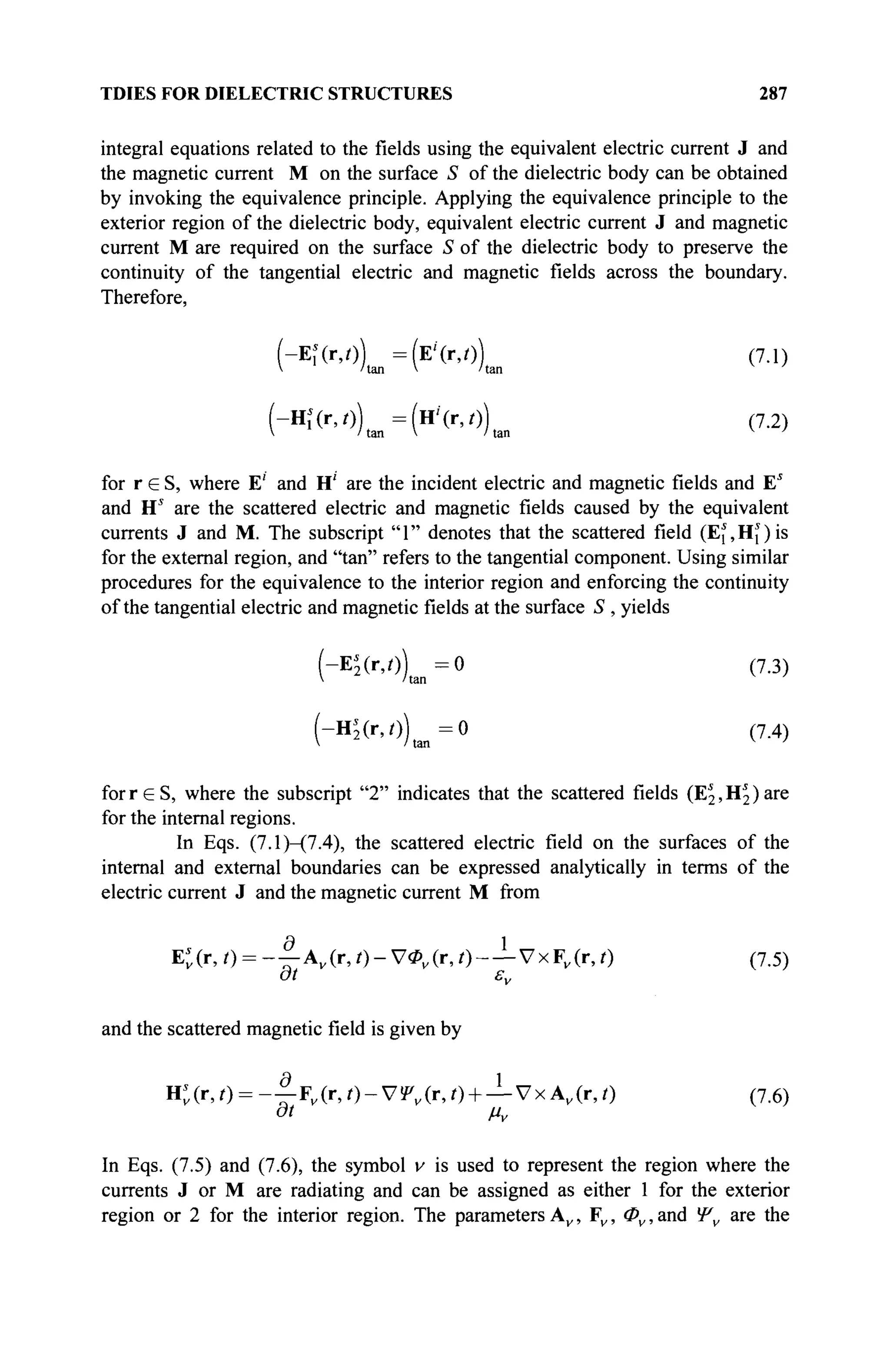
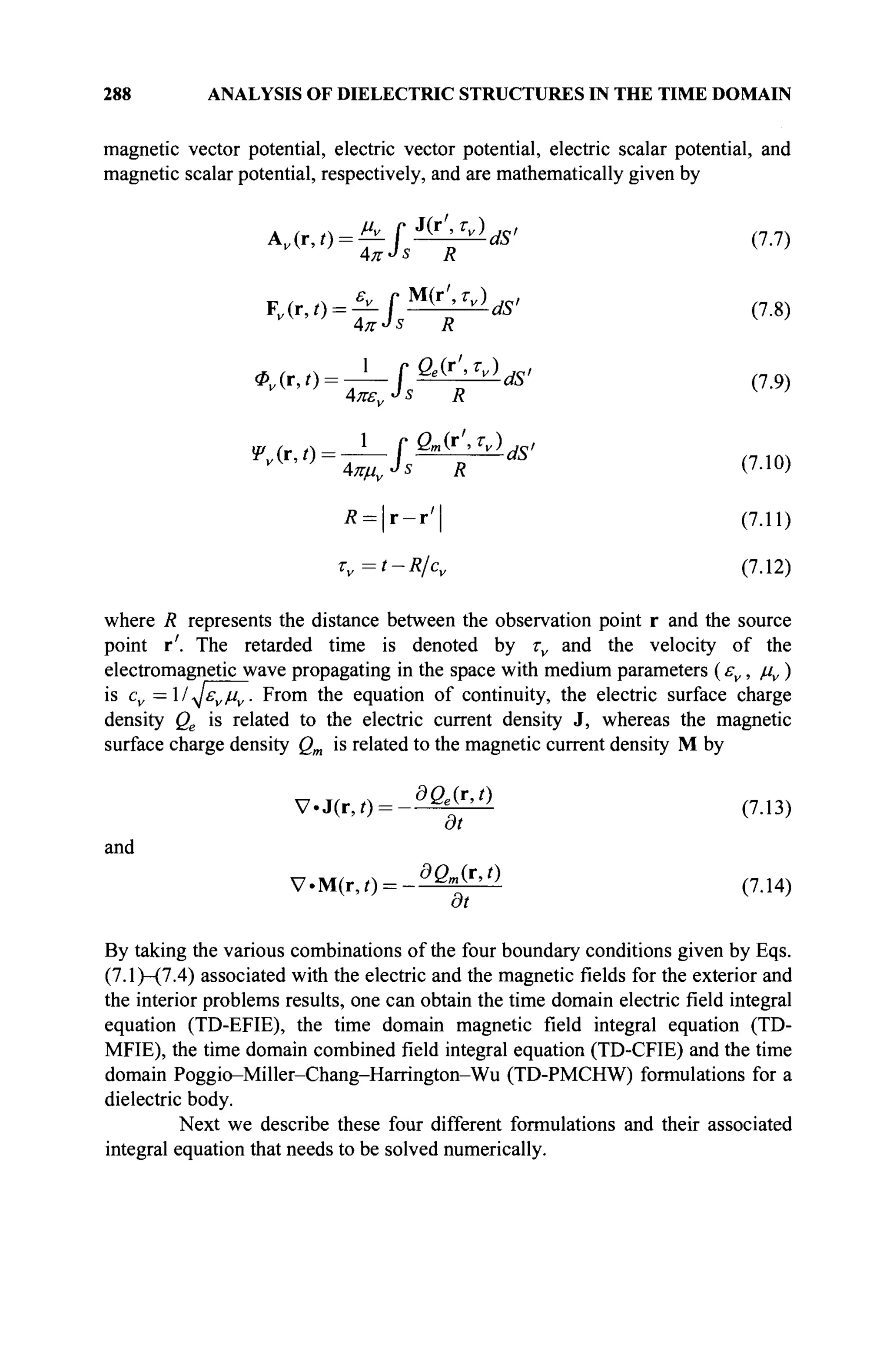
![TDIES FOR DIELECTRIC STRUCTURES 289
7.2.1 TD-EFIE
When combining the two boundary conditions of Eqs. (7.1) and (7.3) that are
related only to the electric field, the TD-EFIE is formed. It gives the relation in the
time domain between the incident electric field and the scattered electric field as a
result of the induced electric and magnetic currents. Further substituting the
expression for the scattered electric field given by Eq. (7.5), one obtains the TD-
EFIE as
Л 1
— Av(r,t) + V<Pv(r,t) + — VxF„(r,0
at ε„
ÎE'(r,0) , v = l
'tan
o, v = 2
(7.15)
7.2.2 TD-MFIE
Dual to the TD-EFIE formulation, the MFIE formulation is obtained by selecting
the two boundary conditions on the magnetic field only (i.e., using Eq. (7.2) and
Eq. (7.4)). Substituting the expression for the scattered magnetic field given by Eq.
(7.6), one obtains the TD-MFIE as
-f-F„(r, O + ViPUr, 0 - — Vx А„(г, О
(H''(r,0) , v = l
V Man
0, v = 2
(7.16)
7.2.3 TD-CFIE
By linearly combining the TD-EFIE of Eq. (7.15) and the TD-MFIE of Eq. (7.16),
the combined field integral equation is obtained as follows[15]:
(l-/r)(-Et(r,0) +JO7v(-Hj(r,0)
'tan 'tan
(l-*-)(E'(r,/)) +*77„(H'(r,0) , V = (7.17)
= 'tan 'tan
o, v = 2
where к is the usual combination parameter that can have any value between 0
and 1, and ην is the wave impedance of region v.
7.2.4 TD-PMCHW
An alternative way to combine the four equations given by Eqs. (7.1)—(7.4) yields
the PMCHW formulation. In this formulation, the set of four equations is reduced
to two by adding Eq. (7.1) to Eq. (7.3) and Eq. (7.2) to Eq. (7.4) to yield](https://image.slidesharecdn.com/timeandfrequencydomainsolutionsofemproblemsusingintegralequationsandahybridmethodologyb-250205130750-568a5ba2/75/Time-and-Frequency-Domain-Solutions-of-EM-Problems-Using-Integral-Equations-and-a-Hybrid-Methodology-B-H-Jung-pdf-310-2048.jpg)
![290 ANALYSIS OF DIELECTRIC STRUCTURES IN THE TIME DOMAIN
2
Σ
v = l
2
Σ
r 1
— A„(r,0 + V*„(r,/) + —VxF„(r,/)
at ε,,
| . F v ( r , 0 + V!P„(r,0-—VxAv (r,i)
(Е'(Г,О)
V /tai
(н'(г,о)
(7.18α)
(7.186)
7.3 SOLUTION OF THE TDIES BY USING THE MOD METHOD
Next, the solution of the TDIEs described in the previous section for a dielectric
structure is obtained by using the MOD method that has been introduced in
Chapters 5 and 6. In the MOD method, the surface of the dielectric structure is
approximated by planar triangular patches, and the triangular vector functions
called the RWG functions are used as the spatial basis and testing functions. The
triangular vector function f„ associated with the nth common edge is defined by
[16]
f„(r) = f„+
(r) + f„-(r)
tf(0
—— o^ r e r è
± P „ . rein
(7.19a)
(7.19è)
0, riit
where ln and An are the length of the edge n and the area of the triangle T*,
respectively. The position vector, p*, is defined with respect to the free vertex of
T^. For a dielectric body, another set of vector basis function g„ is required, and
it is defined by
where
g„(r) = nxf„(r)
g„(r) = g^(r) + g«(r)
g±(r) = nxfB
±
(r)
(7.20a)
(7.206)
(7.20c)
where n is the unit normal pointing outward from the surface at r. The functions
f„ and g„ are pointwise orthogonal within a pair of triangular patches.
7.3.1 Solving the TD-EFIE
7.3.1.1 Spatial Expansion and Testing. To solve the TD-EFIE for dielectric
structures given by Eq. (7.15), the electric current J and the magnetic current M](https://image.slidesharecdn.com/timeandfrequencydomainsolutionsofemproblemsusingintegralequationsandahybridmethodologyb-250205130750-568a5ba2/75/Time-and-Frequency-Domain-Solutions-of-EM-Problems-Using-Integral-Equations-and-a-Hybrid-Methodology-B-H-Jung-pdf-311-2048.jpg)
![SOLUTION OF THE TDIES BY USING THE MOD METHOD 291
on the dielectric structure first are approximated by the two spatial basis functions
as
N
J(r,0 = Xy„(0f„(r) (7.21α)
n=
N
M(r,0 = X)Ml l (0gB (r) (7.21ft)
n=
where Jn (t) and Mn (t) are the unknown coefficients to be determined and N is
the number of edges on the triangular patches approximating the surface of the
dielectric body. These basis functions also have been used in the frequency
domain formulation [17,18].
To handle the time derivative of the magnetic vector potential A(r,f) in
Eq. (7.15) analytically, the Hertz vector u(r, t) is introduced for the electric
current and is defined by
J(r,,) = ^ (7.22)
at
And the relation between the Hertz vector and the electric charge density is given
by
ße (r,0 = -V«u(r,0 (7.23)
Similarly, another Hertz vector related to the magnetic current is defined by
M(r,0 = ^ (7.24)
at
Using the basis function defined by Eq. (7.21), the Hertz vectors for the electric
and the magnetic currents are expressed as
u(r,0 = J>„(Of„(r) (7.25a)
и=1
N
v(r,i) = ^v„(Og„(r) (7.25b)
л=1
Therefore, the solution for the unknown current coefficients J„{t) and M„(t)
implies that one needs to determine un{t) and v„(f). The next step in the
numerical implementation is to develop a testing procedure to transform the
operator equation of Eq. (7.15) into a matrix equation using the method of moment](https://image.slidesharecdn.com/timeandfrequencydomainsolutionsofemproblemsusingintegralequationsandahybridmethodologyb-250205130750-568a5ba2/75/Time-and-Frequency-Domain-Solutions-of-EM-Problems-Using-Integral-Equations-and-a-Hybrid-Methodology-B-H-Jung-pdf-312-2048.jpg)
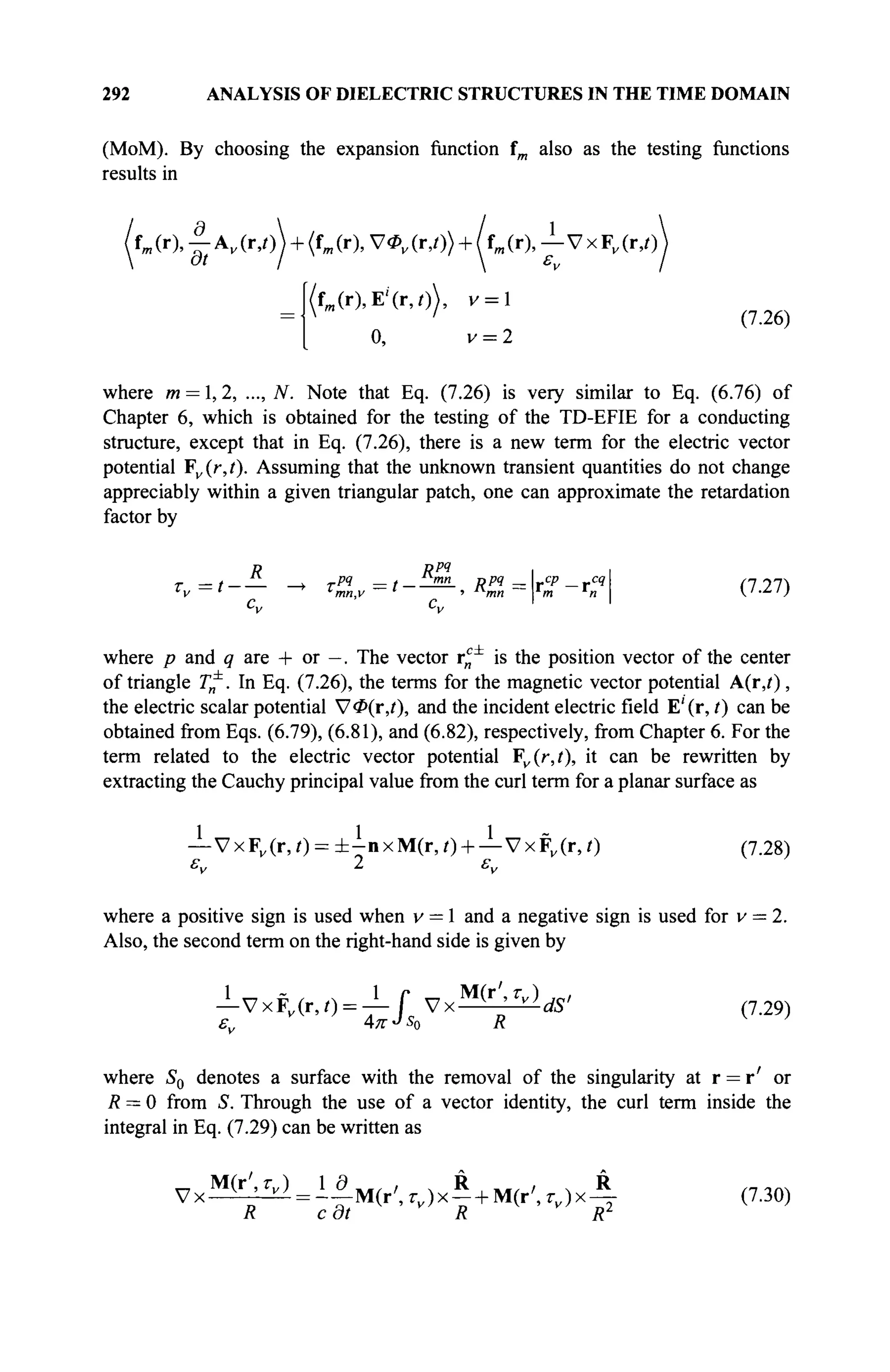
![SOLUTION OF THE TDIES BY USING THE MOD METHOD 293
where R is a unit vector along the direction r —r'. Thus, using Eq. (7.28), the
third term in Eq. (7.26) becomes
X ( r ) A v x F ^ r , o = /fm (r),±inxM(r,o + /fm (r),^-VxFF (r,i) ( ? 3 1 )
Substituting the magnetic current M(r,/) given by Eqs. (7.24) and the Hertz
vector v(r,i) given by (7.25b) into Eq. (7.31), the first term of the right-hand side
in Eq. (7.31) becomes
where
fm(r), ± i n x M ( r , 0 ) = Σ ς ^ ^-v„(t)
2
I „=i dt
r =.
mn,v
+Cmn, v =
~Cmn, v = 2
С = Υ^ Cpq
= C++
+ C+
+ C~+
4- С
Р.Ч
CZ=is^{r)-nxgl(r)dS
(7.32a)
(7.326)
(7.32c)
(7.32a)
where p and q can be either + or —. The integral of Eq. (7.32a) can be
computed analytically [19]. Using Eq. (7.29), the second term of the right-hand
side in Eq. (7.31) can be written as
fm (r),—VxFv (r,0) = E T - 1 Л « " Г
-^TV„(r„)gZ(r')x£
cv dt R
+ 4v„(r„)g2(r')x^-
dt Rz dS'dS (7.33)
By defining the retarded time by Eq. (7.27), one obtains
fm(r),— VxFv (r,0 (7.34α)
ΣΣ
л=1 p,q
where
Cm
И2
И
Су dt1
dt
^=i//^( r )
-/s8
«( r
') x
F^ (7.346)](https://image.slidesharecdn.com/timeandfrequencydomainsolutionsofemproblemsusingintegralequationsandahybridmethodologyb-250205130750-568a5ba2/75/Time-and-Frequency-Domain-Solutions-of-EM-Problems-Using-Integral-Equations-and-a-Hybrid-Methodology-B-H-Jung-pdf-314-2048.jpg)
![294 ANALYSIS OF DIELECTRIC STRUCTURES IN THE TIME DOMAIN
The integral in Eq. (7.346) may be evaluated using the Gaussian quadrature for the
unprimed and the primed coordinates numerically. Substituting Eqs. (7.32) and
(7.34) into Eq. (7.31), one obtains
fm(r), — VxF„(r,0
=Σ at
PA
£pq
d2
rl
Z J _ Ü _ V (ТРЧ + ГРЧ _ v (ТРЧ
cv dt dt
(7.35)
Lastly, substituting Eq (7.33) into Eq. (7.24) along with Eqs. (6.79), (6.81), and
(6.82) of Chapter 6, one obtains
Σ Σ
n= p,q
и ,pq
ti (трч
I "mn
v (rpq
Л
dtL
BP4
£„ л=1 " '
+ΣΣ
«=1 PA
where
Д
( ГРЧ ^ fj
2 J _ _ V (rpq
4-rpq
—v (rpq
,2 v
nT
mn,v)^h2 .v
nT
mn,v)
Cv dt dt
AZ=— f£(r). f ^^-dS'dS
УЧУ) v
= K(0 (7.36a)
РЧ
--.-fr-wlr^1
*
4π·
dS
CZ=lfX(r)-nxgq
„{r)dS
vv
m{t).
fsfm(r).Ei
(r,t)dS, v =
0, v = 2
(736b)
(7.36c)
(7.3&0
(7.36e)
(7.36/)
7.3.1.2 Temporal Expansion and Testing. Now, consider the choice of the
temporal basis function and the temporal testing function. An orthonormal basis
function set derived from the Laguerre polynomials called the associated Laguerre
functions can be written as [11]
0,(0 = *"'%(') (7.37)](https://image.slidesharecdn.com/timeandfrequencydomainsolutionsofemproblemsusingintegralequationsandahybridmethodologyb-250205130750-568a5ba2/75/Time-and-Frequency-Domain-Solutions-of-EM-Problems-Using-Integral-Equations-and-a-Hybrid-Methodology-B-H-Jung-pdf-315-2048.jpg)
![SOLUTION OF THE TDIES BY USING THE MOD METHOD 295
The coefficients for the temporal expansion functions un{t) and vn{t) introduced
in Eqs. (7.25a) and (7.25b), which are assumed to be causal responses (i.e., exist
only for t > 0 ) can be expanded using Eq. (7.37) as
"я(0 = ХХу^(аО
7=0
(7.38α)
v
»(0 = Ëv
»J*/(s
') (7.38b)
where un ■ and v · are the fixed coefficients to be determined, and 5 is a scaling
factor. Applying the derivative property of the associated Laguerre functions given
in the appendix of Chapter 5 [20-22], the first and second derivatives of un(t) can
be written explicitly in terms of the time domain coefficient и · as [20]
d °° ί 1 •/
'~1
dt 7=0
Φ^ί)
dtz
7=0
У-1
-jun(t) = s2
Y^ -unj+^2(j-k)unk
*=0
Φ^ή
Similarly, the first and the second derivatives of vn (t) are given as
"' 7=0 I Z
k=0
dt'
oo < j 7-1
7=0
^y(s/)
(7.39a)
(7.396)
(7.40a)
(7.40b)
In deriving these expressions, it has been assumed that both the function and its
first derivative are zero at / = 0 because of causality. Substituting Eqs. (7.38)-
(7.40) into the spatial testing of Eq. (7.36) and performing a temporal testing,
which means multiplying by $(sf) and integrating from zero to infinity, one
obtains](https://image.slidesharecdn.com/timeandfrequencydomainsolutionsofemproblemsusingintegralequationsandahybridmethodologyb-250205130750-568a5ba2/75/Time-and-Frequency-Domain-Solutions-of-EM-Problems-Using-Integral-Equations-and-a-Hybrid-Methodology-B-H-Jung-pdf-316-2048.jpg)
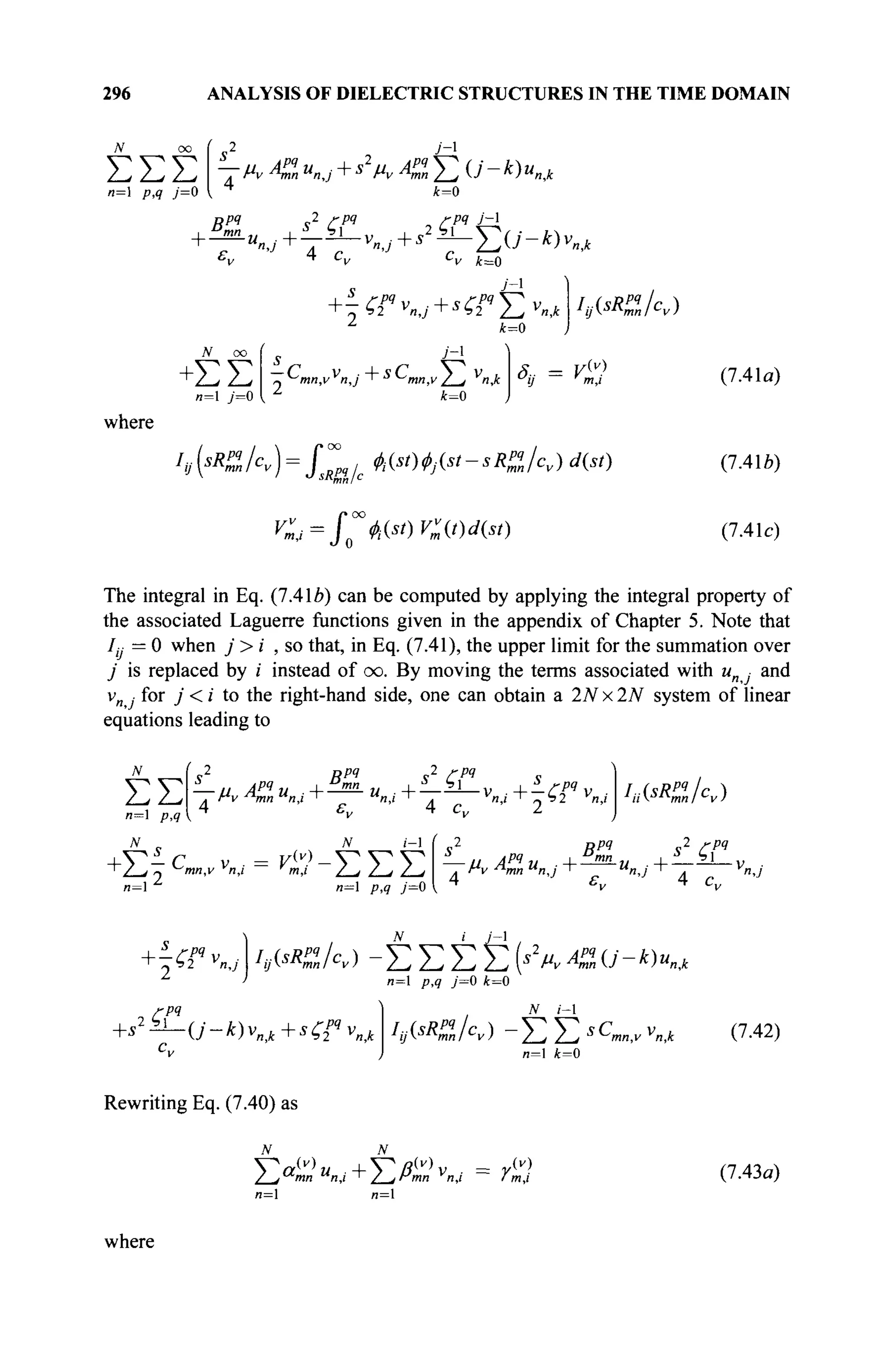
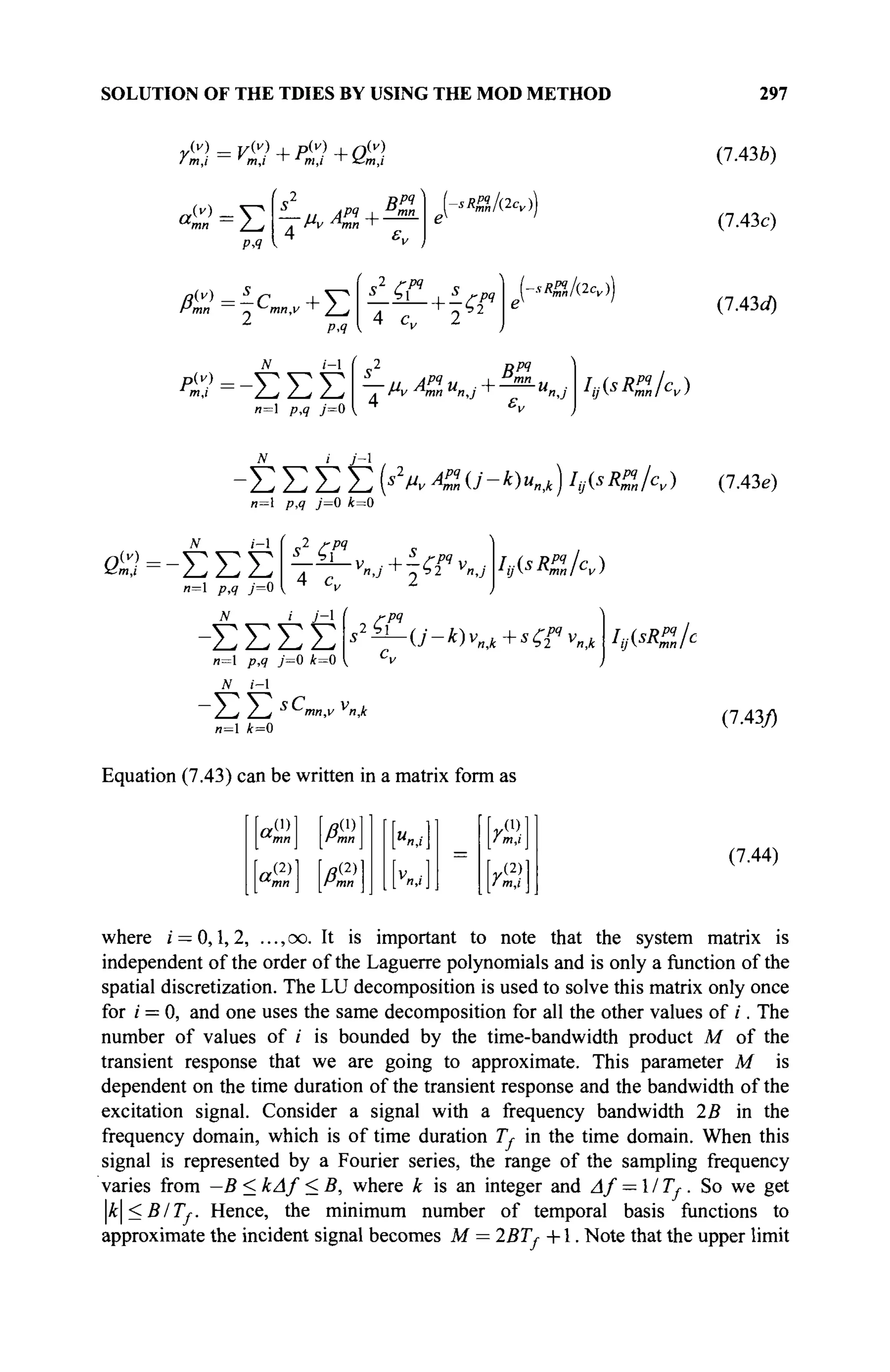
![298 ANALYSIS OF DIELECTRIC STRUCTURES IN THE TIME DOMAIN
of the integral V„j in Eq. (7.41c) can be replaced by the time duration sTj- instead
of infinity.
An implicit MOT method also will have similar computational
operations. However, at stage / = 0 for the implicit MOT method, one will be
solving a sparse matrix instead of a dense one. In addition to the number of
timesteps at which the implicit MOT scheme solves the problem, at each timestep
either is related to the rise time of the pulse or related to the spatial discretizations
determined by the Courant condition. Typically, the spatial discretization requires
at least 10 subsections per wavelength. The timestep is determined by this spatial
discretization divided by the velocity of light. The Courant condition instead of the
rise time of the incident pulse will dictate the value for the timestep. For the MOD
method, however, the solution needs to be computed at a total number of M steps,
which is determined by the time bandwidth product of the waveform, which is
generally much smaller than the number of timesteps for an implicit MOT scheme.
7.3.1.3 Computation of the Scattered Far Field. By solving Eq. (7.44), using a
LU decomposition, in a marching-on-in-degree manner with M temporal basis
functions, the Hertz vector coefficients unj- and vn · are obtained. Then, the
electric and magnetic current coefficients Jn (?) and Mn (t) can be expressed using
Eqs. (7.22) and (7.24), Eqs. (7.25a) and (7.25Z>) with Eqs. (7.39a) and (7.40a),
respectively, resulting in
Q M-
л(о=-^-и|1(о =SJ2
0 t
y=0
1 J
~]
Z
k=0
g м- j j -
a t
j=0 { L
k=0
</>j{st)
ΦΜ).
(7.45a)
(7.45b)
Once the equivalent currents on the dielectric structure have been determined, the
far scattered fields can be computed. These fields may be thought as the
superposition of the fields separately produced by only the electric and the
magnetic currents. The analytical form of the far fields can be derived directly
from the transient coefficients un (t) and vn (t), which can be obtained by solving
Eq. (7.44) with Eq. (7.38). The scattered field caused by the electric currents alone
at a point r is given by
Ei(r,0<
ЭА(г,р
dt
(7.46)
where the subscript J refers to the electric current. Substituting Eqs. (7.7), (7.22),
and (7.25a) into Eq. (7.46) along with Eq. (7.19a) results in](https://image.slidesharecdn.com/timeandfrequencydomainsolutionsofemproblemsusingintegralequationsandahybridmethodologyb-250205130750-568a5ba2/75/Time-and-Frequency-Domain-Solutions-of-EM-Problems-Using-Integral-Equations-and-a-Hybrid-Methodology-B-H-Jung-pdf-319-2048.jpg)
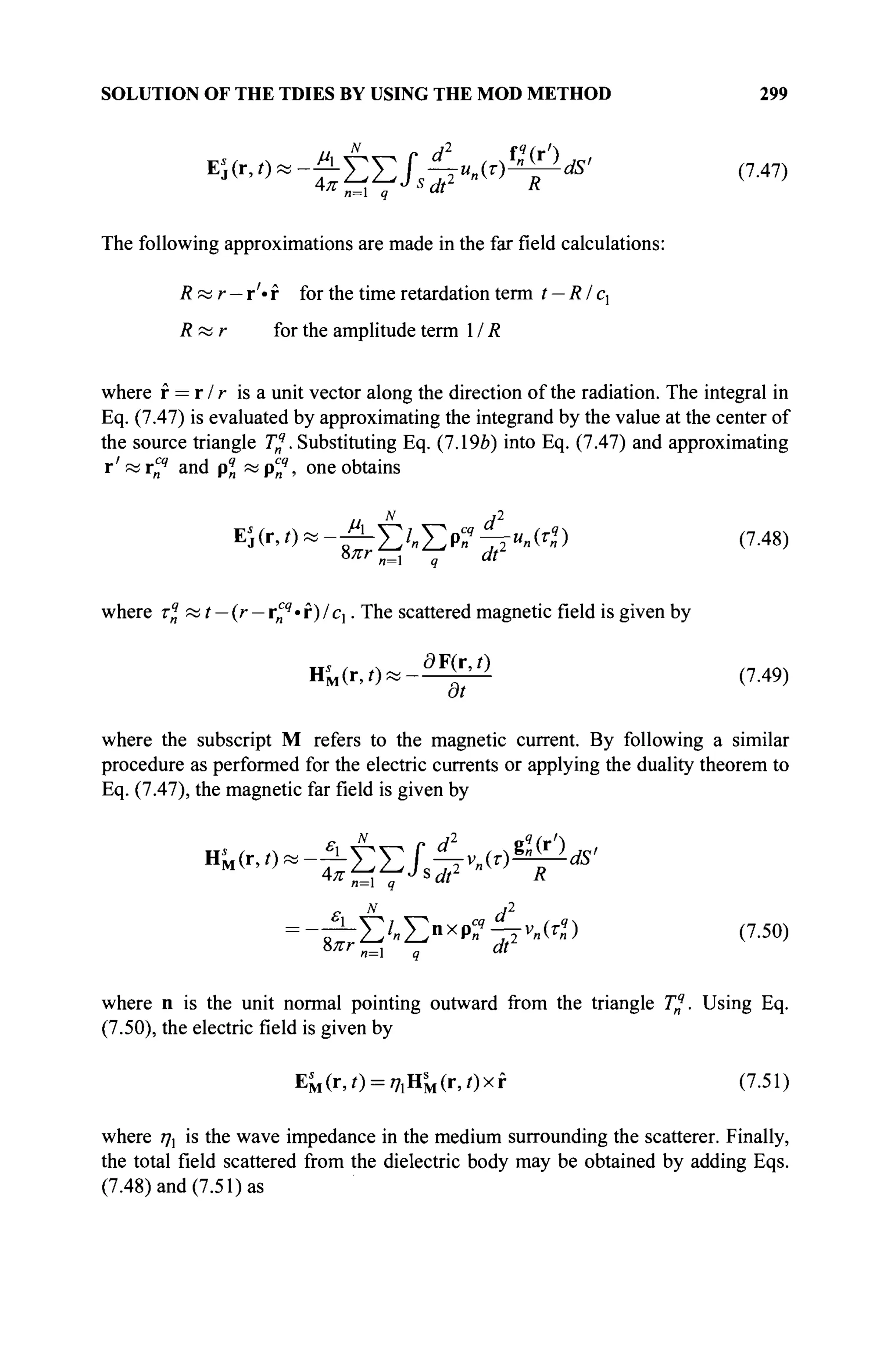
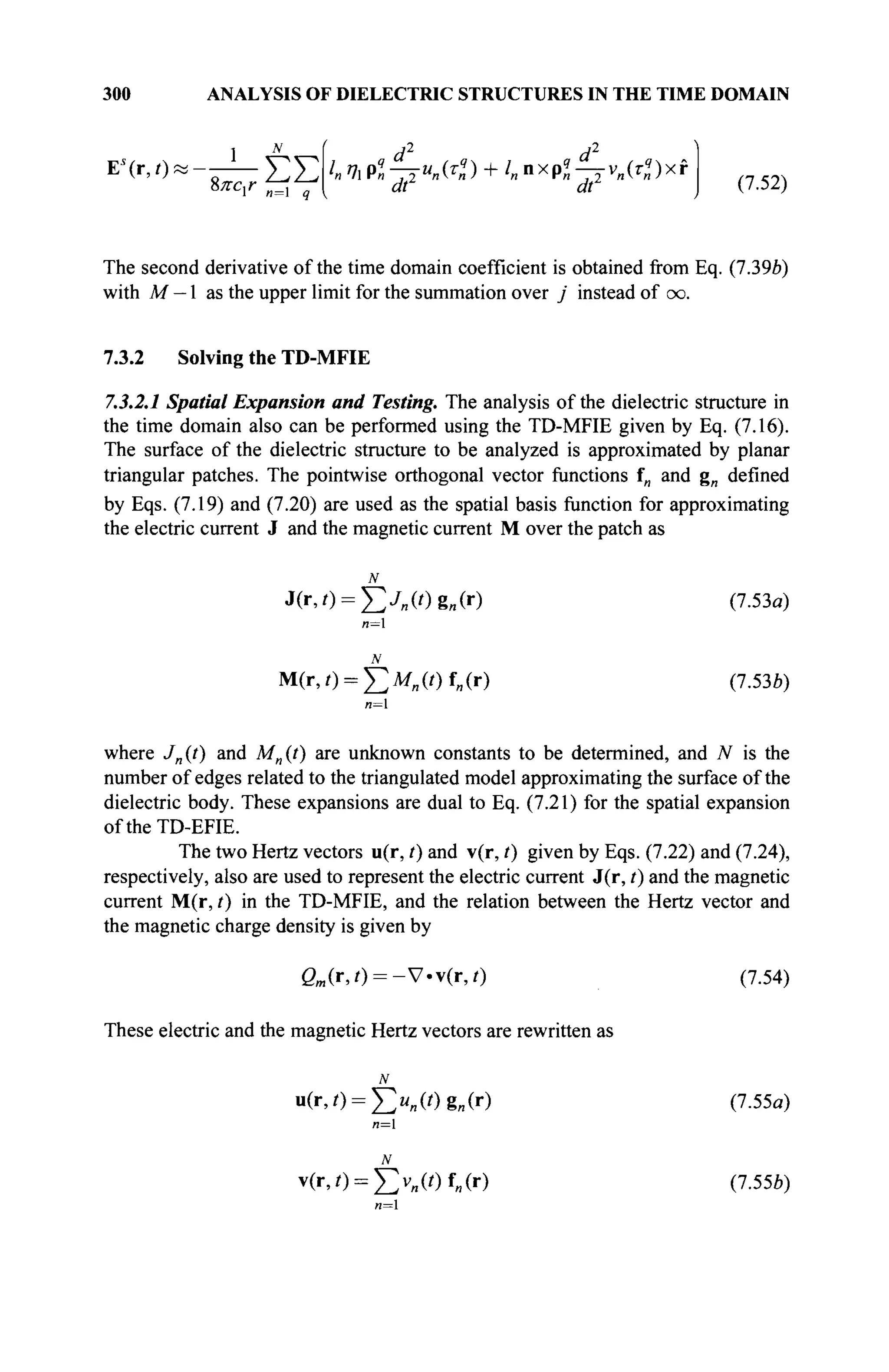
![SOLUTION OF THE TDIES BY USING THE MOD METHOD 301
By choosing the expansion function fm also as a testing function, the testing of the
TD-MFIE yields
/fm (r),^Fv (r,/)J + (fm(r), V!P„(r,/))-ltm (r), — Vx A,(r, t)
(fm (r),H4r,0), v = l
0, v = 2 (7
·56
)
where m = 1, 2, ..., N. The next step in the MoM procedure is to substitute the
expansion functions of the Hertz vectors defined in Eqs. (7.55) into Eq. (7.56).
First consider the testing of the integral related to the electric vector potential
F(r, /). Using Eqs. (7.8), (7.53Й), and (7.55b), results in
(ur),ftK(r,t)) = t f~JsW .f^rj-ψ dS'dS (7.57)
Assuming that the unknown transient quantity does not change appreciably within
the triangular patch as in Eq. (7.27), Eq. (7.57) can be written as
fm (r),|;F,(M)) = Σ Σ evAZ~vnitZy) (7.58a)
0 t
I B=l p,q "t
where
^—JfiV.f^ds'ds (7.58*)
Next consider the testing of the gradient of the scalar potential Ψ(τ, t) in Eq.
(7.57). Using the vector identity V-УА = A - V f + f V - A and the property of
the spatial basis function [16], one can write
<fm (r), V Ψν (r, 0} = -fs V · f
m (r) ψν (r, 0 dS
= Στ^JУ-WJ(Tv)^^-dS>dS (7.59)
With the assumption for the retarded time given by Eq. (7.27), Eq. (7.59) can be
written as
N fypq
{ fm(r), V!P„(r, 0 > = Σ Σ —ν
Λ<1,ν) (7.60α)
n= p,q f*v](https://image.slidesharecdn.com/timeandfrequencydomainsolutionsofemproblemsusingintegralequationsandahybridmethodologyb-250205130750-568a5ba2/75/Time-and-Frequency-Domain-Solutions-of-EM-Problems-Using-Integral-Equations-and-a-Hybrid-Methodology-B-H-Jung-pdf-322-2048.jpg)
![302 ANALYSIS OF DIELECTRIC STRUCTURES IN THE TIME DOMAIN
where
B%=±fsV-fr(r)fs^^ldS'dS (7.60b)
The integrals in Eqs. (7.58Й) and (7.60b) may be evaluated by the method
described in Ref. [16]. Extracting the Cauchy principal value from the curl term
for a planar surface, the third term of Eq. (7.56) for the testing of magnetic vector
potential A(r, t) may be written as
—VxAv (r,i) = ± - n x J + — VxA„(r,0 (7.61)
where the positive sign is used when v = 1 and the negative sign is used for
v = 2. The second term of the right-hand side in Eq. (7.61) is given by
-VxÀv (r,0 = - î - f V x ^ b d d S ' (7.62)
4nJs0 R v
'
where S0 denotes the surface with the removal of the contribution due to the
singularity at r = r' or R — 0 from the surface S. Using a vector identity [23],
the curl term inside the integral in Eq. (7.62) is given by
J(r',rv) 1 9 ¥ / , ч R л, , ч R
Vx ; r -i
^ = -—J(r',î-V )x —+ J(r',r„)x— (7.63)
where R is a unit vector along the direction r —r'. Thus, using Eq. (7.61), the
third term in Eq. (7.56) becomes
/fm (r),— V x A , ( r , / ) = / f m ( r ) , ± ^ n x j + /fm (r),— Vx„(r,/) (7.64)
Now, consider the first term in the right-hand side of Eq. (7.64). Substituting the
Hertz vector u(r,i) in terms of the electric current J(r,/) of Eqs. (7.22) and
expanding the Hertz vector u(r,i) using (7.55a) yields
1 N
d
f « ( r ) , ± - n x J ) = YtCmntV—un{t) (7.65a)
where
B=i dt
C
m„,v - 1 r , (7.65b)](https://image.slidesharecdn.com/timeandfrequencydomainsolutionsofemproblemsusingintegralequationsandahybridmethodologyb-250205130750-568a5ba2/75/Time-and-Frequency-Domain-Solutions-of-EM-Problems-Using-Integral-Equations-and-a-Hybrid-Methodology-B-H-Jung-pdf-323-2048.jpg)
![SOLUTION OF THE TDIES BY USING THE MOD METHOD 303
с = V c w
= c++
+c+
~ + c-+
+ c~ (7.65c)
(7.65a)
The integral of Eq. (1.65d) can be computed analytically [19]. Using Eq. (7.63),
the second term on the right-hand side in Eq. (7.64) becomes
fm (r),—VхАДг,/)) = £ - L J fm(r). f
So
d „ / R
ju„{Tv)gq
„{r)x —
cv dt R
d R
—"„(^)g«(r
')x-j
ai R
dS'dS (7.66)
By approximating the retarded time as in Eq. (7.27), one obtains
fm (r),—νχΑ,(ιν)) = έ Σ
f*v I n= p,q
£pq
d2
d
cv dt1
dt
(7.67a)
where
^ = ^ / / ™ ( r )
- / s g
« ( r
' ) x
F ^ (7.67*)
The integral in Eq. {1.61b) may be evaluated using the Gaussian quadrature
numerically for the unprimed and the primed coordinates. Substituting Eqs. (7.65)
and (7.67) into Eq. (7.64), one obtains
U r ) , - j - V x A v ( r , 0 = Y^C^ jua(t)
л=1
+ΣΣ
n= p,q
ГРЧ j 2
^ ' ,, (TPI Л-1_/-РЧ^_,. (Tpq
d_
dt
cv dt
Finally, substituting Eqs. (7.58), (7.60), and (7.68) into Eq. (7.56), one obtains
(7.68)
ΣΣ
и=1 p,q
F ЛРЧ ϋ _ υ (ТРЧ | "mn / pq
c
v ^τηη ,2 v
nL
mn,v>~ __ v
ni
mn,v)
ВРЧ
dt μν
N ( ζ η d2
Y^C
mn*-Zu
n(f)
^ί dt
-ΣΣ
и=1 p,q
cv dt1
u
n(T
mn,v) + hl , u
nT
mn,v) Vv
m(t) (1.69a)](https://image.slidesharecdn.com/timeandfrequencydomainsolutionsofemproblemsusingintegralequationsandahybridmethodologyb-250205130750-568a5ba2/75/Time-and-Frequency-Domain-Solutions-of-EM-Problems-Using-Integral-Equations-and-a-Hybrid-Methodology-B-H-Jung-pdf-324-2048.jpg)
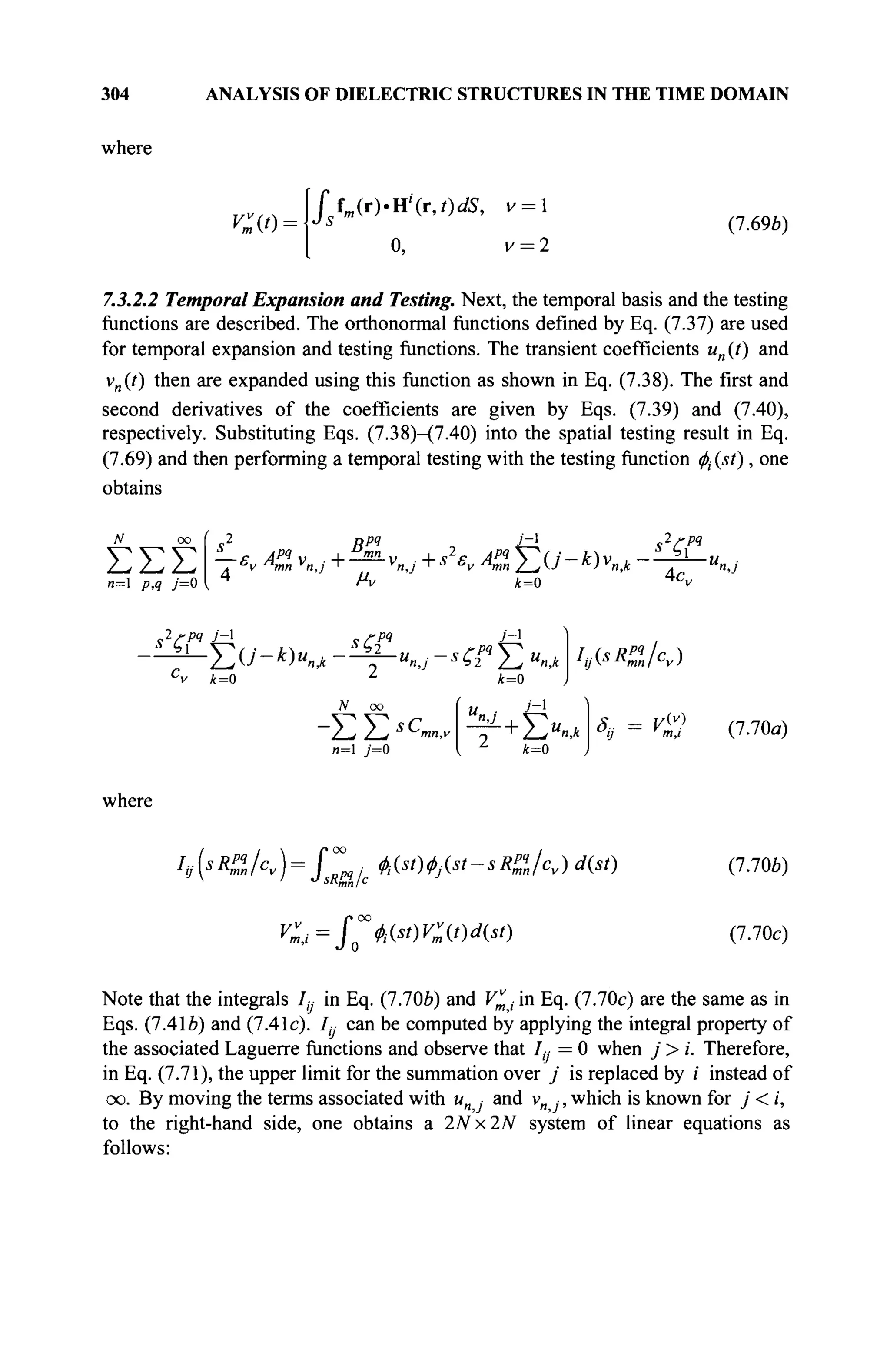
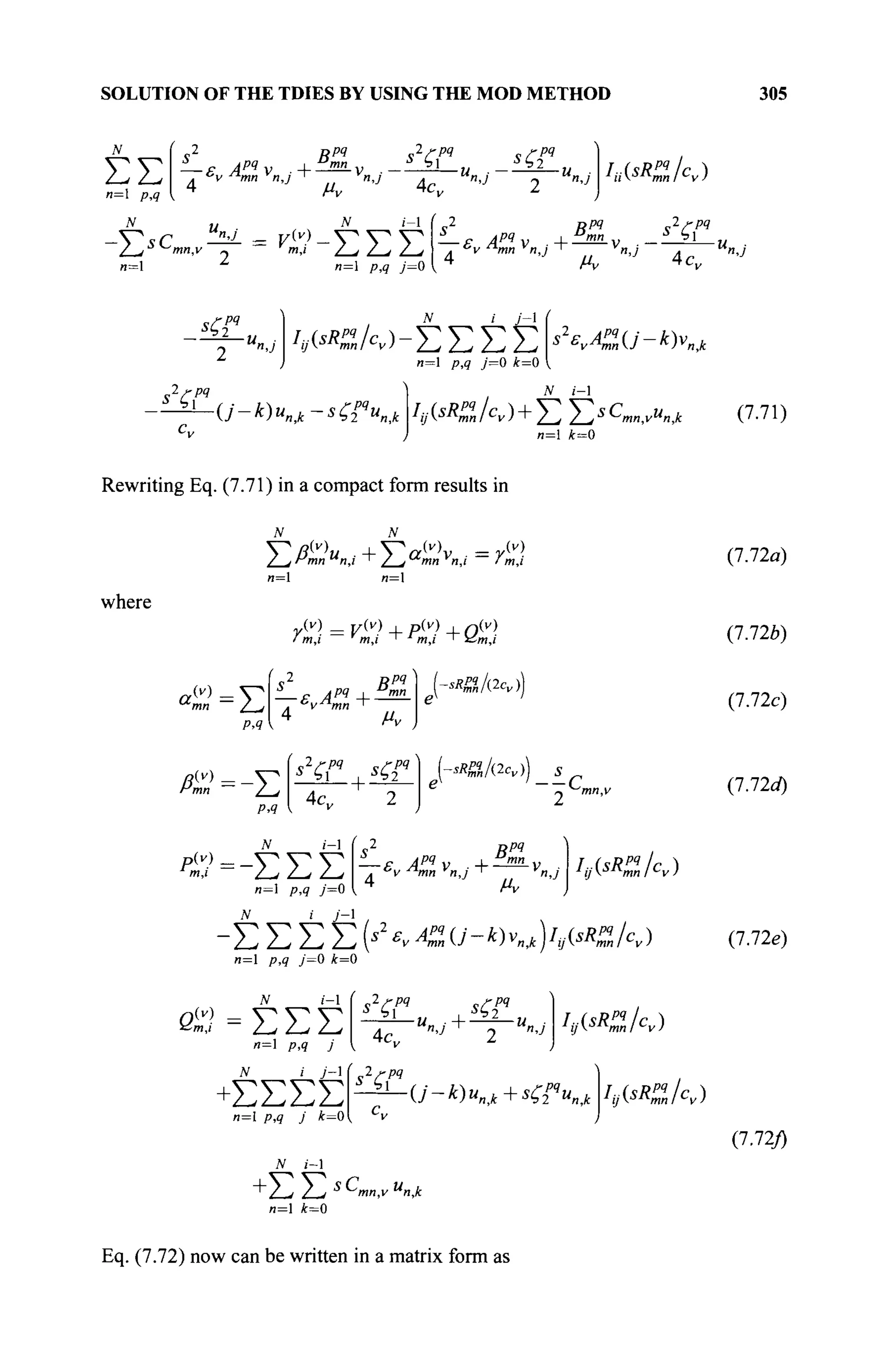
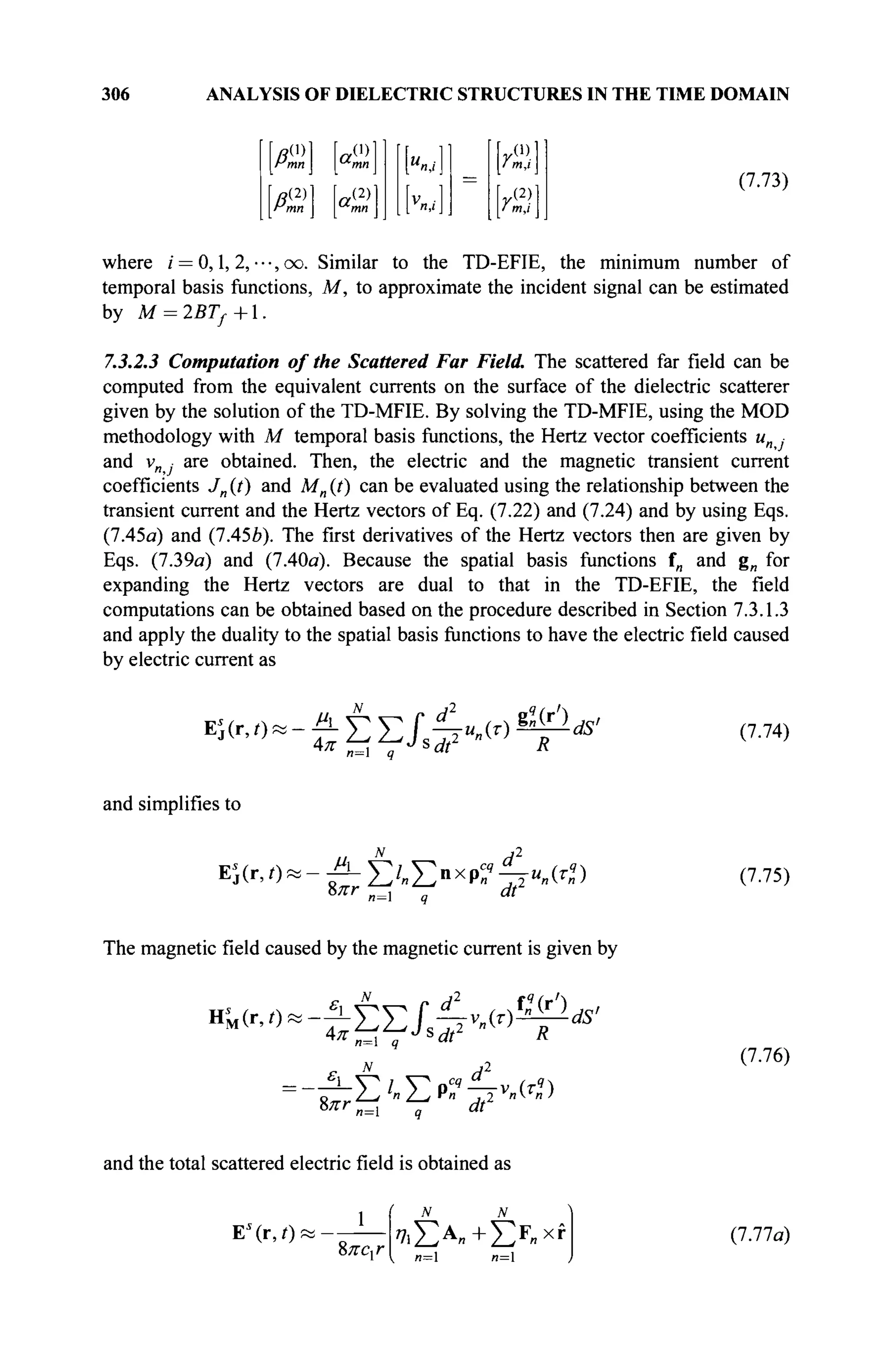
![SOLUTION OF THE TDIES BY USING THE MOD METHOD 307
.2
" "^ Vn
dt2
(7.776)
.2
Ρ « = ^ Σ Ρ " Τ Τ ν
» ( Γ
« ) (7.77c)
7.3.3 Solving the TD-CFIE
7.3.3.1 Spatial Expansion and Testing. To solve TD-CFIE of Eq. (7.15), the
electric and the magnetic currents are approximated by the functions f„ defined in
Eq. (7.17), resulting in
j(r,o=E^wf„(r) (778a)
M(r,/) = f i i , ( / ) f , ( r ) (7.786)
и=1
The Hertz vectors u(r,t) and v(r,i) defined in Eqs. (7.22) and (7.24) are used and
are given by
u(r,/) = £)i/e (0f„(r) (7.79α)
4.
"i
N
v(r,r) = £ > „ ( / ) f„(r) (7.796)
/ 7 = 1
Similar to the testing of the CFIE in the frequency domain presented in section 3.6
[15], the spatial testing of TD-CFIE formulation uses a combination of f„ and its
orthogonal vector g„ as the testing functions to convert the TD-CFIE into a
matrix equation. A general expression for the spatial testing of TD-CFIE using the
four parameters, fE, gE, fH, and gH, in conjunction with the testing functions
f„ and g„ may be written as
(l-K)(fEtm+gEgm,-Es
v(r,t)) + wv(fHfm+gHgm,-lls
v(r,t)) =
(l-K)(fEfm+gEgm,Ei
(r,t)) + >c^(fHL+gHem,'ai
(r,t)) for v =
0 v = 2 (7
-8
°)](https://image.slidesharecdn.com/timeandfrequencydomainsolutionsofemproblemsusingintegralequationsandahybridmethodologyb-250205130750-568a5ba2/75/Time-and-Frequency-Domain-Solutions-of-EM-Problems-Using-Integral-Equations-and-a-Hybrid-Methodology-B-H-Jung-pdf-328-2048.jpg)
![308 ANALYSIS OF DIELECTRIC STRUCTURES IN THE TIME DOMAIN
where m = ,2,---,N and the testing coefficients fE, gE, fH, and gH, may be
+ 1 or — 1. This equation is termed as the TENE-THNH formulation as in Ref.
[14]. To simplify the transformation of Eq. (7.80) into a matrix equation, the
testing procedure is separated into two steps that are valid only for those terms
related to either the electric field or the magnetic field.
First, the portion related to only the electric field is tested with the testing
function fEîm + gEgm, and assuming that the transient quantities do not change
appreciably within a given triangular patch as in Eq. (7.27), result in
ΣΣ
и=1 p,q
,, Apq
— и (rpq
~>-
Hv^hnn , 2 n mn.v)
at
ррч
„ (τΡ4 +
Gpq
d
cvsv dt
и (трч
)
Dpq
d2
d
+ ^mn " ( Pq , F p q ^ _ v (Tpq
cv dr dt
+i2CmnAvn{t) = V^t)
„=i dt
(7.81)
Equation (7.81) is called the TENE formulation [14]. The expressions for the
coefficients A%, Fpq
, GZ, Cmn<v, DP
Z, and £ « , and V?v
t) are given by
Eqs. (7.A1)-(7.A6) and (7.A24) in the appendix at the end of this chapter.
7.3.3.2 Temporal Expansion and Testing. For the temporal testing of the TENE
formulation, the functions ^-(/) given by Eq. (7.37) are used. Using Eqs. (7.38)-
(7.40) in Eq. (7.81) and performing a temporal testing with the testing function
<f>i{st), one obtains
л
тп
1ССГ'I ß,
a,
£(2)
mn
QE(2)
mn
γΕ(λ)
i m,i |
rE(2)
]
/ m,i
(7.82a)
where
E(y) _ yE(v) , pE(y) , nE(v)
m,i m,i ' m,i ~ z£m,i
a,
E(v).
Έ
Р.Я
1
s2
u A?4
Fpq
sGpq
J
Hv^hnn , * mn , äKJ
mn
2c„s„
-sRffJ(2cv)
(7.82b)
(7.82c)
/e^^+E
! 42
npq
ч Fpq
л
^mn i л
^тп
4c„
sRffJdcA
V%v)
=f"WW?v
t)d(st)
(7.82c/)
(7.82e)](https://image.slidesharecdn.com/timeandfrequencydomainsolutionsofemproblemsusingintegralequationsandahybridmethodologyb-250205130750-568a5ba2/75/Time-and-Frequency-Domain-Solutions-of-EM-Problems-Using-Integral-Equations-and-a-Hybrid-Methodology-B-H-Jung-pdf-329-2048.jpg)
![SOLUTION OF THE TDIES BY USING THE MOD METHOD 309
n— p,q j—0
su Apq
Fpq
s G
^ ν -^^-^^v
JV / y'-l
+ΣΣΣΣ
n=l p,9 7=0 *=0
s2
MvApq
n(j-k)-
sGH
K,k hj(sR
mllc
v) (7.82/)
i - l
n—1 /7,^ у—О
tf i У-1
-ΣΣΣΣ
n=l p,9 y=0 i = 0
f с2
П И с f W
4c„
fi2
AÏÏ
VnjhjisRZhv)
t i - ^ V + ^ m » ^ hAsR
Zlcv)
и=1 A=0
'(, « A, ) = Φ,-j « к ) - й-y-i « /с, ), У < i
(7.82g)
(7.82A)
Following a similar procedure for the testing of the part only related to
the magnetic field in the TD-CFIE, a matrix equation can be written in which
/н^т+Вн%т is u s e
d as the spatial testing function and ^(/)is the temporal
basis function. This equation is termed the THNH formulation [14], where
,Я(2) Я(2)
mn mn
YH(X)
*m,i I
YH(2)
ί m,i
,H{v) _ yH{v) , pH{v) ,nH(v)
m,i m,i ' тл ' -&m,/
a,
H(v) _
Σ
PA
( 92
P / i w
F « чПРЧ
J с
у я
/ и л , J
mn ι и
ш
Pmn _ / J
z
p,q
ß v 1ενμν
S
Pmn i S
^mn
4c„
-sRff„klcv))
sRff„/(2cv))
C=-EEE
n=l p,q j=0
N i j -
-ΣΣΣΣ
n=l p,q j=0 k=0
VZP=$~b{st)V?v
t)d{st)
'njhjisRZhy)
v^IijisRZhy)
(7.83a)
(7.83è)
(7.83c)
(7.83rf)
(7.83e)
i_1
is2
e Apq
Fpq
sGpq
•*v -"-mn i ' mn
4 /"и 2ονμν
s'£vA%(j-k) +
>Gm„
С
УМУ )
(7.83/)](https://image.slidesharecdn.com/timeandfrequencydomainsolutionsofemproblemsusingintegralequationsandahybridmethodologyb-250205130750-568a5ba2/75/Time-and-Frequency-Domain-Solutions-of-EM-Problems-Using-Integral-Equations-and-a-Hybrid-Methodology-B-H-Jung-pdf-330-2048.jpg)
![310 ANALYSIS OF DIELECTRIC STRUCTURES IN THE TIME DOMAIN
β,Τ=ΣΣΣ
n=1
P.? У=0
N i j -
+ΣΣΣΣ
n= p,q j=0 k=0
4c„ 2
D,РЧ
N i - l
-{j-k) + sE% (7.83g)
+ Z-i i-j S
Cmn,v u
n,k
n= i=0
In Eq. (7.83), the elements A%, F%, G%, Cmn,v, D%, E%, and ^ ' ( 0 are
given by Eqs. (7.A7)-(7.A12) and (7.A25) as described in the appendix. The
matrix equations of Eqs. (7.82) and (7.83) can be written as
"LI W
«J] im.i
«mJ K i l = УтЛ
(7.84a)
(7.84b)
where wni =uni for n=, 2, ...,N and w„ ■ —vnj for n=N + ], 2, ...,2N.
Finally, a general matrix equation for the TD-CFIE can be obtained by
combining the TENE and THNH formulations given by Eqs. (7.84a) and (7.846)
as
a
mn ] [%,/ ] = Ут4 ]> i = 0, 1, 2, · · ·, OO (7.85α)
where
a„ Α-κ)αξ,„+κηνα%η
rm,i=(}-K)Yi,i+KlvYm,i
(7.85ft)
(7.85c)
By solving the matrix equations Eq. (7.85) using MOD with M temporal basis
functions, one obtains first the coefficients un, and v„,. Then the electric and the
magnetic current coefficients are derived using the relations in Eqs. (7.78)-(7.79)
and Eq. (7.38) [13].
7.3.3.3 Computation of the Scattered Far Field. Once the equivalent currents on
the dielectric scatterer have been determined using the TD-CFIE, the far scattered
fields can be computed. These fields may be thought of as the superposition of the
fields caused by the electric and magnetic currents obtained from the solutions of
TD-EFIE and TD-MFIE of Eqs. (7.44) and (7.73). Also, when we consider a
signal with time duration 7V in the time domain, we note that the upper limit of
the integral in Eqs. (7.82e) and (7.83e) can be replaced by the time duration sT,
instead of infinity.](https://image.slidesharecdn.com/timeandfrequencydomainsolutionsofemproblemsusingintegralequationsandahybridmethodologyb-250205130750-568a5ba2/75/Time-and-Frequency-Domain-Solutions-of-EM-Problems-Using-Integral-Equations-and-a-Hybrid-Methodology-B-H-Jung-pdf-331-2048.jpg)
![SOLUTION OF THE TDIES BY USING THE MOD METHOD 311
7.3.4 Solving the TD-PMCHW
7.3.4.1 Spatial Expansion and Testing. To solve the TD-PMCHW given by Eq.
(7.18), the electric and the magnetic currents are expanded by the triangular vector
function fn as shown in Eq. (7.78). The Hertz vectors u(r,t) and v(r,t) defined
in Eqs. (7.22) and (7.24) are used to substitute the electric current J(r, t) and the
magnetic currents M(r, t), and they are expanded by the spatial basis function f„
as in Eq. (7.79).
Consider the first equation Eq. (7.18a) of the TD-PMCHW formulation,
which relates to the electric field only. Substituting the expression of the electric
and magnetic Hertz vectors into Eq. (7.18a) and testing with the spatial functions
f
m results in
2 N
ΣΣΣ
v= n= p,q k
d2
Bpq
и API-—и irPI I mn
и (τΡΊ Λ
dt1
ε,,
Cpq
d2
d
.Ь] if_„ (ТРЯ ГРЧ л
cv dr dt
V*(t),m = ,2,-Jf (7.86α)
where
A»=±fst>ir).fsW£ldS'dS (7.86b)
B% ~fsV«?)fs ^''^dS'dS (7.86c)
# " = 7 - fjm(r> fX(r')x^dS'dS,k = l,2 (7.86a)
V*{t) = jsim{r).¥l(r,t)dS (7Me)
Note that Eq. (7.86) is very similar to the spatial testing result obtained for the TD-
EFIEofEq. (7.36).
7.3.4.2 Temporal Expansion and Testing. Using the temporal basis function
φj(st) defined by Eq. (7.37) to approximate the transient coefficients of Eq. (7.86)
and performing a temporal testing with the testing function $(ίί), one obtains
T(aE
и +ßE
v ) = rE
. (7.87α)
where](https://image.slidesharecdn.com/timeandfrequencydomainsolutionsofemproblemsusingintegralequationsandahybridmethodologyb-250205130750-568a5ba2/75/Time-and-Frequency-Domain-Solutions-of-EM-Problems-Using-Integral-Equations-and-a-Hybrid-Methodology-B-H-Jung-pdf-332-2048.jpg)
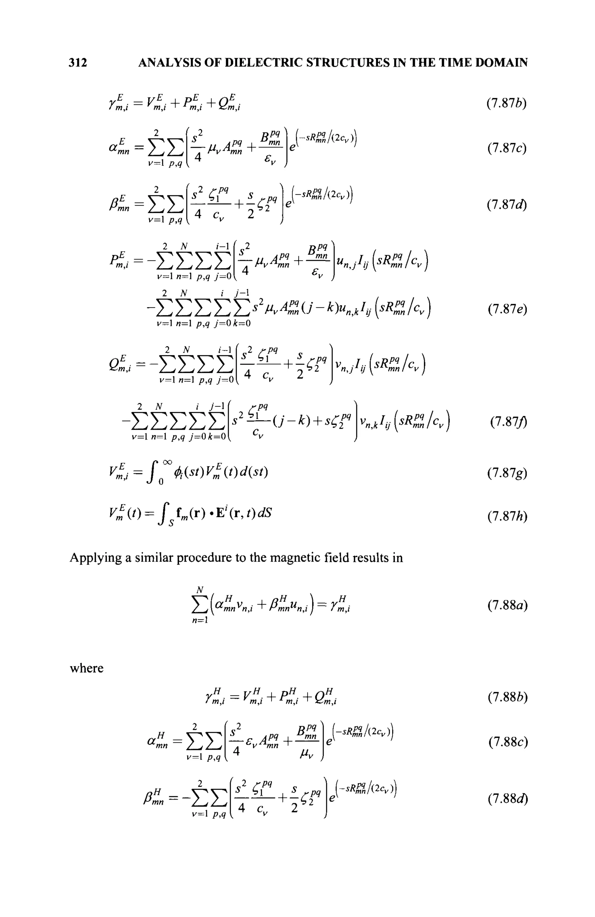
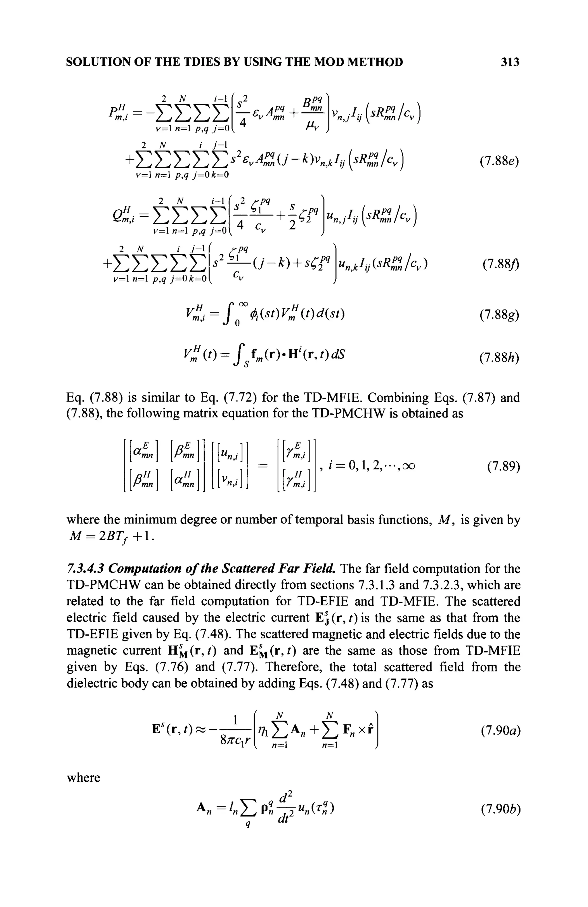
![314 ANALYSIS OF DIELECTRIC STRUCTURES IN THE TIME DOMAIN
F =/ Γ η ' — v (τ4
)
q M
(7.90c)
7
.
4 AN ALTERNATIVE MOD APPROACH
7.4.1 Alternate Solution to the TD-EFIE
In this section, an alternate MOD method is presented for solution of the TD-EFIE
without using the Hertz vector to represent the magnetic current. With this
modification, all terms related to the magnetic current in the MOD formulation for
TD-EFIE needs to be revised. In the spatial testing, the third term in Eq. (7.26),
which is related to the electric vector potential F(r,t) is rewritten. By substituting
the magnetic current expansion described in Eq. (7.2le) into this term, the
following result can be obtained based on Eq. (7.35) as:
fm (r),—VxFv (r,0>
N
Σ
я=1
Cm„,vMn(t) + ^2
р,ч
c„ dt ^(C)KfM„(C) (7.91)
In the temporal testing, similar to Eq. (7.38Й) and (7.40a), the time domain
magnetic current coefficient and its derivative can be expanded as
d °° ( 1 ^-1
;=o k=0
Φ№
(7.92)
(7.93)
Following a similar procedure as in section 7.3.1, and replacing Eqs. (7.35),
(7.386), and (7.40a) with Eqs. (7.91)-(7-93) results in a matrix equation
r0> ?(D
a--1 IÄ-.
(2)1 I «(2)
rmn
a,
К ] =
ym
у m,i
f/2)]
1/ m,i 1
(7.94)
where the elements related to the magnetic current are recomputed as](https://image.slidesharecdn.com/timeandfrequencydomainsolutionsofemproblemsusingintegralequationsandahybridmethodologyb-250205130750-568a5ba2/75/Time-and-Frequency-Domain-Solutions-of-EM-Problems-Using-Integral-Equations-and-a-Hybrid-Methodology-B-H-Jung-pdf-335-2048.jpg)
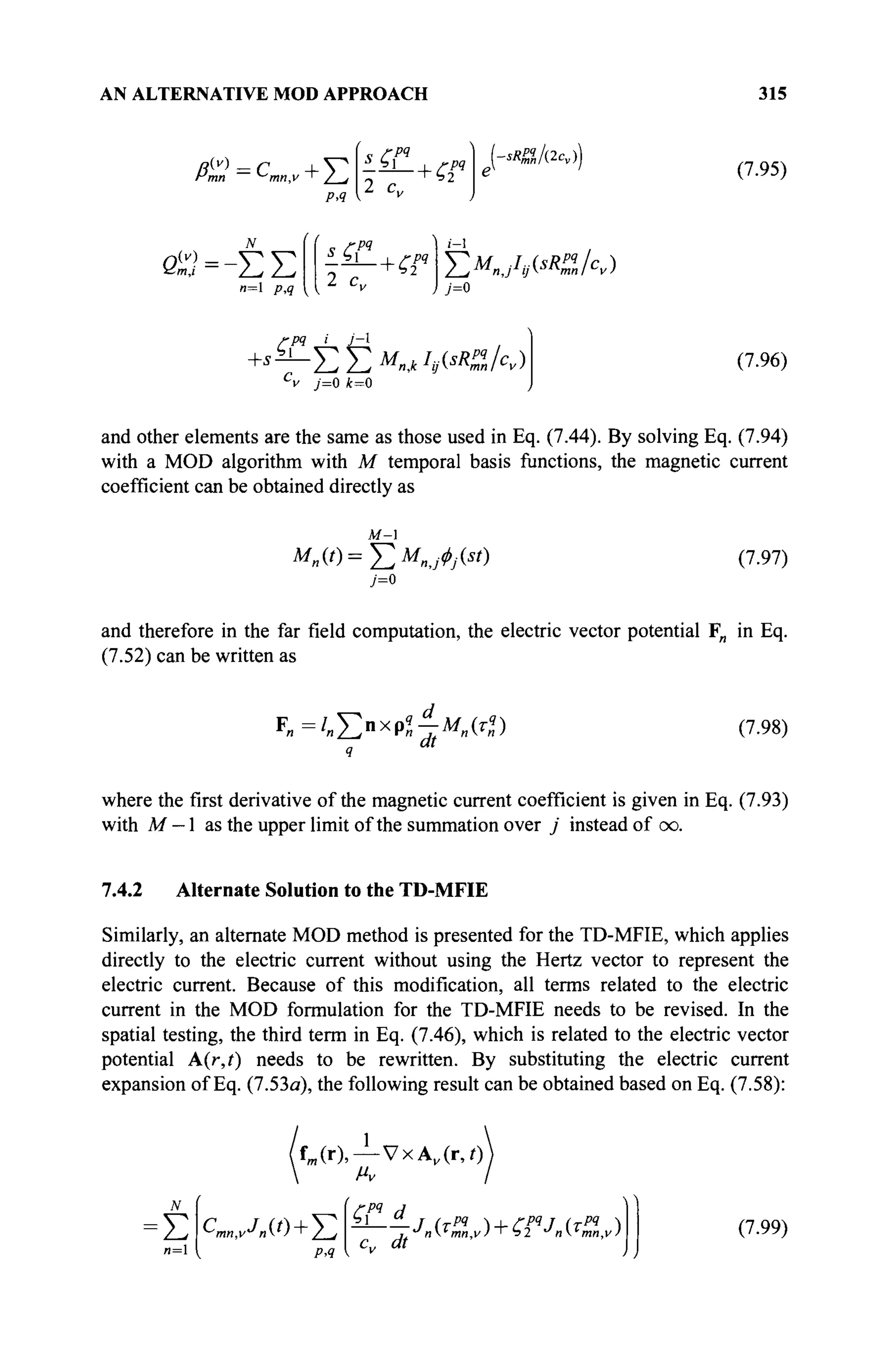
![NUMERICAL EXAMPLES 319
resonant frequencies of the structures. The transient electric and magnetic currents
on the dielectric surface and Θ- (or x-) components of the normalized far fields
along the backward direction is plotted. All solutions computed by the present
method are compared with the inverse discrete Fourier transform (IDFT) of the
frequency domain solutions of the FD-EFIE [15]. In addition, the far field for the
sphere is compared with the Mie series solution. Setting s = 109
and M = 80 is
sufficient to get accurate solutions. In all figures, a label with "(1)" and "(2)" mean
results computed by the formulation in section 7.3 and the alternative formulation
of section 7.4, respectively.
Figure 7.1. Triangle patching of three dielectric objects: (a) Sphere, (b) Cube, and (c)
Cylinder.](https://image.slidesharecdn.com/timeandfrequencydomainsolutionsofemproblemsusingintegralequationsandahybridmethodologyb-250205130750-568a5ba2/75/Time-and-Frequency-Domain-Solutions-of-EM-Problems-Using-Integral-Equations-and-a-Hybrid-Methodology-B-H-Jung-pdf-340-2048.jpg)
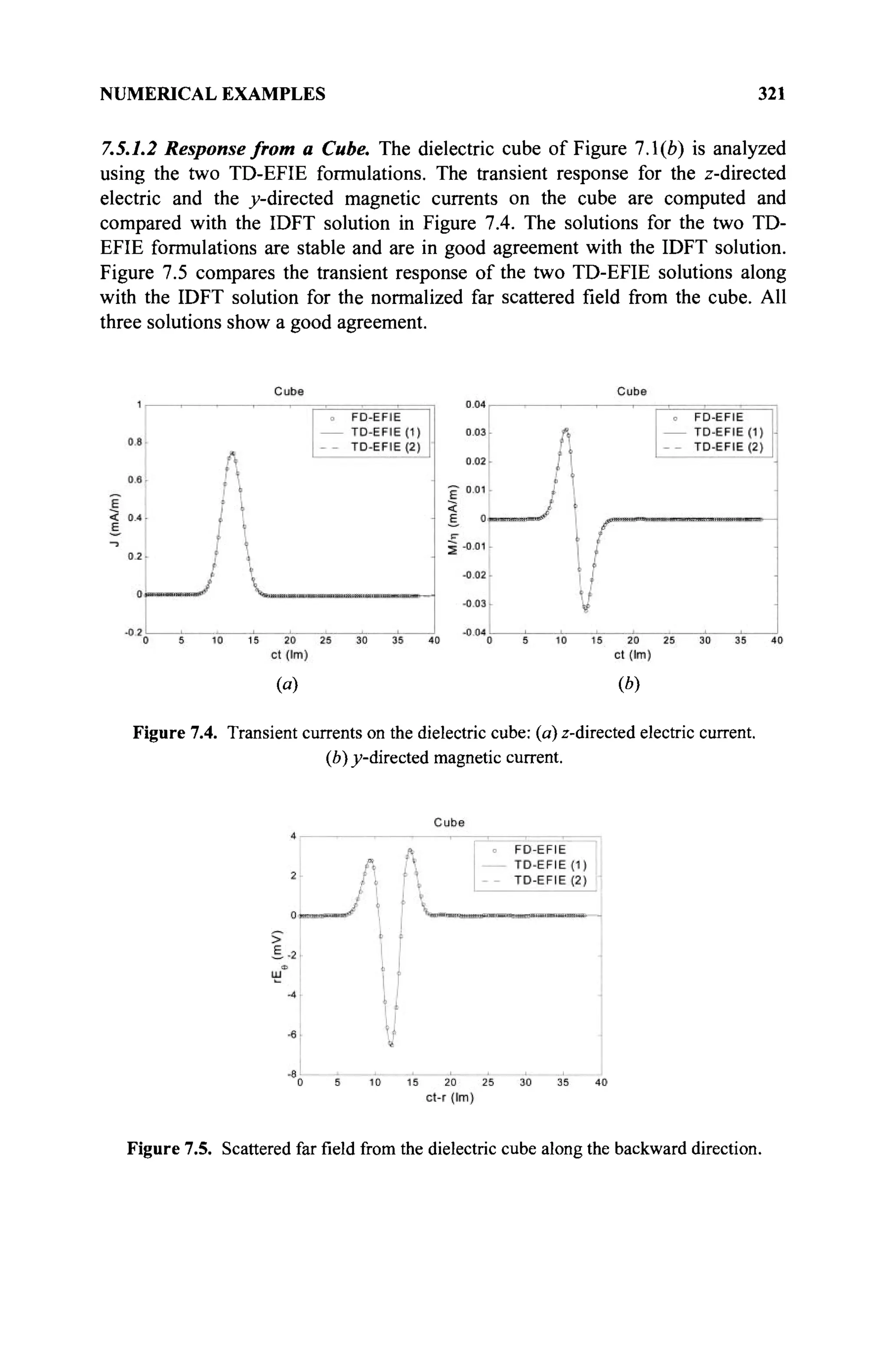
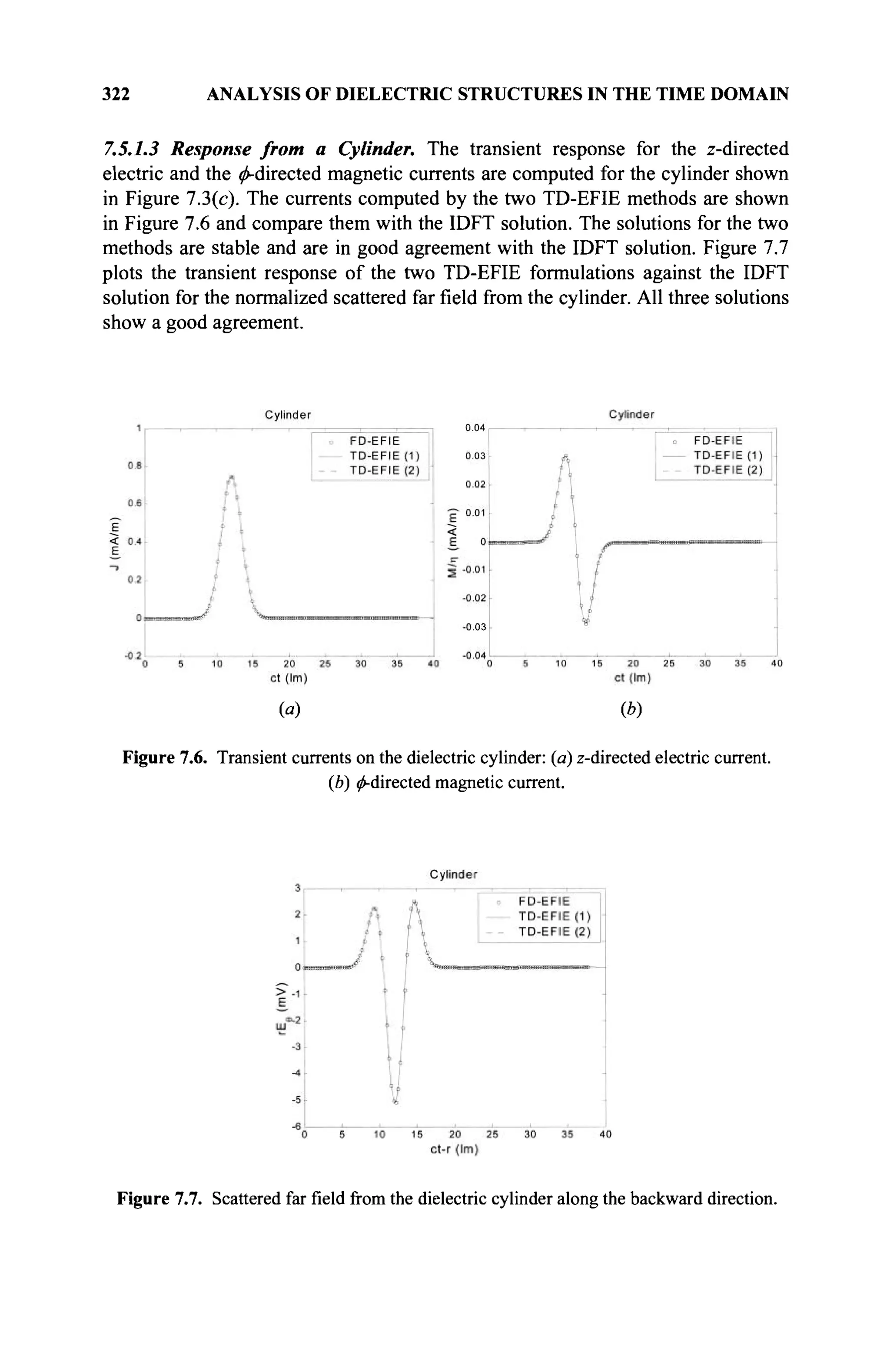
![NUMERICAL EXAMPLES 323
7.5.2 Using the TD-MFIE Formulations
In this section, the numerical results for three 3-D dielectric scatterers are
presented. They include a sphere and a cube as shown in Figure 7.1(a) and (b) and
a cone-cylinder shown in Figure 7.8. The three dielectric scatterers have a relative
permittivity er =2 and are placed in the free space. The results are computed
using the two TD-MFIE formulations of Eqs. (7.73) and (7.102). The surface of
the dielectric structures is modeled using planar triangular patches. The
discretizations for the dielectric sphere and the cube are the same as stated in
section 7.5.1. The dielectric cone-cylinder has a radius of 0.5 m, a height of 0.5 m
for both the cone and the cylinder. It has a total of 576 patches with 864 edges.
Figure 7.8. Triangle patching of a cone-cylinder.
All scatterers are illuminated by a Gaussian plane wave in which the
magnetic field is given by
1 - 4 ^ 2 4
H'(r,i) = - k x E 0 - = ^ g r
and χ = —(ct-ct0-r-k) (7.116)
η 4πΤ Τ
where к is the unit vector along the direction of the wave propagation. T is the
pulse width of the Gaussian impulse, and t0 is a time delay that represents the
time at which the pulse peaks at the origin. The field is incident from ф = 0° and
θ = 0° with к = —z , so that E0 = x. In the numerical computation, T = 8 lm
and ctQ =12 lm is used. This bandwidth of the pulse is then 125 MHz, so it does
not include any internal resonant frequencies of the structures. The numerical
results to be shown are the transient electric and magnetic currents on the
dielectric surface, Θ- (or x-) components of the normalized far field in the
backward direction, and the radar cross section (RCS). All solutions computed by
the TD-MFIE formulations are compared with the IDFT of the frequency domain
solutions given by the frequency domain magnetic field integral equation (FD-
MFIE) [15]. In addition, the far field solution for the sphere is compared with the
Mie series solution. Setting s = 109
and M = 80 is sufficient to obtain accurate](https://image.slidesharecdn.com/timeandfrequencydomainsolutionsofemproblemsusingintegralequationsandahybridmethodologyb-250205130750-568a5ba2/75/Time-and-Frequency-Domain-Solutions-of-EM-Problems-Using-Integral-Equations-and-a-Hybrid-Methodology-B-H-Jung-pdf-344-2048.jpg)
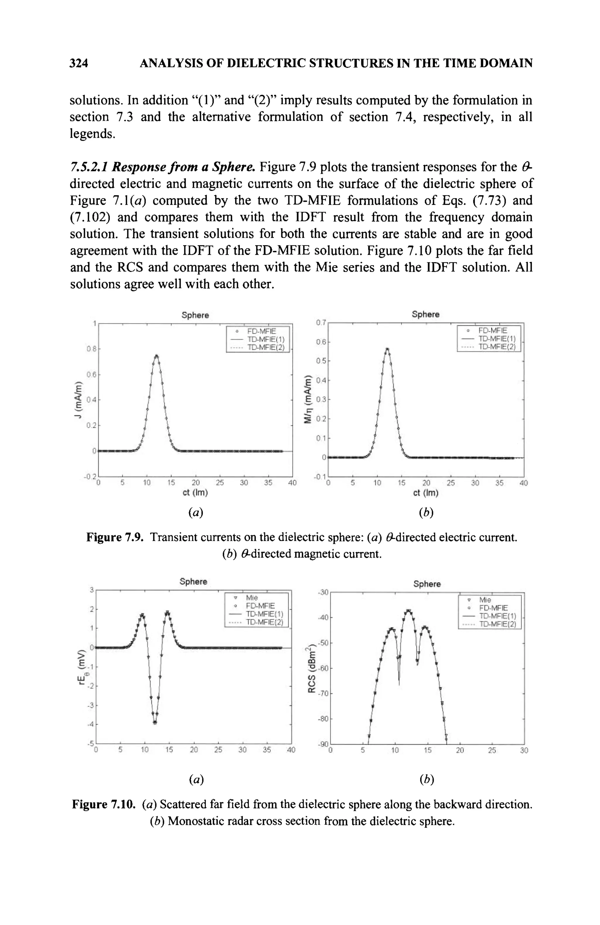
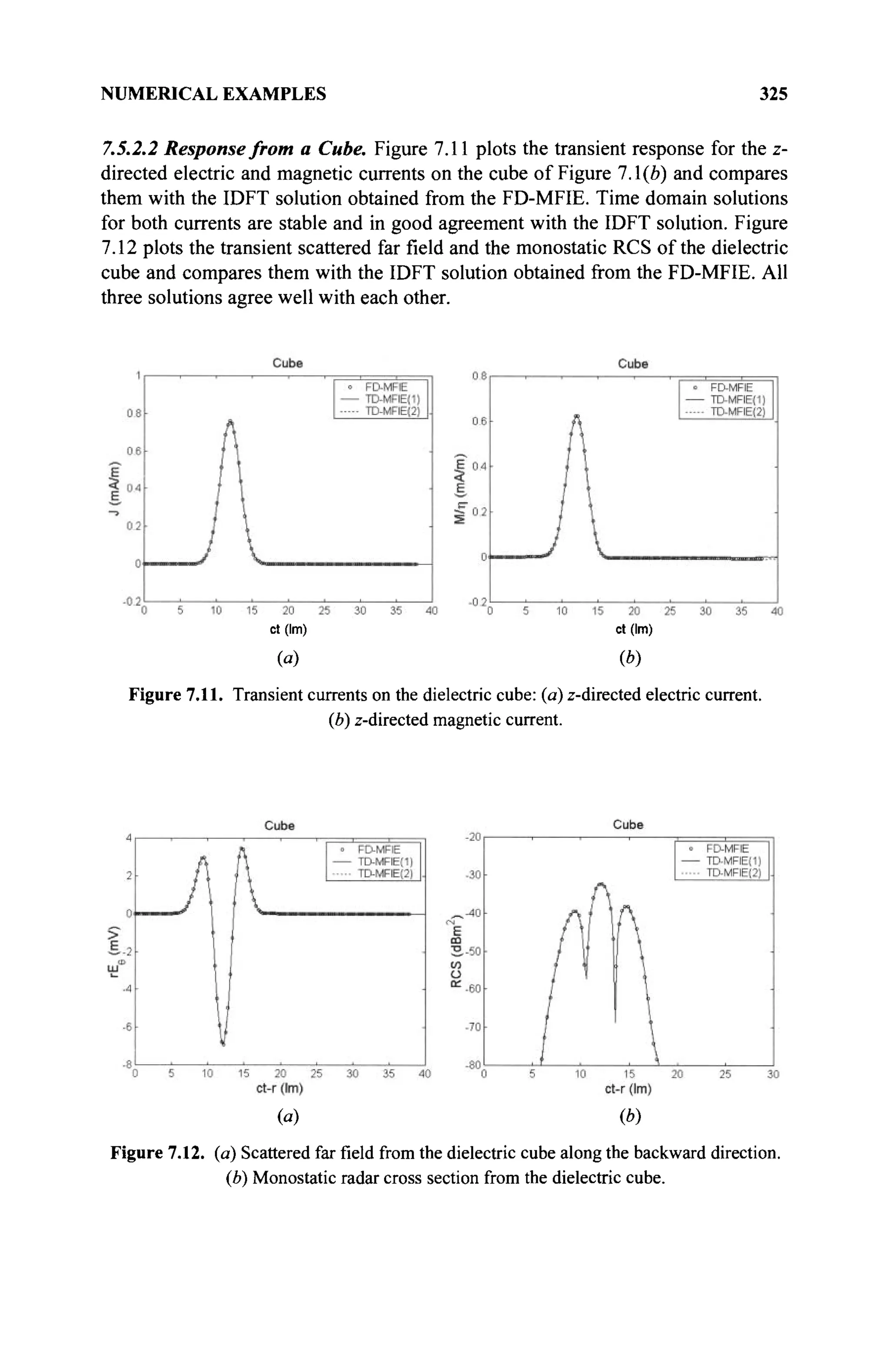
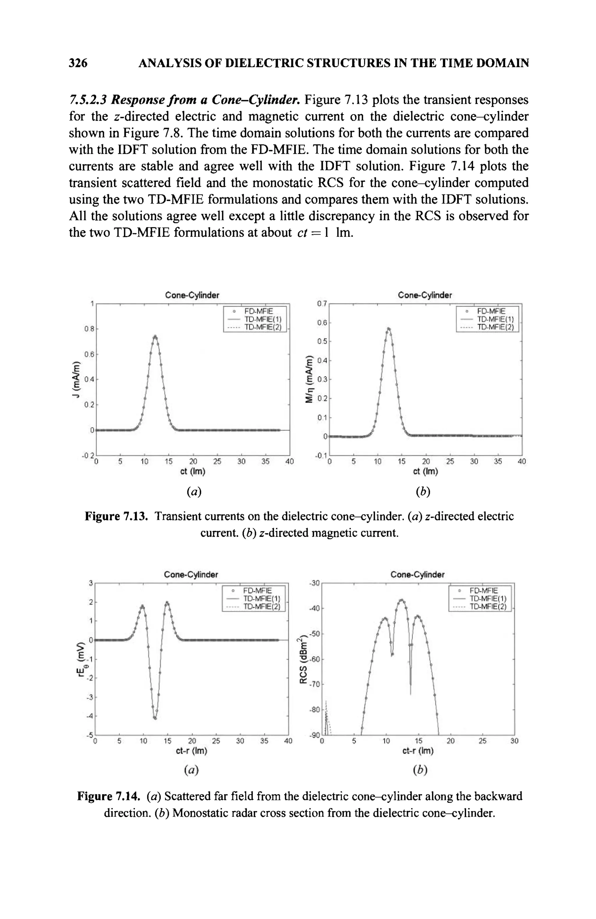
![NUMERICAL EXAMPLES 327
7.5.3 Using the TD-PMCHW Formulations
In this section, the numerical results for various 3-D dielectric scatterers are
presented using the two TD-PMCHW formulations given by Eqs. (7.89) and
(7.110). All scatterers have a relative permittivity £r=2 and are placed in free
space. They are illuminated by a Gaussian plane wave defined by Eqs. (7.115) and
(7.116). The field is incident from φ = 0° and # = 0° with к = —z, and E0 = x.
A pulse width of T = 2 lm and a delay of ct0 = 4 lm are chosen for the
numerical computation. This pulse has a bandwidth of 500 MHz, which include
several internal resonant frequencies of the structures to be analyze'd. Setting
5 = 2xl09
and M = 80 is sufficient to get accurate solutions. All solutions are
computed using the TD-PMCHW, and the results are compared with the IDFT of
the frequency domain solutions obtained by the PMCHW formulation [15]. The
frequency domain solution is generated in the range of 0+
-500 MHz with 128
samples. The far field is Θ- (or x-) component of the electric field and are
computed along the backward direction ( +z axis) of the scatterers. The figure
legends, "(I)" and "(II)" imply that the results are computed using the PMCHW
formulation described in section 7.3 and the alternative formulation of section 7.4,
respectively.
First, consider a dielectric sphere as shown in Figure 7.1(a) using the
same number of patches and edges used for generating the results of sections 7.5.1
and 7.5.2. Figure 7.15 plots the transient response for the ^-directed electric and
magnetic currents on the sphere at Θ = 90° and are computed using the two TD-
PMCHW formulations and compared with the IDFT results using the FD-
PMCHW solutions. The locations and the directions of the currents on the
structure are depicted in the insets of the figures. It can be found that the solutions
from the TD-PMCHW formulations are stable and are in good agreement with the
IDFT solutions.
(«) (b)
Figure 7.15. Transient currents on the dielectric sphere at Θ = 90°: (a) Electric current at
ф = 7.5°. (b) Magnetic current at ф = 172.5°.](https://image.slidesharecdn.com/timeandfrequencydomainsolutionsofemproblemsusingintegralequationsandahybridmethodologyb-250205130750-568a5ba2/75/Time-and-Frequency-Domain-Solutions-of-EM-Problems-Using-Integral-Equations-and-a-Hybrid-Methodology-B-H-Jung-pdf-348-2048.jpg)

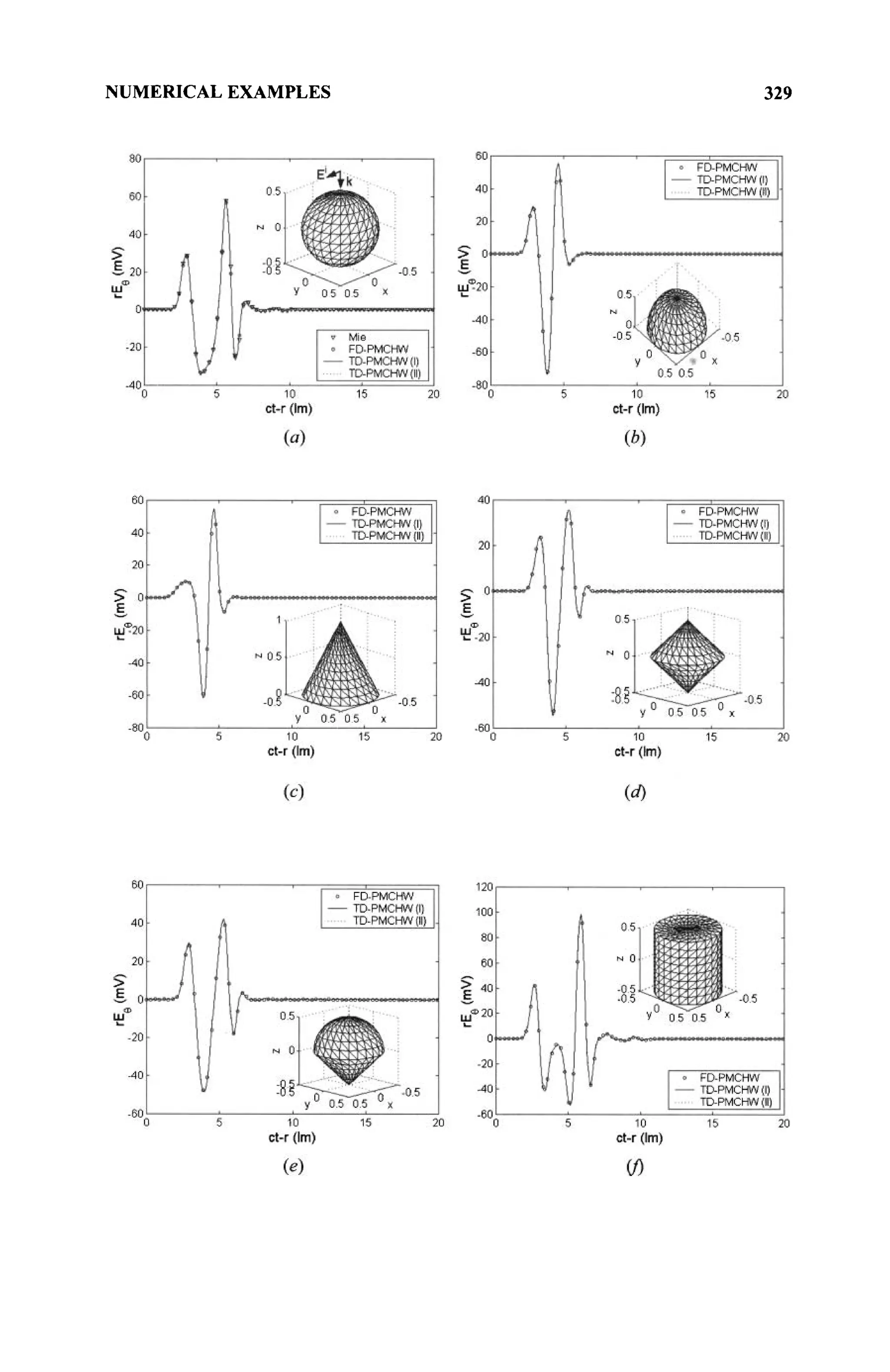
![330 ANALYSIS OF DIELECTRIC STRUCTURES IN THE TIME DOMAIN
(g) (h)
Figure 7.16. Backward scatteredfieldalong the +z direction from the dielectric
structures: (a) Sphere, (b) Hemisphere, (c) Cone, (d) Double cones, (e) Hemisphere-cone
(/) Cylinder, (g) Hemisphere-cylinder, (h) Cone-cylinder.
7.5.4 Using the TD-CFIE Formulation
The numerical results for 3-D dielectric scatterers computed using the TD-CFIE
formulation given by Eq. (7.85) now are presented. The scatterers are illuminated
by a Gaussian plane wave defined by Eq. (7.115) and (7.116). The field is incident
from φ = 0° and θ = 0° with к = —г, and E0 = x. A pulse width of T = 4 lm
and a time delay ct0 = 6 lm is chosen for the numerical computation. Setting
s = 0.9xl09
and M = 40 is sufficient to get accurate solutions. All solutions
computed by the TD-CFIE formulation are compared with the IDFT of the FD-
CFIE solutions [15] in the bandwidth of 0+
-500 MHz with 128 samples. All
dielectric structures have a relative permittivity εr = 2 and are placed in free
space. The shaded patches on the structure shown in the inset of the figures
indicate the location of the current to be observed associated with the common
edge. The far field solutions are Θ- (or x-) components of the electric field
computed along the backward direction ( +z axis) from the scatterers. The
following two combinations of the spatial testing functions for the TD-CFIE are
considered [15]:
(tm + gm, EFIE) + (-fm + gm, MFIE) or
(fm-gm,EFIE) + (fm+gm,MFIE)
A general form of the testing can be represented by involving the coefficients fE,
gE, fH, and fH, which can be set as either + 1 or — 1.
fE {fm, EFIE) + gE (gm, EFIE) + fH (fm, MFIE) + gH {gm, MFIE)](https://image.slidesharecdn.com/timeandfrequencydomainsolutionsofemproblemsusingintegralequationsandahybridmethodologyb-250205130750-568a5ba2/75/Time-and-Frequency-Domain-Solutions-of-EM-Problems-Using-Integral-Equations-and-a-Hybrid-Methodology-B-H-Jung-pdf-351-2048.jpg)
![NUMERICAL EXAMPLES 331
Similar to the FD-CFIE formulation introduced in Chapter 3 [15], it is possible to
drop one of the testing terms to generate 16 different formulations (i.e., setting one
of the coefficients to zero with the coefficients that can be either+1 or —1 [14]).
These formulations include TENE-TH for gH = 0, TENE-NH for fH = 0, TE-
THNH for gE = 0, and NE-THNH for fE = 0. However, for TD-CFIE, none of
the 16 formulations provides valid transient solutions. In this section, numerical
results using only the testing coefficients fE =1, gE = 1, fH = — 1, and gH = 1
and the combination parameter of к = 0.5 are presented.
7.5.4.1 Response from a Sphere. Consider the dielectric sphere shown in'Figure
7.1(a). Figure 7.17 plots the transient response of the ^-directed electric current
density at the shaded patch on the sphere (Θ = 90° and ф = 7.5°) computed by the
TD-CFIE formulation and it is compared with the IDFT of the frequency domain
solutions. In Figure 7.17, it is found that the solutions computed using the MOD
method using the TD-CFIE are stable and agree well with the IDFT solution.
Figure 7.18 depicts the transient response for the backward scattered far field
obtained by the TD-CFIE formulation along with the Mie series solution and the
IDFT solution. All three solutions show very good agreement.
7.5.4.2 Response from a Hemisphere—Cone and a Double Cone. The next
example deals with a hemisphere terminated by a cone. The radius of the
hemisphere is 0.5 m and the height of the cone along the z-direction is 0.5 m. This
structure is divided into 480 triangular patches with a total number of 720 edges.
Figure 7.19 plots the transient response for the ^-directed electric and magnetic
currents at the shaded patch on the sphere (Θ = Ί5° and φ = 7.5°) computed by
the TD-CFIE formulation and compares with the IDFT solution. In Figure 7.19, it
is shown that the solutions obtained by the MOD method along with the TD-CFIE
are stable and agree well with the IDFT solution. Figure 7.20 presents the transient
response for the backward scattered far field from the dielectric hemisphere-cone
obtained by the TD-CFIE along with the IDFT of the FD-CFIE solution. Two
solutions agree well as is evident from the figure.
Finally, a double cone dielectric structure is considered, which is shown
in Figure 7.21. The height of the cones along the z-direction is 1 m and the radius
at z = 0 is 0.5 m. This structure is divided into 432 triangular patches with a total
of 648 edges. In this figure, the backward scattered field computed using the TD-
CFIE formulation is compared with the IDFT of the frequency domain result. The
agreement of the solution computed using the TD-CFIE and the IDFT of the FD-
CFIE solution is excellent.](https://image.slidesharecdn.com/timeandfrequencydomainsolutionsofemproblemsusingintegralequationsandahybridmethodologyb-250205130750-568a5ba2/75/Time-and-Frequency-Domain-Solutions-of-EM-Problems-Using-Integral-Equations-and-a-Hybrid-Methodology-B-H-Jung-pdf-352-2048.jpg)
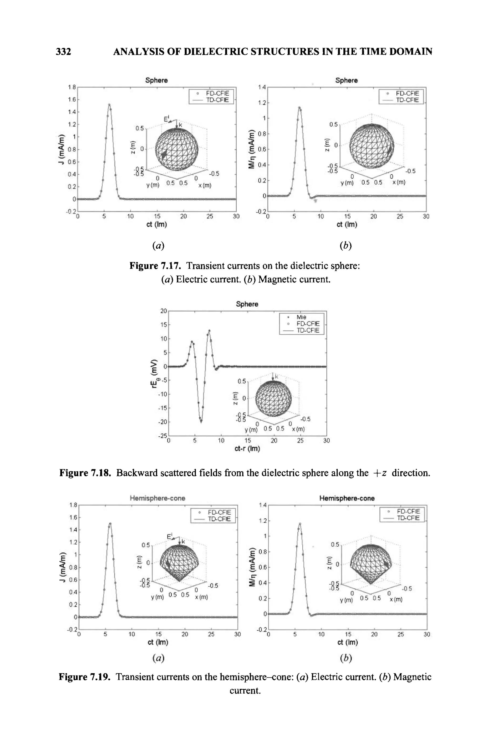
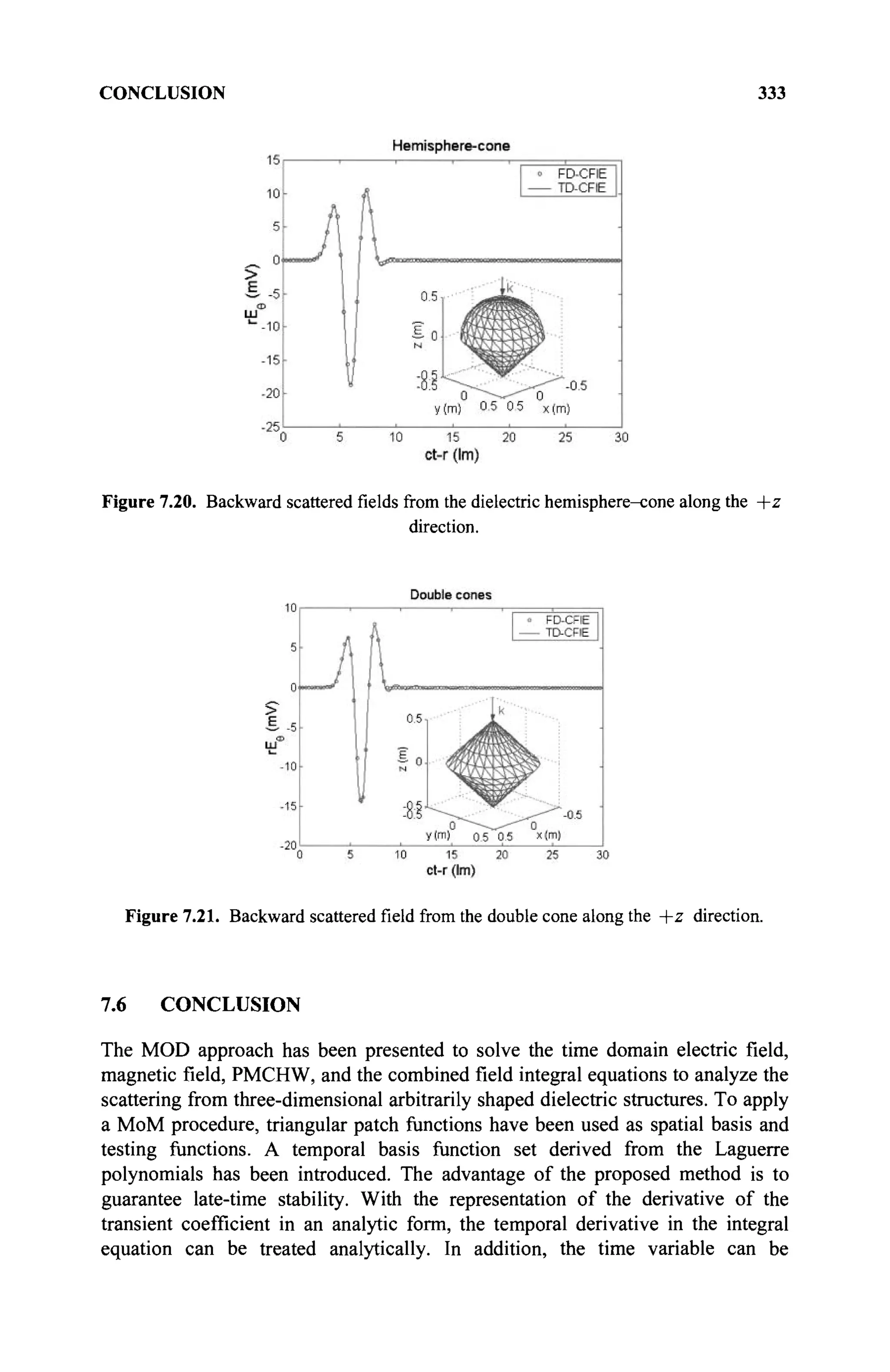
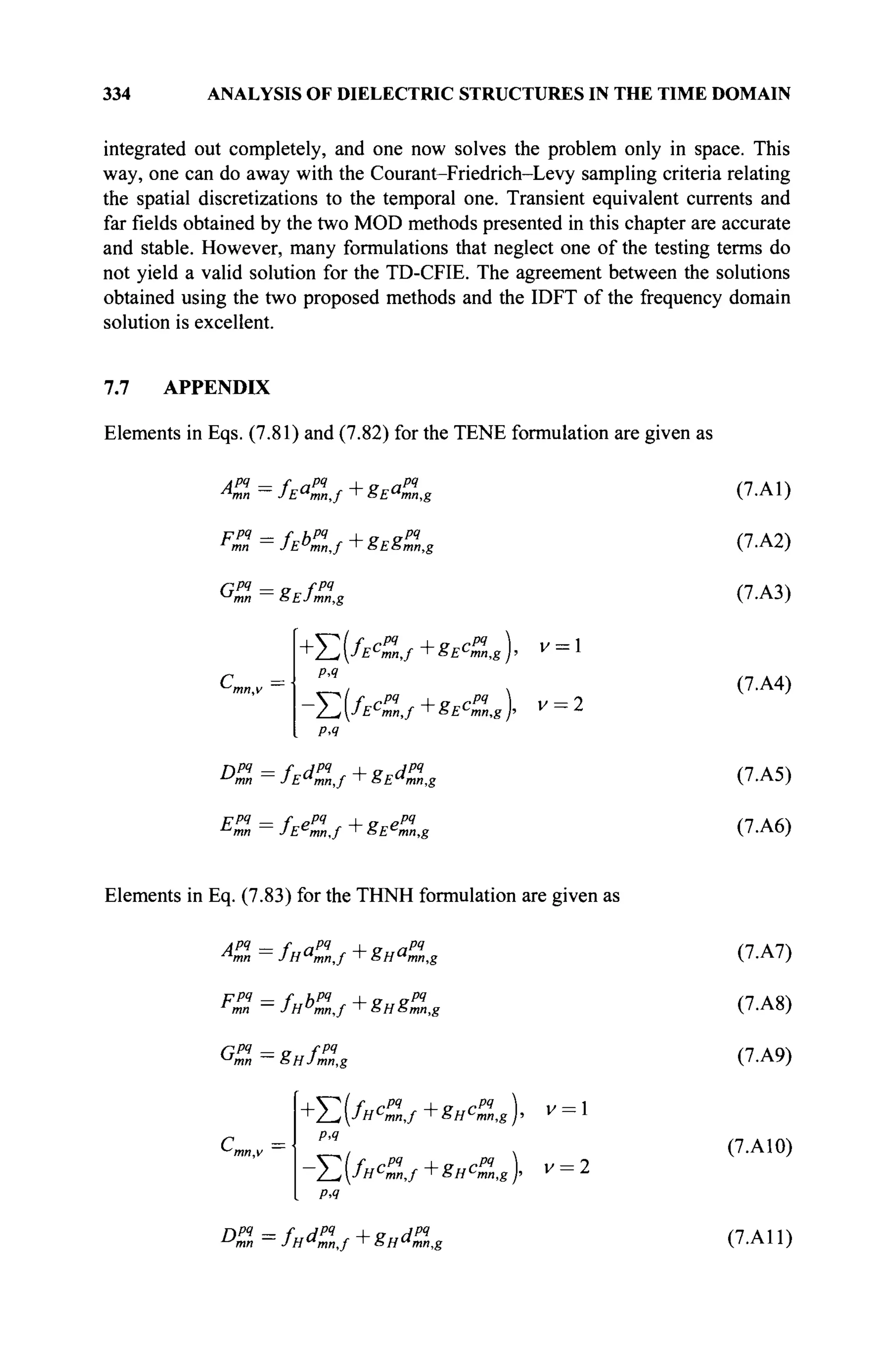
![APPENDIX 335
ppq — f ppq , „ ppq
mn,g (7.A12)
And the integrals in Eq. (7.A1)-(7.A12) are given by
/^=^/sg^(r)./5V'.f^(r')f^
cP
mlg=jsëP
m(r>nx^(r)dS
epq
, :
mn,j
mn,g
(7.A13)
(7.A14)
(7.A15)
(7.A16)
(7.A17)
(7.A18)
(7.A19)
(7.A20)
(7.A21)
(7.A22)
(7.A23)
where R is a unit vector along the direction r —r'. The evaluations of Eqs.
(7.A13)-(7.A23) have been presented in [24-30]. The integral associated with the
incident fields are expressed as
V?v
t)-
Js fEfm (r) + g£gm (r) · E' (r, t)dS, v = 1
0, v = 2
(7.A24)
rH(v)
(0-
fsfHW + BHim(W(r, t)dS, v = 1
0, v = 2
(7.A25)](https://image.slidesharecdn.com/timeandfrequencydomainsolutionsofemproblemsusingintegralequationsandahybridmethodologyb-250205130750-568a5ba2/75/Time-and-Frequency-Domain-Solutions-of-EM-Problems-Using-Integral-Equations-and-a-Hybrid-Methodology-B-H-Jung-pdf-356-2048.jpg)
![336 ANALYSIS OF DIELECTRIC STRUCTURES IN THE TIME DOMAIN
REFERENCES
[I] S. M. Rao, Time Domain Electromagnetics, Academic Press, New York, 1999.
[2] H. Mieras and С L. Bennet, "Space-time integral equation approach to dielectric
targets," IEEE Trans. Antennas Prop., Vol. 30, pp. 2-9, 1982.
[3] D. A. Vechinski, S. M. Rao, and T. K. Sarkar, "Transient scattering from three-
dimensional arbitrary shaped dielectric bodies," J. Opt. Soc. Amer., Vol. 11, pp.
1458-1470, 1994.
[4] B. P. Rynne, "Time domain scattering from dielectric bodies," Electromagnetics,
Vol. 14, pp. 181-193,1994.
[5] E. Marx, "Integral equation for scattering by a dieleotric," IEEE Trans. Antennas
Prop., Vol. 32, pp. 166-172, 1984.
[6] M. D. Pocock, M. J. Bluck and S. P. Walker, "Electromagnetic scattering from 3-
D curved dielectric bodies using time domain integral equations," IEEE Trans.
Antennas Prop., Vol. 46, pp. 1212-1219, 1998.
[7] N. T. Gres, A. A. Ergin, E. Michielssen and B. Shanker, "Volume-integral-
equation based analysis of transient electromagnetic scattering from three-
dimensional inhomogeneous dielectric objects," Radio Sei., Vol. 36, pp. 379-386,
2001.
[8] T. K. Sarkar, W. Lee, and S. M. Rao, "Analysis of transient scattering from
composite arbitrarily shaped complex structures," IEEE Trans. Antennas Prop.,
Vol. 48, pp. 1625-1634, 2000.
[9] S. M. Rao and T. K. Sarkar, "Implicit Solution of time-domain integral equations
for arbitrarily shaped dielectric bodies," Microw. Opt. Tech. Lett, Vol. 21, pp.
201-205, 1999.
[10] B. H. Jung and T. K. Sarkar, "Time-domain electric-field integral equation with
central finite difference," Microw. Opt. Tech. Lett, Vol. 31, pp. 429-435, 2001.
[II] T. K. Sarkar and J. Koh, "Generation of a wide-band electromagnetic response
through a Laguerre expansion using early-time and low-frequency data," IEEE
Trans. Microwave Theory Tech., Vol. 50, pp. 1408-1416, 2002.
[12] B. H. Jung, T. K. Sarkar, Y.-S. Chung, Z. Ji, and M. Salazar-Palma, "Analysis of
transient electromagnetic scattering from dielectric objects using a combined-field
integral equation," Microw. Opt. Tech. Lett, Vol. 40, pp. 476^481, 2004.
[13] B. H. Jung, Y.-S. Chung, and T. K. Sarkar, "Time-domain EFIE, MFIE, and CFIE
formulations using Laguerre polynomials as temporal basis functions for the
analysis of transient scattering from arbitrary shaped conducting structures," J.
Electromagn. Waves Appl., Vol. 17. pp. 737-739, 2003.
[14] X. Q. Sheng, J. M. Jin, J. M. Song, W. С Chew, and С. С. Lu, "Solution of
combined-field integral equation using multilevel fast multipole algorithm for
scattering by homogeneous bodies," IEEE Trans. Antennas Prop., Vol. 46, pp.
1718-1726, 1998.
[15] B. H. Jung, T. K. Sarkar, and Y.-S. Chung, "A survey of various frequency
domain integral equations for the analysis of scattering from three-dimensional
dielectric objects," J. Electromagn. Waves Appl., Vol. 16. pp. 1419-1421, 2002.
[16] S. M. Rao, D. R. Wilton, and A. W. Glisson, "Electromagnetic scattering by
surfaces of arbitrary shape," IEEE Trans. Antennas Prop., Vol. 30, pp. 409-418,
1982.
[17] T. K. Sarkar, S. M. Rao, and A. R. Djordjevic, "Electromagnetic Scattering and
Radiation from Finite Microstrip Structures," IEEE Transactions on Microwave
Theory and Techniques, Vol. 38, No. 11, pp. 1568-1575, Nov. 1990.
[18] S. M. Rao and D. R. Wilton, "£-field, Я-field, and combined field solution for
arbitrarily shaped three-dimensional dielectric bodies," Electromagnetics, Vol.
10, pp. 407^121, 1990.](https://image.slidesharecdn.com/timeandfrequencydomainsolutionsofemproblemsusingintegralequationsandahybridmethodologyb-250205130750-568a5ba2/75/Time-and-Frequency-Domain-Solutions-of-EM-Problems-Using-Integral-Equations-and-a-Hybrid-Methodology-B-H-Jung-pdf-357-2048.jpg)
![REFERENCES 337
[19] S. M. Rao, Electromagnetic Scattering and Radiation of Arbitrarily-Shaped
Surfaces by Triangular Patch Modeling, PhD Dissertation, University of
Mississippi, Miss. 1980.
[20] L. Debnath, Integral Transforms and Their Applications, CRC Press, Boca Raton,
FL., 1995.
[21] A. D. Poularikas, The Transforms and Applications Handbook, IEEE Press, New
York, 1996.
[22] I. S. Gradshteyn and I. M. Ryzhik, Table of Integrals, Series, and
Products, Academic Press, New York, 1980.
[23] J. Van Bladel, Electromagnetic Fields, Hemisphere Publishing Corporation, New
York, 1985.
[24] D. R. Wilton, S. M. Rao, A. W. Glisson, D. H. Schaubert, О. M. Al-Bundak, and
С. M. Butler, "Potential integrals for uniform and linear source distributions on
polygonal and polyhedral domains," IEEE Trans. Antennas Prop., Vol. 32, pp.
276-281, 1984.
[25] R. D. Graglia, "Static and dynamic potential integrals for linearly varying source
distributions in two- and three-dimensional problems," IEEE Trans. Antennas
Prop., Vol. 35, pp. 662-669, 1987.
[26] S. Caorsi, D. Moreno, and F. Sidoti, "Theoretical and numerical treatment of
surface integrals involving the free-space Green's function," IEEE Trans.
Antennas Prop., Vol. 41, pp. 1296-1301, 1993.
[27] R. D. Graglia, "On the numerical integration of the linear shape functions times
the 3-D Green's function or its gradient on a plane triangle," IEEE Trans.
Antennas Prop., Vol. 41, pp. 1448-1455, 1993.
[28] T. F. Eibert and V. Hansen, "On the Calculation of potential integrals for linear
source distributions on triangular domains," IEEE Trans. Antennas Prop., Vol.
43, pp. 1499-1502, 1995.
[29] R. E. Hodges and Y. Rahmat-Samii, "The evaluation of MFIE integrals with the
use of vector triangle basis functions," Microw. Opt. Tech. Lett., Vol. 14, pp. 9-
14, 1997.
[30] P. Yla-Oijala and M. Taskinen, "Calculation of CFIE impedance matrix elements
with RWG and nx RWG functions," IEEE Trans. Antennas Prop., Vol. 51, pp.
1837-1846,2003.](https://image.slidesharecdn.com/timeandfrequencydomainsolutionsofemproblemsusingintegralequationsandahybridmethodologyb-250205130750-568a5ba2/75/Time-and-Frequency-Domain-Solutions-of-EM-Problems-Using-Integral-Equations-and-a-Hybrid-Methodology-B-H-Jung-pdf-358-2048.jpg)
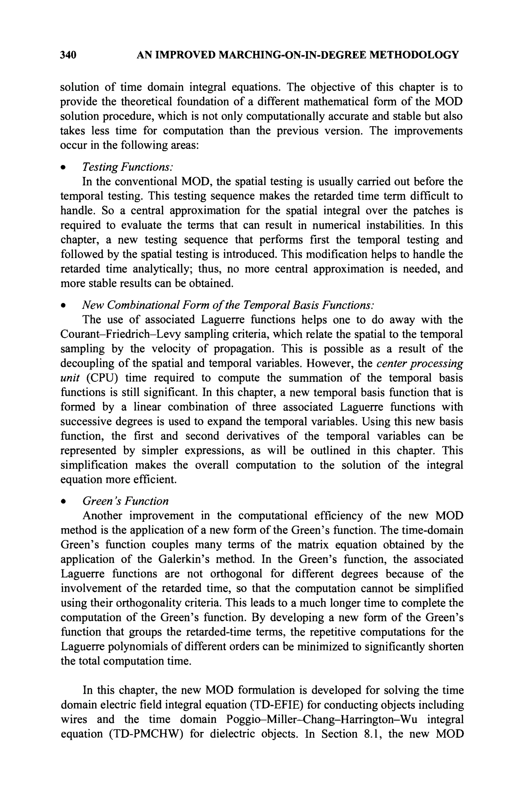
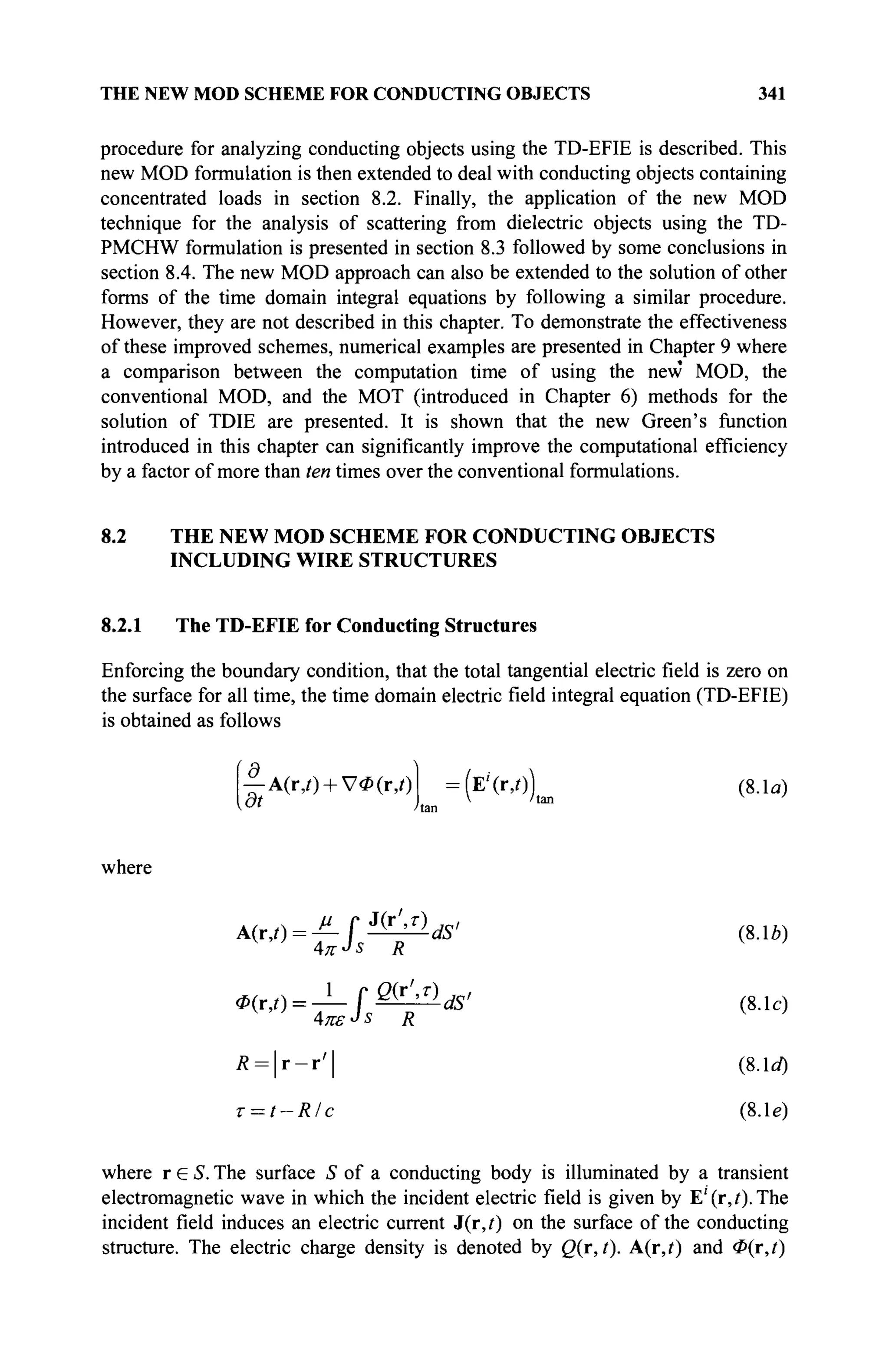
![342 AN IMPROVED MARCHING-ON-IN-DEGREE METHODOLOGY
represent the magnetic vector and electric scalar potentials, respectively. The
symbol R represents the distance between the observation point r and the source
point r'. τ is the retarded time resulting from the delay for the transmission of the
field from the source point to the field point, μ and ε are the permeability and
the permittivity of the medium, and с is the velocity of the propagation of the
electromagnetic wave in that space. The subscript "tan" denotes the tangential
components. Note that the integrals over the surface S in Eqs. (8.1Л) and (8.1c)
are transformed into line integrals over the wire length L when the scatterer is a
conducting wire.
To simplify the time integral in the TD-EFIE analytically, the Hertz
vector u(r, t) is introduced in the MOD method and it is defined as [1]
J(r,0 = —n(r,/) (8.2)
at
and the relation between the Hertz vector and the electric charge density Q(r, t) is
given by
g(r,0 = - V - u ( r , 0 (8.3)
Substituting Eqs. (8.2) and (8.3) into Eq. (8.1), the TD-EFIE can be expressed in
terms of the Hertz vector as
=ИГ
'С (8
·4
)
v 'tan
8.2.2 Expansion Functions in Space and Time
The Hertz vector in Eq. (8.4) is now expanded using the RWG vector functions,
which have been introduced in Eq. (6.13) of Section 6.3, as the spatial basis
functions. This result in
N
u(r,0 = ^>„(0f„(r) (8.5)
и=1
Note that in Eq. (8.5), the spatial and temporal variables are separated. It is
important to note that the spatial basis functions do not need to be limited by the
choice of the RWG vector functions [2,3]. In fact, it is possible to choose instead
the higher-order basis functions [4] or of some other type.
In the conventional MOD method introduced in Chapters 5-7, the
temporal basis functions chosen are the associated Laguerre functions
<f>j(st), which have been described by Eq. (6.72) in section 6.5. Mathematically,
they are written as
AKdt2J
s R AnsJs R](https://image.slidesharecdn.com/timeandfrequencydomainsolutionsofemproblemsusingintegralequationsandahybridmethodologyb-250205130750-568a5ba2/75/Time-and-Frequency-Domain-Solutions-of-EM-Problems-Using-Integral-Equations-and-a-Hybrid-Methodology-B-H-Jung-pdf-362-2048.jpg)
![THE NEW MOD SCHEME FOR CONDUCTING OBJECTS 343
4>j{st) -
e-s
"2
L,(st) / > 0
yV
' - (8.6)
0 ? < 0
where £ (t) is the Laguerre polynomial of degree j and 5 is a scaling factor.
The associated Laguerre function is causal (i.e., defined over the domain
[0,+oo))and convergent to zero as time goes to infinity [5,6]. To improve the
computational efficiency, the temporal basis function is represented by a
combination of three associated Laguerre functions with successive degrees
multiplied by some unknown constants for the transient coefficient un (t) as [7]
00
«η(0 = Σ ип,Д^(*О-2^+1(*О + 0у+2(*О) (8.7)
j=0
Referring to the property of the Laguerre polynomials presented in the appendix of
Chapter 5, the derivative of the Laguerre polynomials can be expressed as a sum
of its lower-order components as
^Lj(st) = -L%(st) = -f^Lpist) (8.8)
"' p=0
From Eq. (8.8), the derivative of the associated Laguerre function is written as
d s J
~l
—éj (st) = --<t>j (st) -sY,(l>p (st) (8.9)
Using the property given by Eq. (8.9), the first and second derivatives of the
transient coefficient un(t) of Eq. (8.7) can be derived and represented as a
combination of associated Laguerre functions of different degrees by the
following:
-rMO = Σ 7 « 4 , ( ^ ( Î / ) - ^ + 2 ( J 0 ) (8.10α)
"' j=o l
rP" oo ç 2
at J=0 4
In contrast to the conventional MOD method [2, 3] in which the transient
variable is expanded by a single associated Laguerre function set </>Asi) as
depicted by Eq. (6.73), the new temporal basis function presented here is formed
by a combination of three associated Laguerre functions, ^y(.sO> $j+(^t), and
φ,+2 (si
), f°r e a c n
degree j . By using this combinational temporal basis function](https://image.slidesharecdn.com/timeandfrequencydomainsolutionsofemproblemsusingintegralequationsandahybridmethodologyb-250205130750-568a5ba2/75/Time-and-Frequency-Domain-Solutions-of-EM-Problems-Using-Integral-Equations-and-a-Hybrid-Methodology-B-H-Jung-pdf-363-2048.jpg)
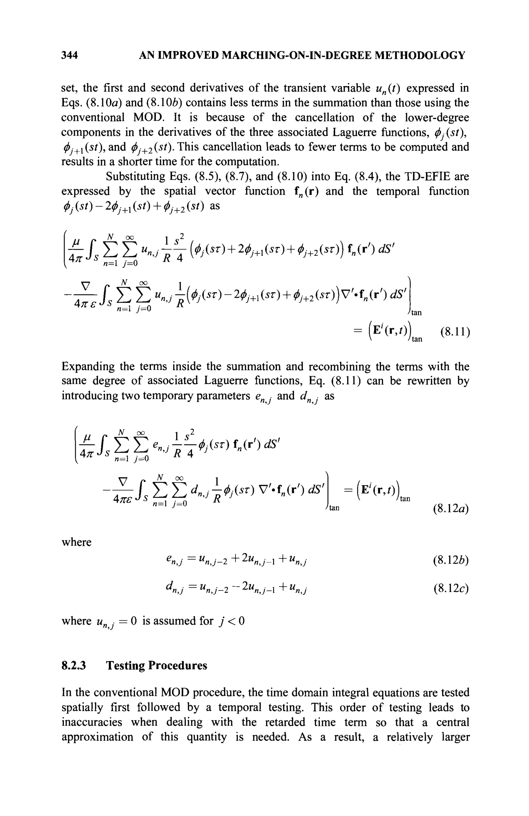
![THE NEW MOD SCHEME FOR CONDUCTING OBJECTS 345
approximation error is induced. To overcome this problem, the testing sequence is
revised to have the temporal testing before the spatial one. Also, through this
procedure, the time variable can be completely eliminated from the final
computations. Applying the temporal testing with a testing function φί (st) yields
Απ
N oo
Jl Σ Σ ^ΐΊ,τΠ, №Mj&)d(st)f„(r')ds!
~IS t £ > i C *<">w<*>v
'-f
«^ds
'
/ ^(i/)E'(r,/)rf(iO
*J 0
(8.13)
It is important to note that the basis functions contain a combination of three
associated Laguerre functions, whereas only one is used for testing.
Based on the integral property of the associated Laguerre functions given
in the appendix of Chapter 5, the integrals in I^^sR/c) can be evaluated as
J
»oo
φί(8ί)φ]{$ί-3Κΐθ)ά{8ί)
sR с J
IsR/c
e{
-sR/(2c))
(А_,(**/С)-А-_;-,(*А/С)) j < i
lsRI(2c))
(8.14)
Substituting Eq. (8.14) into Eq. (8.13) yields
itt^ÇhAsR/c)^')^'
JS
—i ;=o R 4
JSÎ2 ΣΧ; ^VsÄ
/c
>v
4o·')dS
' = (v
>))
4π·
4πε· n=l j=0
where
V ' ( r ) = / №0Г(г, t)d{st)
J 0
tan (8.15<3)
(8.156)
In Eq. (8.15a), the upper limit of the summation over j is replaced by i instead
of oo because the integral Iу (sR/c) equals to 0 when j> i . Furthermore,
applying spatial testing to Eq. (8.15) with a testing function fm(r) yields](https://image.slidesharecdn.com/timeandfrequencydomainsolutionsofemproblemsusingintegralequationsandahybridmethodologyb-250205130750-568a5ba2/75/Time-and-Frequency-Domain-Solutions-of-EM-Problems-Using-Integral-Equations-and-a-Hybrid-Methodology-B-H-Jung-pdf-365-2048.jpg)
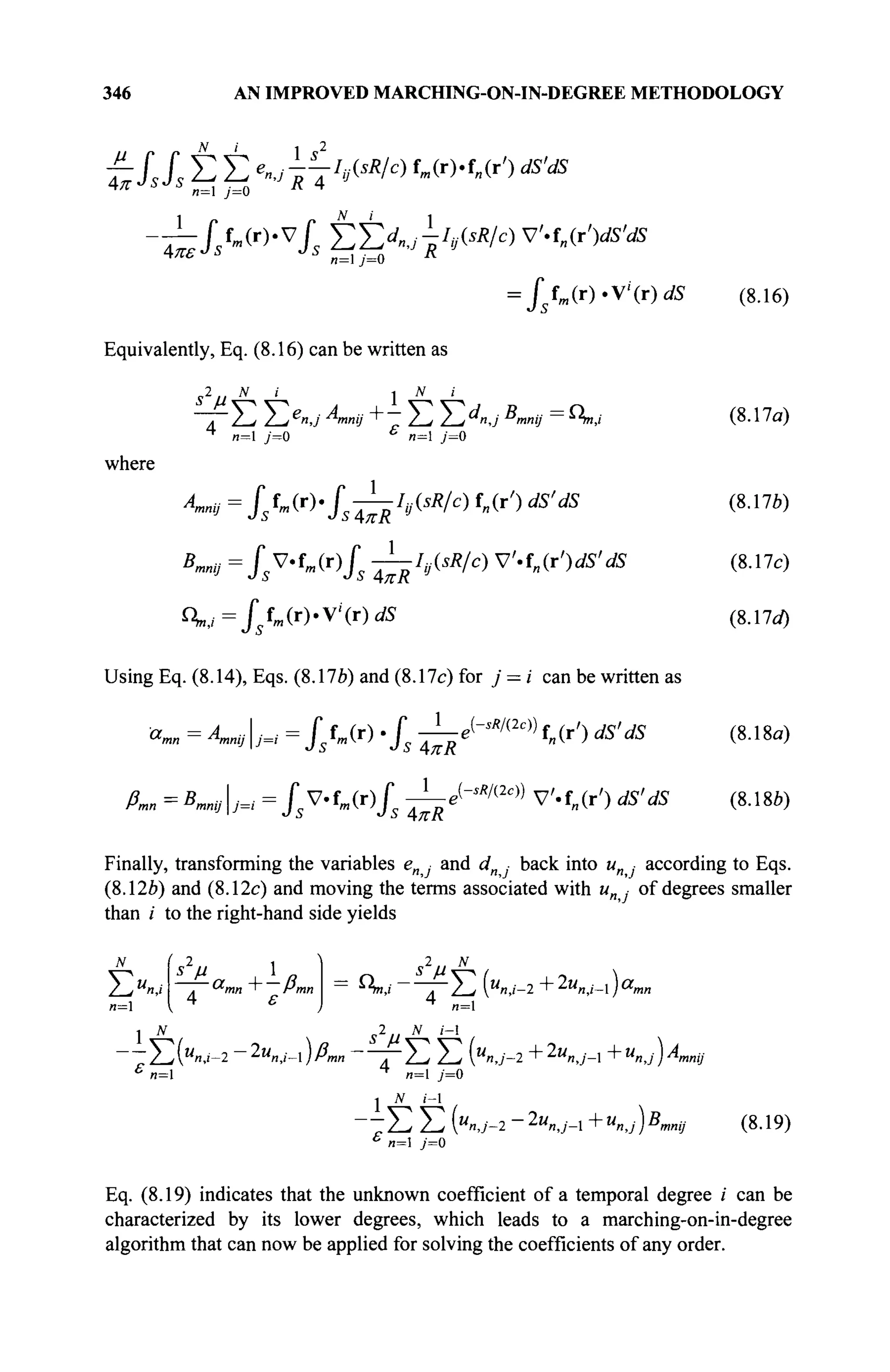
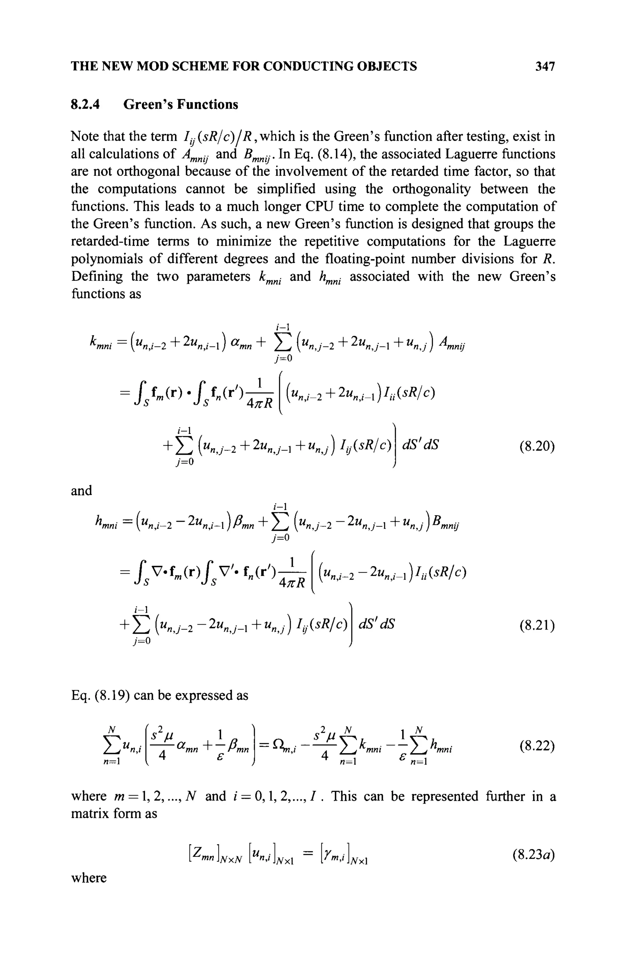
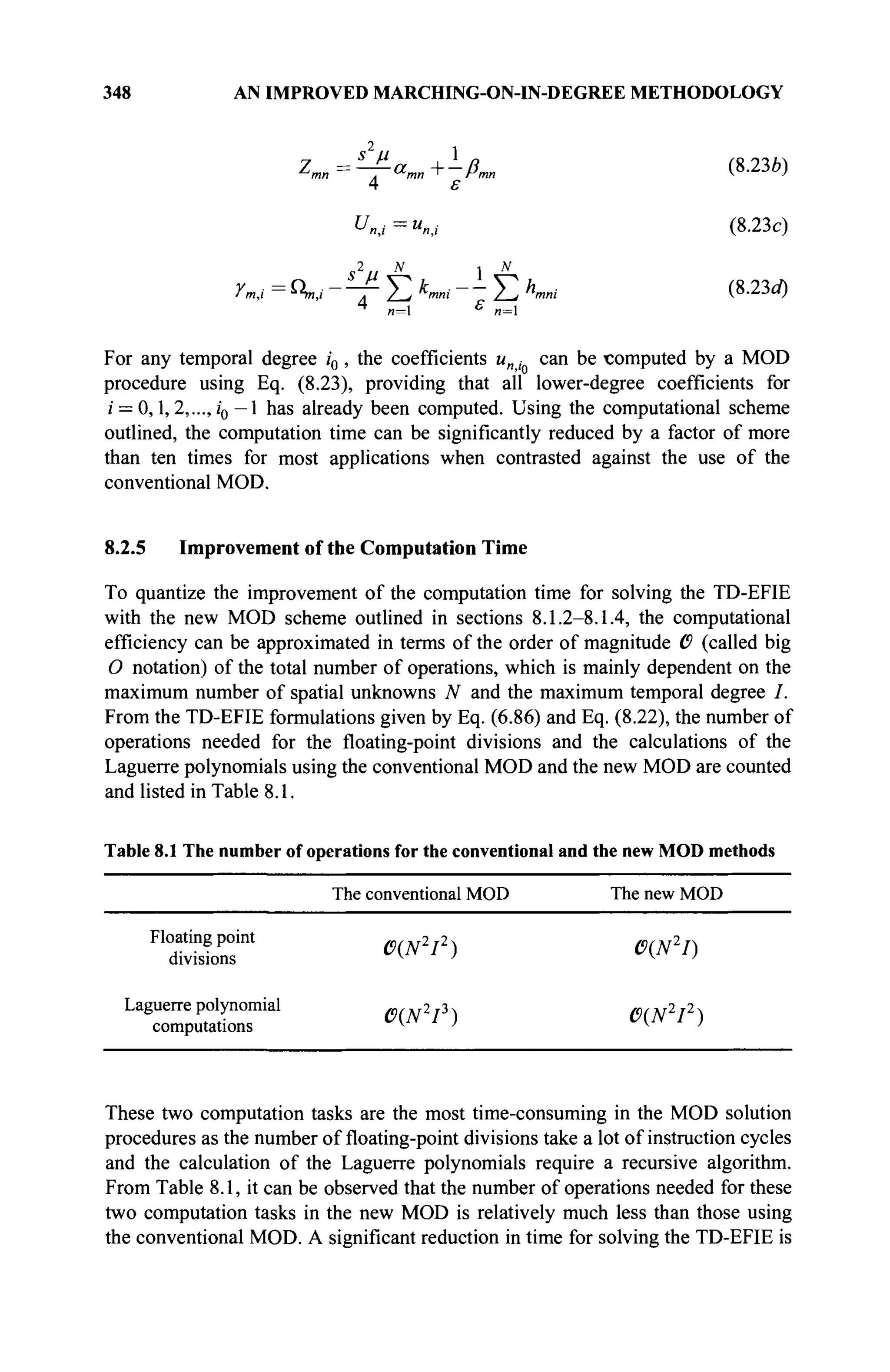
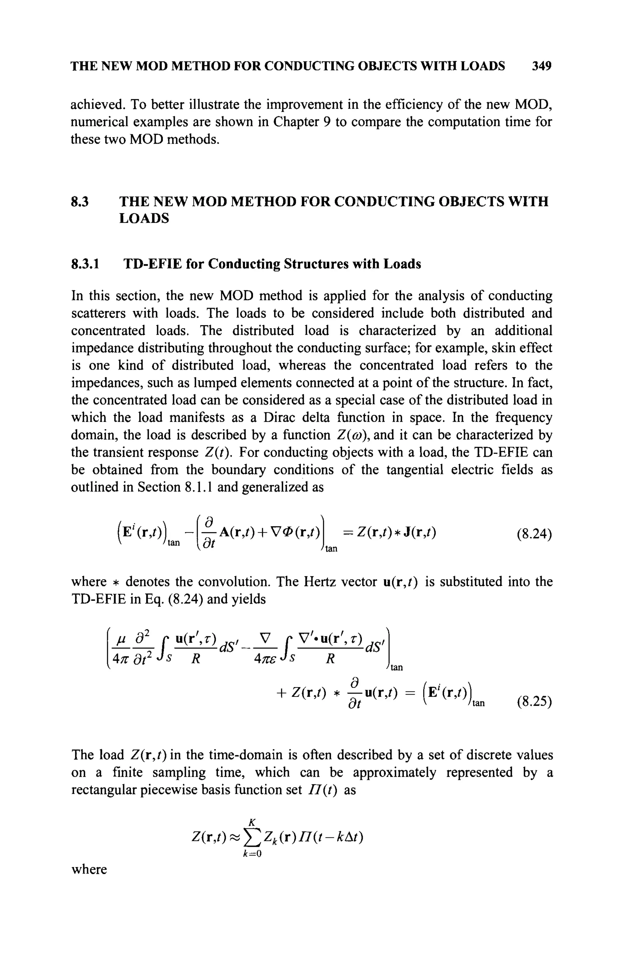
![350 AN IMPROVED MARCHING-ON-IN-DEGREE METHODOLOGY
/7(0 =
1 0 < t < Δί
0 others
(8.26)
If At is chosen small enough, then the convolution of the load Z(r,t) with the
current J(r,/) is given by
Z(iy) * -f- u(r, г) = Σ Zk (r) | - u(r, t - кAt)
3t f^0 dt
(8.27)
8.3.2 Expansion Procedures
Following the similar procedures described in Section 8.1.2, the TD-EFIE in Eq.
(8.25) can be expanded by the spatial basis function set f„(r) and the temporal
basis function set ф} (st) — 2^ ·+1 (st) + φ^+2 (st), respectively, and yields
N 00
4 π A
и=1 7=0 K Щ
™ „ N oo i
L Σ Σ,^-(φ^)-2φ^τ) + φ]+2(5τ)) V'.f„(r') dS'
4πε
κ
=1 7=0
N OO
-Σ ζ,(ν)Σ Σ -иПг](Ф№-*ш)-ф]+2&-8Ш)) f„(r)
4=0 п= 7=0
(Е''(г,/)) (8.28)
Using the parameters e„ ■ and dnj defined in Eqs. (8.12Й) and (8.12c) and
assuming that м · = 0 for j < 0, Eq. (8.28) is written as
/; n N
°° 1 e2
— f У УЧ /-—*/(«■) f„(r') ds'
4л· ε
r λ
XEÇ^,7^(^)V'-f„(rV5'
/1=1 7=0
Л IS OO
/1=0 n=l 7=0"
tan (8.29)](https://image.slidesharecdn.com/timeandfrequencydomainsolutionsofemproblemsusingintegralequationsandahybridmethodologyb-250205130750-568a5ba2/75/Time-and-Frequency-Domain-Solutions-of-EM-Problems-Using-Integral-Equations-and-a-Hybrid-Methodology-B-H-Jung-pdf-370-2048.jpg)
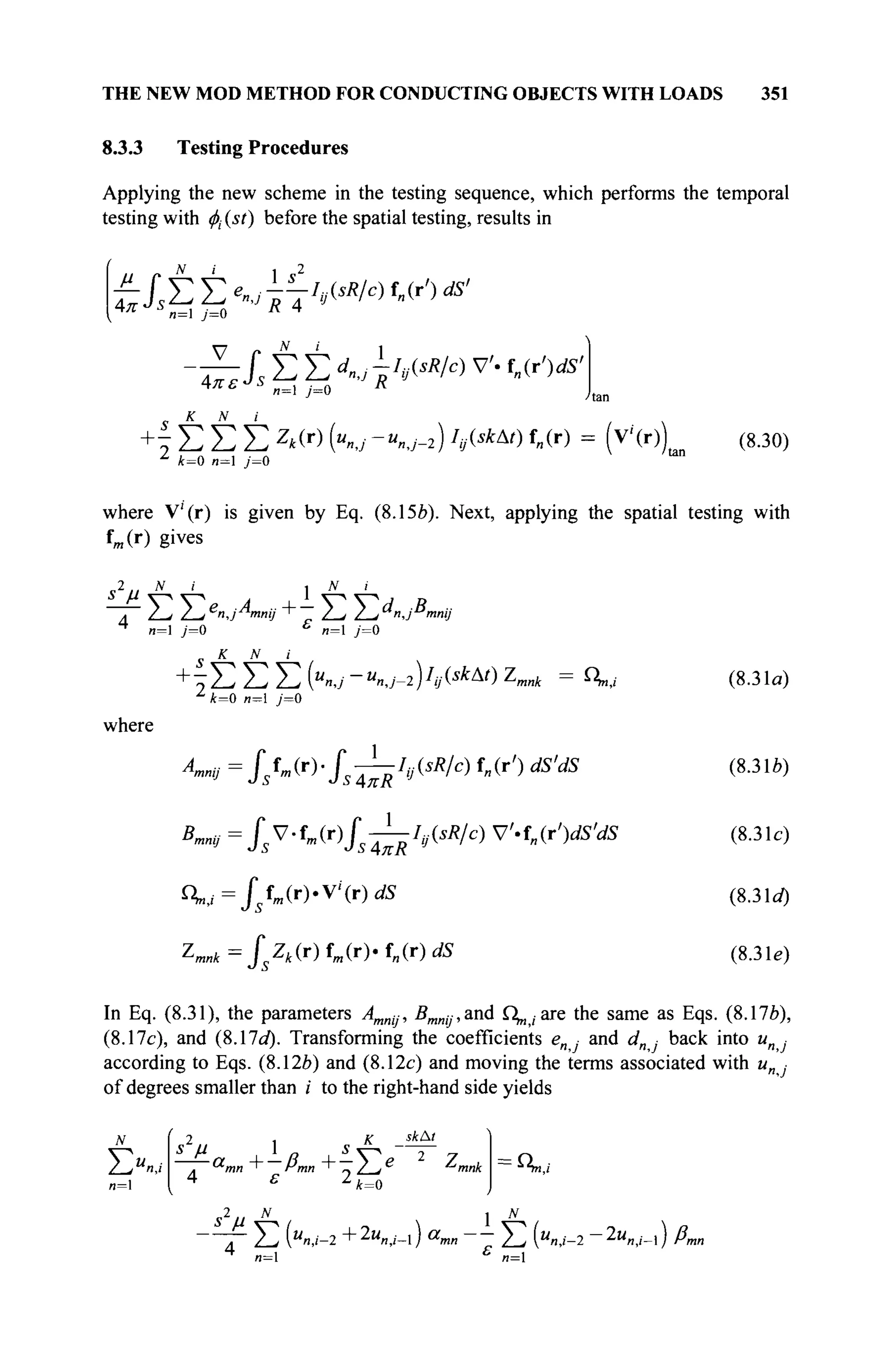

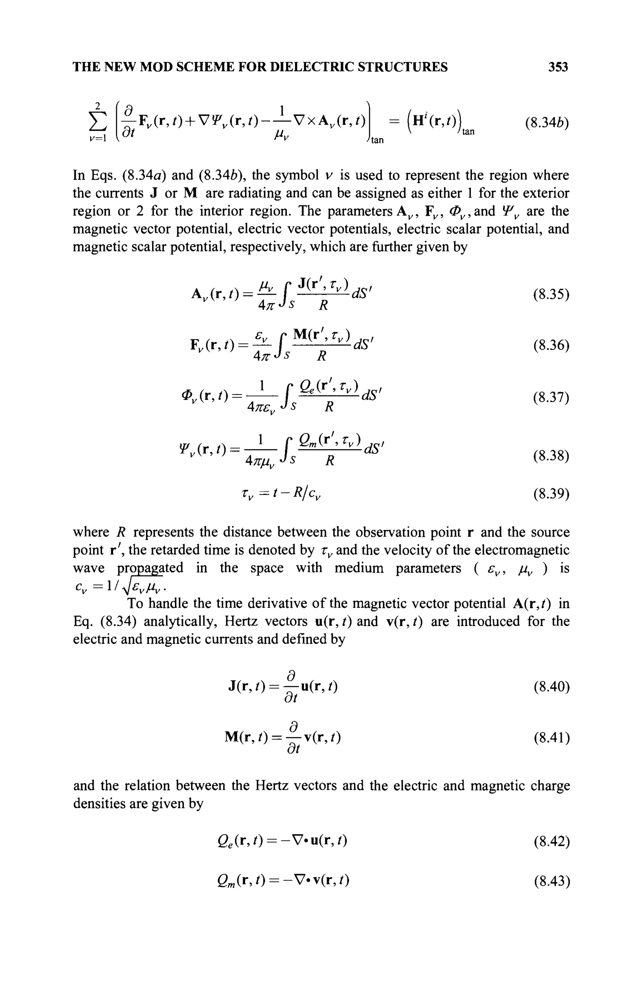
![354 AN IMPROVED MARCHING-ON-IN-DEGREE METHODOLOGY
Substituting Eq. (8.35H8.43) into Eq. (8.34), the TD-PMCHW is rewritten as
μν д2
r u(r',0 ,c, V r V'.u(r',/) ,_,
2
Σ
v=
■I. -dS' —
/
V «u(r
s R
dS'
4π dt2 J s
R 4πελ
1 С „ r
Vx
Απ r)t J S
Απδί Js R
έ ί 4πδί2
^ R 4πμν
= (E''(r,r))
ν=1
г, ô2
r v(r',/) w V
Г V'.v(r',0 w
-dS r V «v(r
s,
-dS'
4л· ö/ J 5 Л
-ctf' (Η'(Γ,Ο)
(8.44)
(8.45)
8.4.2 Expansion Functions
These unknown Hertz vectors u(r, t) and v(r, t) are spatially expanded by the
RWG vector function set f„ (r) as
N
u(iv) = I > „ W f „ ( r )
v(r,i) = t v „ ( i ) f „ ( r )
(8.46)
(8.47)
n=l
and the transient coefficients in Eqs. (8.46) and (8.47) are further expanded by
using the new temporal basis function φ, (st) — 2φ,+λ (st) + φ:+2 (st). One obtains
oo
M O = Σ Μ (Φ№)-2φι+χ^ί) + φ]+2^ί)) (8.48)
oo
К (0 = Σ v
«J К (*') - 2
^'+i (*') + ^'+2 (*')) (8.49)
Substituting Eqs. (8.46H8.48) into Eqs. (8.44) and (8.45) results in
Σ 4π
N 1 oo 2
Σίΐτ £".j7^w+^i(i(
)H+2M)i,(r') «я'
n=l iv
y=0
Л I 00
V
Σί -E«»,;feH-2^M +^Hv'.f„(r')Ä'
4я»„ ^ J s R
U](https://image.slidesharecdn.com/timeandfrequencydomainsolutionsofemproblemsusingintegralequationsandahybridmethodologyb-250205130750-568a5ba2/75/Time-and-Frequency-Domain-Solutions-of-EM-Problems-Using-Integral-Equations-and-a-Hybrid-Methodology-B-H-Jung-pdf-374-2048.jpg)
![THE NEW MOD SCHEME FOR DIELECTRIC STRUCTURES 355
i ΛΓ -I oo
+^ν χ
Σ/5 - Σ ^ Λ ^ ο - ^ Η ^ ο ^ '
( Ε
' ' Μ . η (8
·50)
and
2
Σ
v=l
[τΣ Jl ^ Σ ν Α Κ ^ + ^+.^ + ^ Η f„(r') dS'
i iV . 1 oo
" 1 — V
Σ L -Σνη^{3ί)-2φ]+λ{*ί) + φ]+2{*ί)) V'.f„(r') dS'
■V и=1 y=o
i л i oo
л=1 JV
y=0
8.4.3 Testing Functions
(Η'(Γ,Ο)
V /ti
(8.51)
Following the testing procedures described in Section 8.1.3, Eq. (8.51) is tested in
time with φί (st) first and then, defining td = sR/c, yields
2
Σ
v=l
4πε,
I· 14 Г ] V
Τ " Σ L 7E«n.;T (^ar f ) + 2Vi(/r f ) +V2(^))fH(r') ^ '
1 N „ ι oo
V V
Σ / , ^ I X j ( W - 4 y + i ( ^ + W ' ' ) ) V
4 ( r ' ) ^ '
ι ΛΡ I oo
+^νχ
Σ/5 ^ vy(№)-wo))f„(r')л'
j~° /tan
= (V
'<r
>L (8
·52
«)
Vf(r)= Г 4(*/)Е'(г,0</(*0 (8.52ft)
*/ О
where
and
Σ
f N
p 1 °° o2
n=l Jv
y=0
1 /V 1 00
- ^ - V
Σ £ ^ Σ ν
« Λ ¥ ^ - 2 / , V + 1 ( ^ + W ' , ) ) V'.f„(r') dS'
=1 " 7·=0](https://image.slidesharecdn.com/timeandfrequencydomainsolutionsofemproblemsusingintegralequationsandahybridmethodologyb-250205130750-568a5ba2/75/Time-and-Frequency-Domain-Solutions-of-EM-Problems-Using-Integral-Equations-and-a-Hybrid-Methodology-B-H-Jung-pdf-375-2048.jpg)
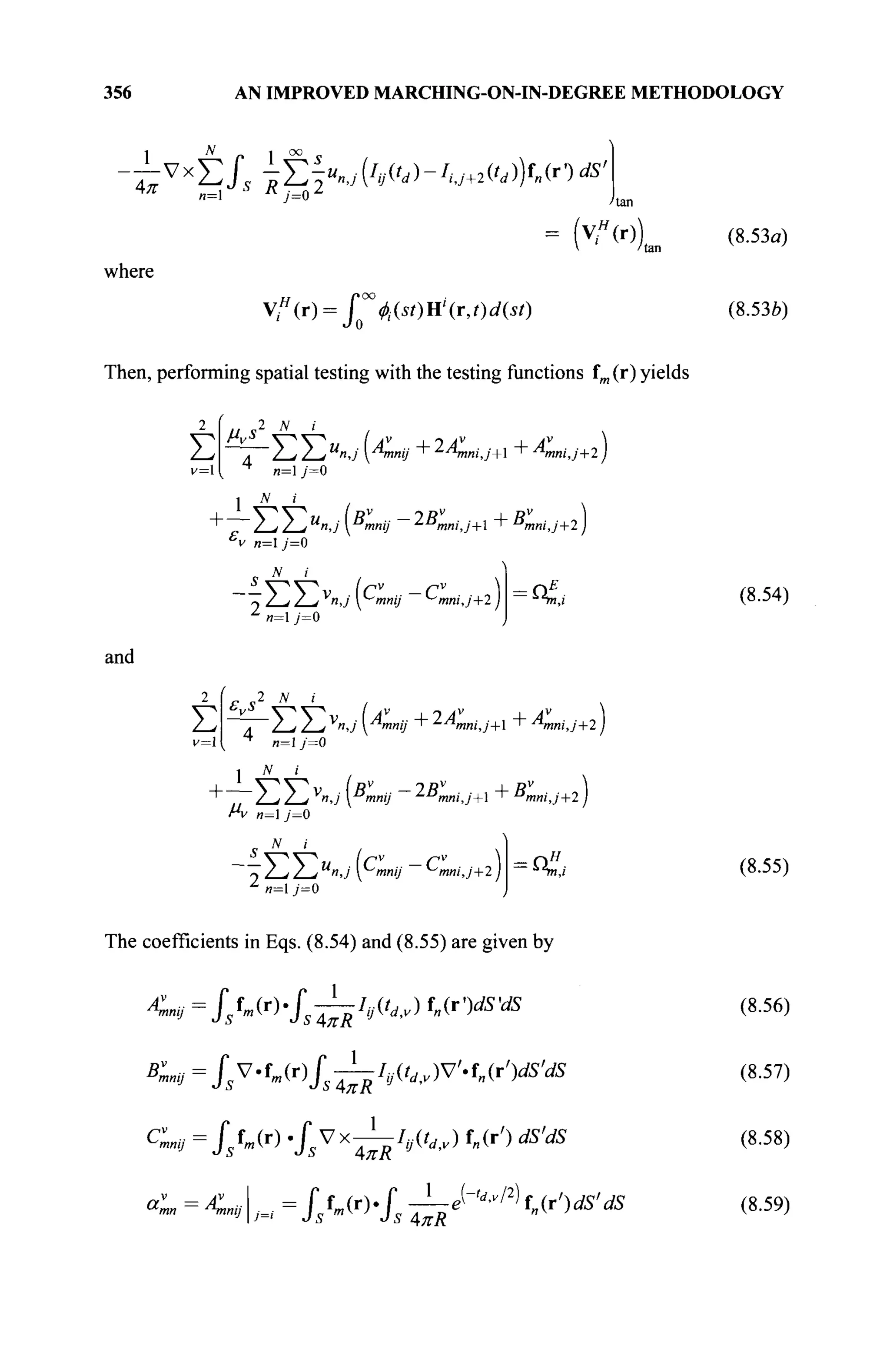
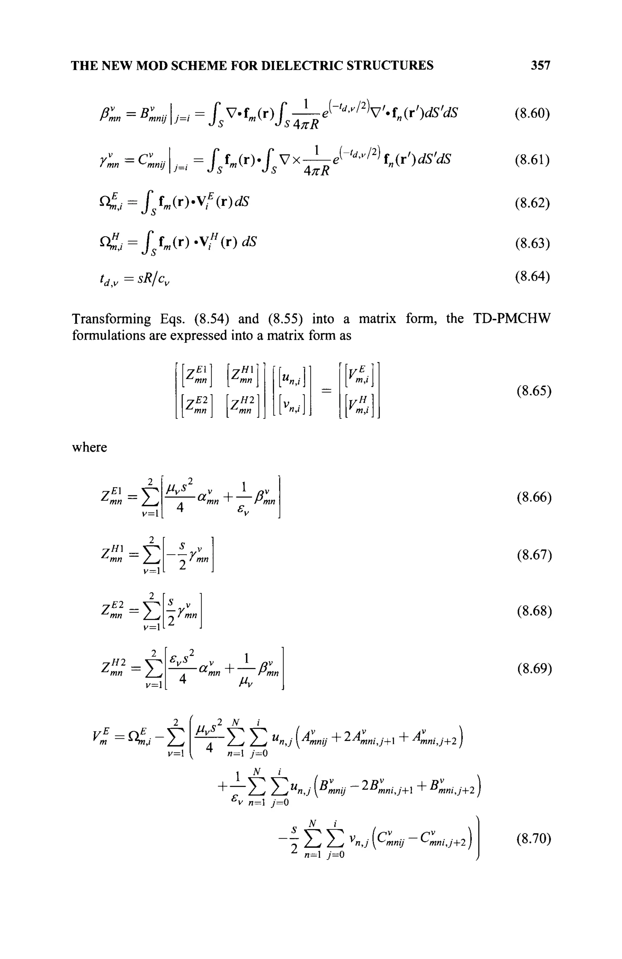
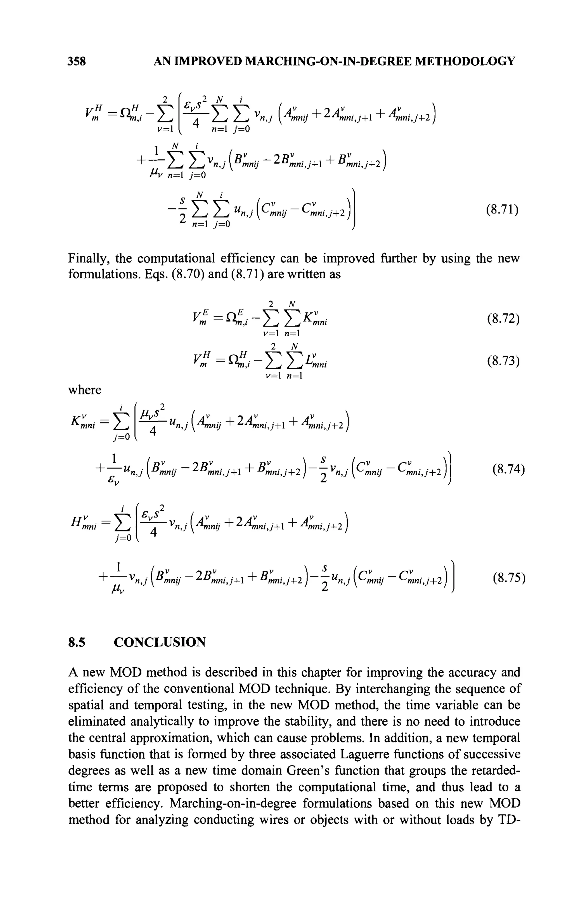
![REFERENCES 359
EFIE and dielectric objects by TD-PMCHW are presented. Numerical examples
will be given in Chapter 9 to demonstrate the effectiveness of these improvements.
REFERENCES
[1] E. A. Essex, "Hertz vector potentials of electromagnetic theory," Am. J. Phys.,
Vol. 45, pp. 1099-1101,1977.
[2] Z. Ji, T. K. Sarkar, B. H. Jung, Y.-S. Chung, M. Salazar-Palma, and M. Yuan, "A
stable solution of time domain electric field integral equation for thin-wire
antennas using the Laguerre polynomials, " IEEE Trans. Antennas Prop., Vol. 52,
pp. 2641-2649, 2004.
[3] Z. Ji, T. K. Sarkar, B. H. Jung, M. Yuan, and M. Salazar-Palma, "Solving time
domain electric field integral equation without the time variable," IEEE Trans.
Antennas Prop., Vol. 54, pp. 258-262, 2006.
[4] Z. Mei, Y. Zhang, T. K. Sarkar, "Solving time domain EFIE using higher order
basis functions and marching-on-in-degree method," Anten. Prop. Society Int.
Sym., 2009, 2009.
[5] D. Poularikas, The Transforms and Applications Handbook, IEEE Press,
Piscataway, N.J., 1996.
[6] N. N. Lebedev, Special Functions and Their Applications, Prentice-Hall,
Englewood Cliffs, N.J., 1963.
[7] B. G. Mikhailenko, "Spectral Laguerre method for the approximate
solution of time dependent problems," Appl. Math. Lett., Vol. 12, pp.
105-110,1999.](https://image.slidesharecdn.com/timeandfrequencydomainsolutionsofemproblemsusingintegralequationsandahybridmethodologyb-250205130750-568a5ba2/75/Time-and-Frequency-Domain-Solutions-of-EM-Problems-Using-Integral-Equations-and-a-Hybrid-Methodology-B-H-Jung-pdf-379-2048.jpg)
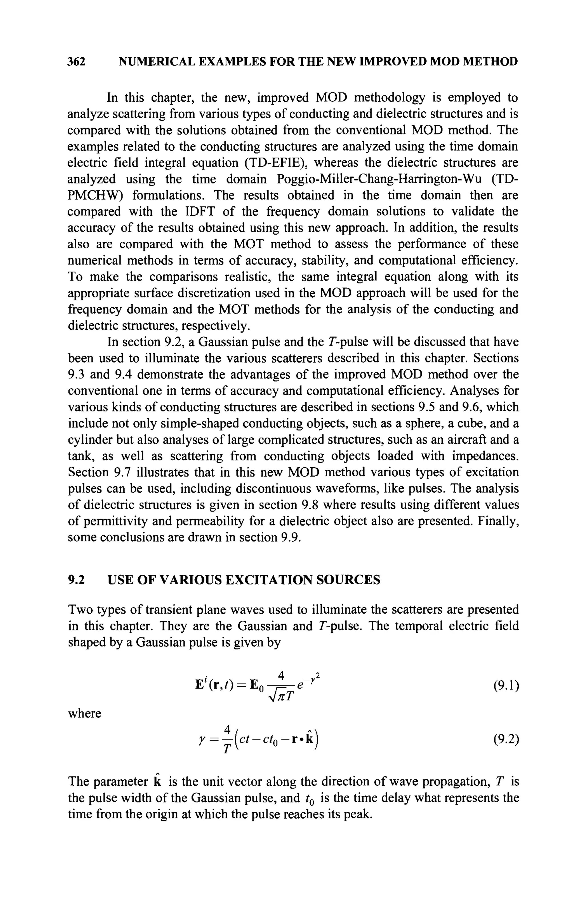
![USE OF VARIOUS EXCITATION SOURCES 363
The Г-pulse is a discrete time signal with most of its prescribed energy
focused in a given bandwidth [1]. It is a strictly time-limited pulse with the added
stipulation that 99% of its signal energy be concentrated in a narrow band. Hence,
effectively, the pulse is also approximately band limited. In addition, the pulse can
be designed to be orthogonal with its shifted version as well and can have a zero
DC bias if required. By interpolating this discrete pulse, a continuous pulse can be
generated while its bandwidth remains approximately the same. The mathematical
generation of a Г-pulse is described in [2]. Figure 9.1 shows the transient and
frequency responses of a Г-pulse, which is 6 light-meters (lm) in duration. Most of
its energy is concentrated in the band from 0 to 200 MHz, and only less than
0.008% of the energy is out of this band so this time-limited pulse is also
practically band limited and, thus, is very convenient in system applications.
Next, responses of the system to these pulses are discussed.
2 3
Time (Im)
(«)
100 150 200
Frequency (MHz)
Figure 9.1. The Г-pulse. (a) Temporal response, (b) Spectrum.](https://image.slidesharecdn.com/timeandfrequencydomainsolutionsofemproblemsusingintegralequationsandahybridmethodologyb-250205130750-568a5ba2/75/Time-and-Frequency-Domain-Solutions-of-EM-Problems-Using-Integral-Equations-and-a-Hybrid-Methodology-B-H-Jung-pdf-382-2048.jpg)
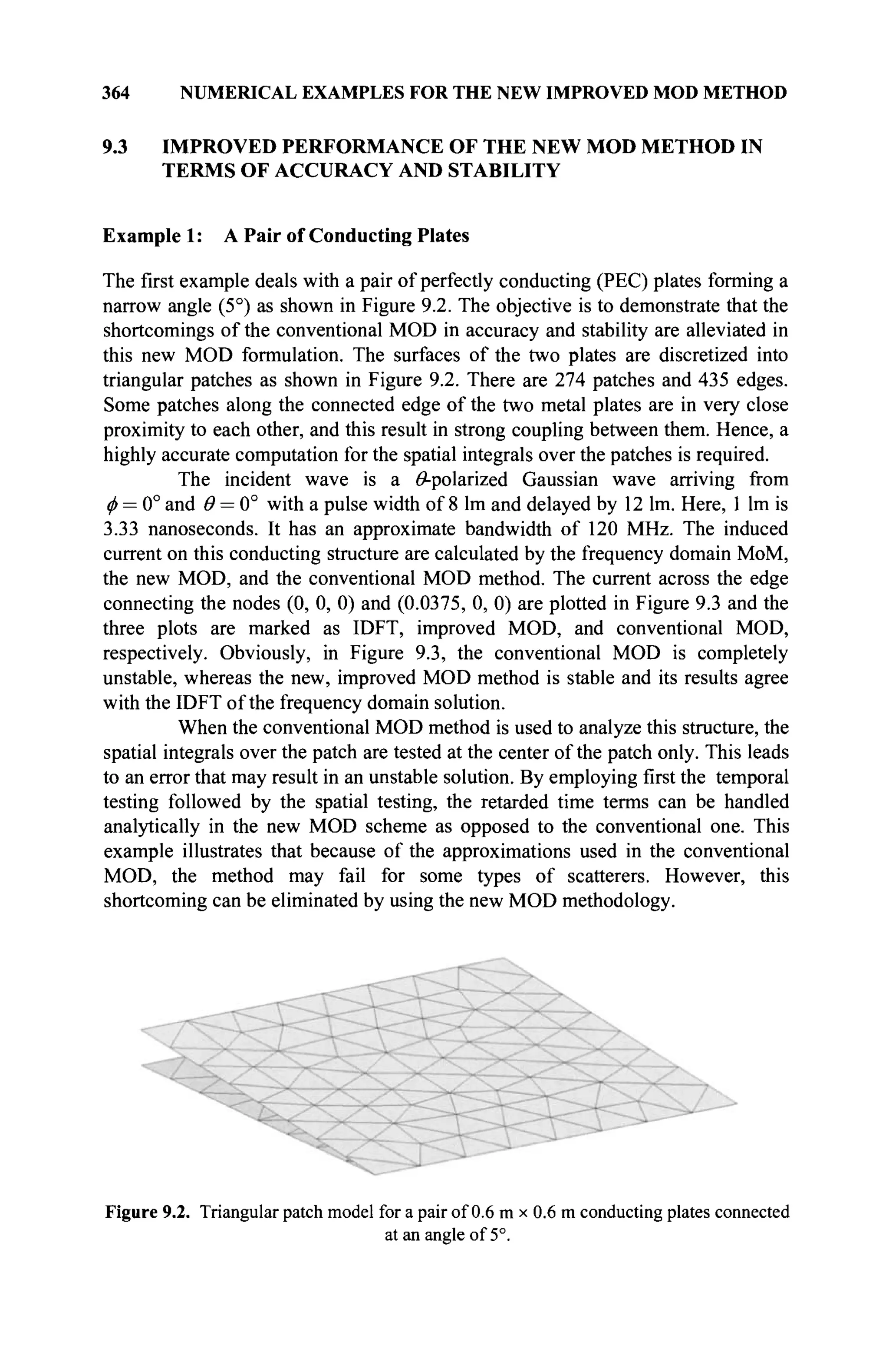
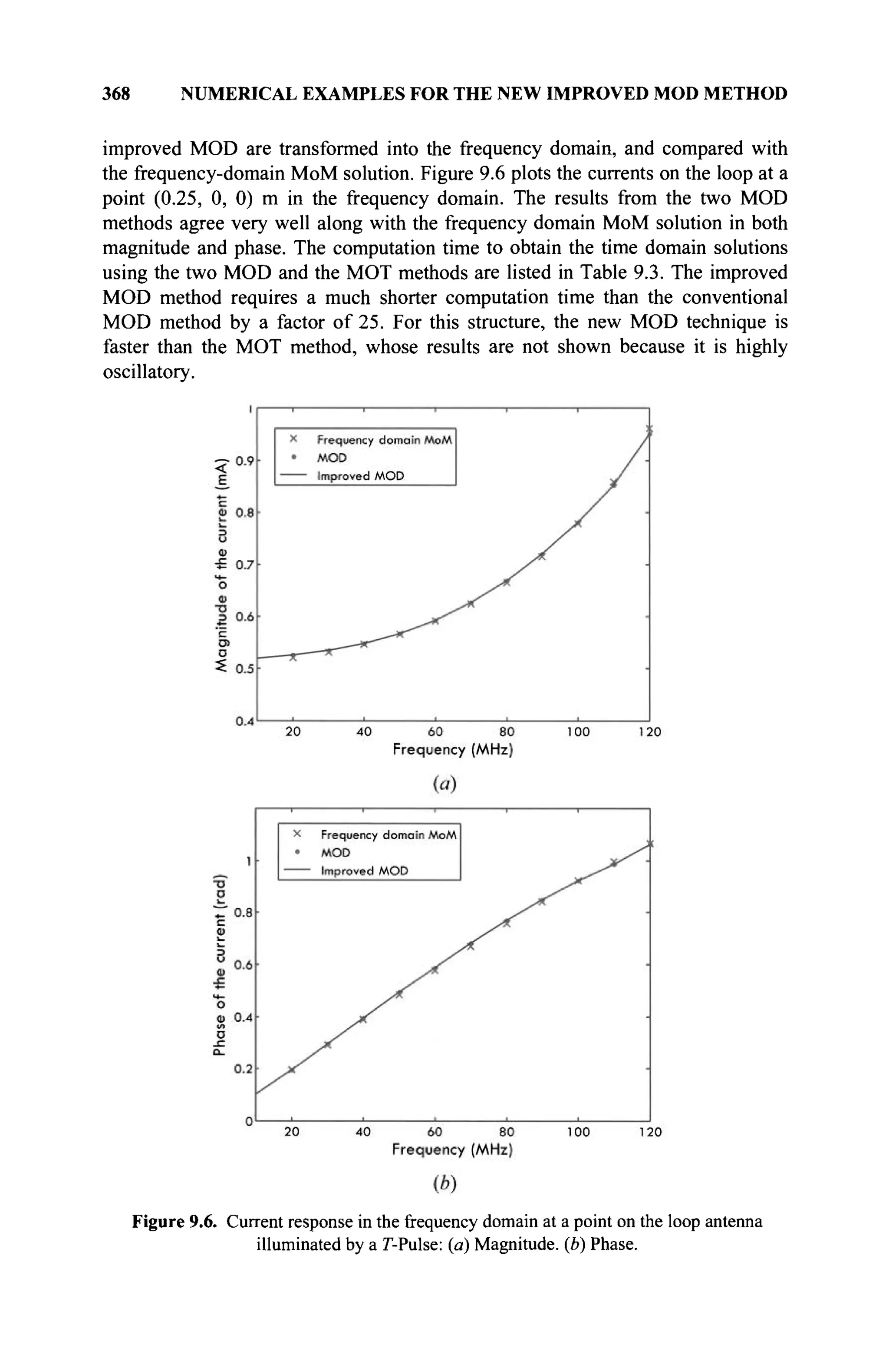
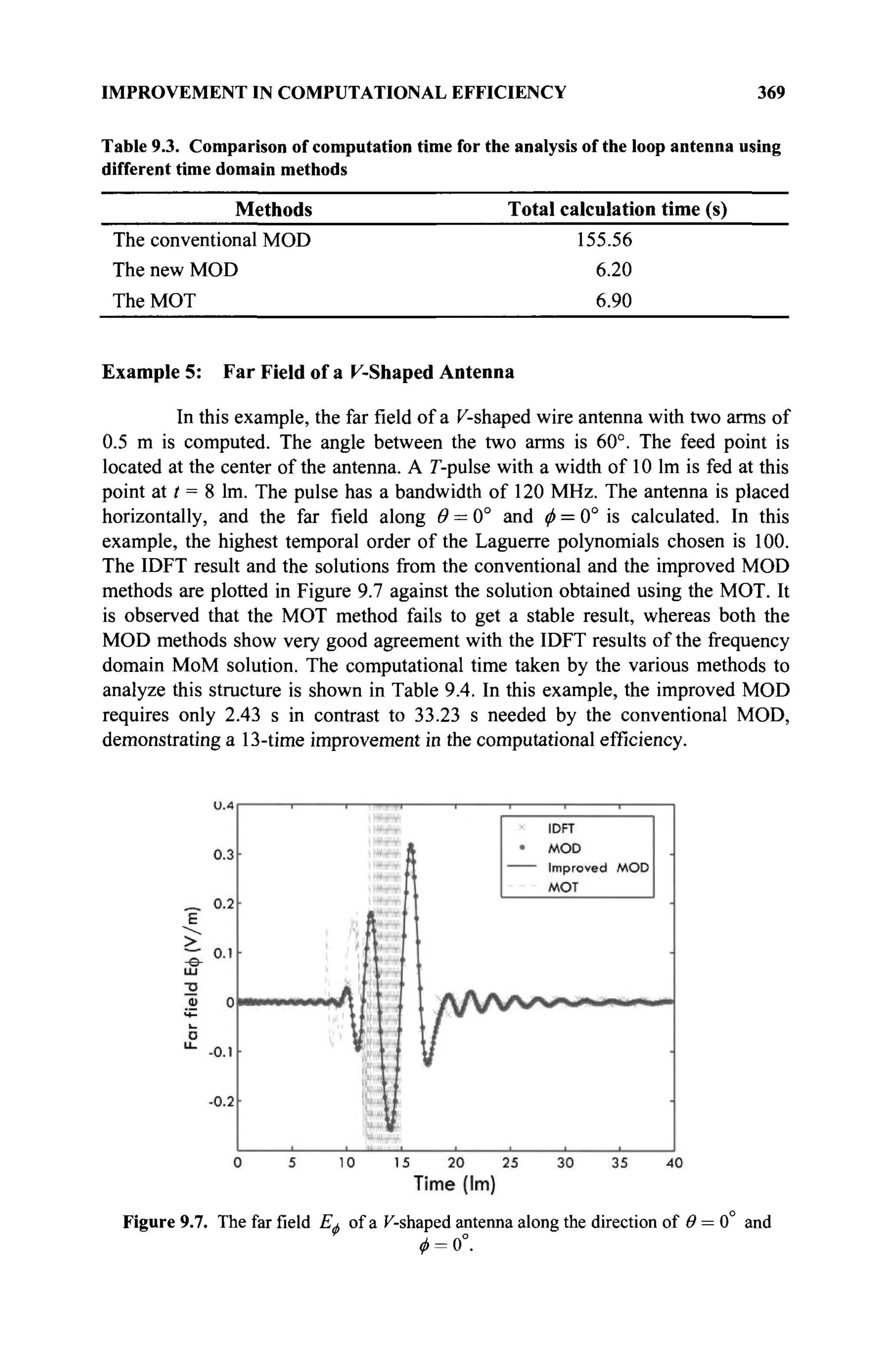
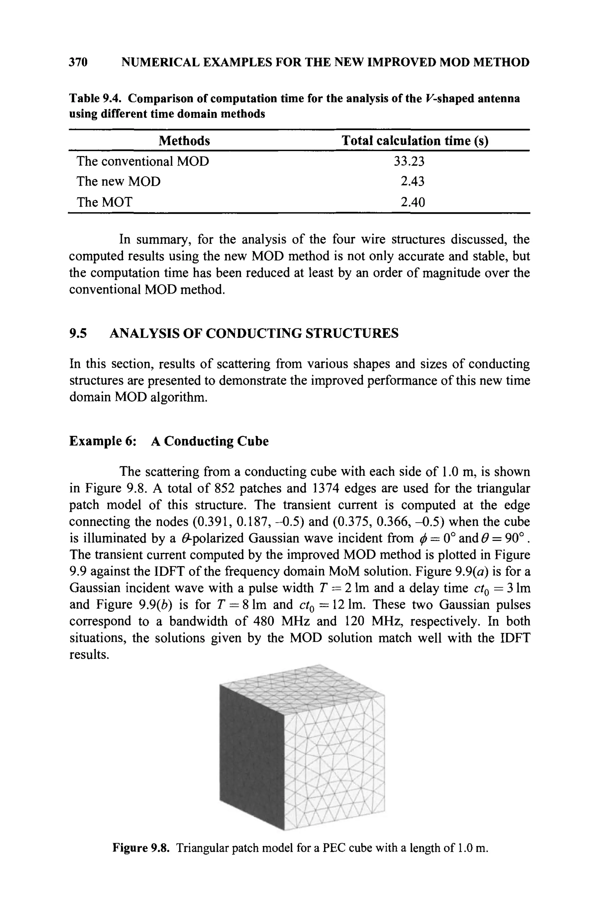
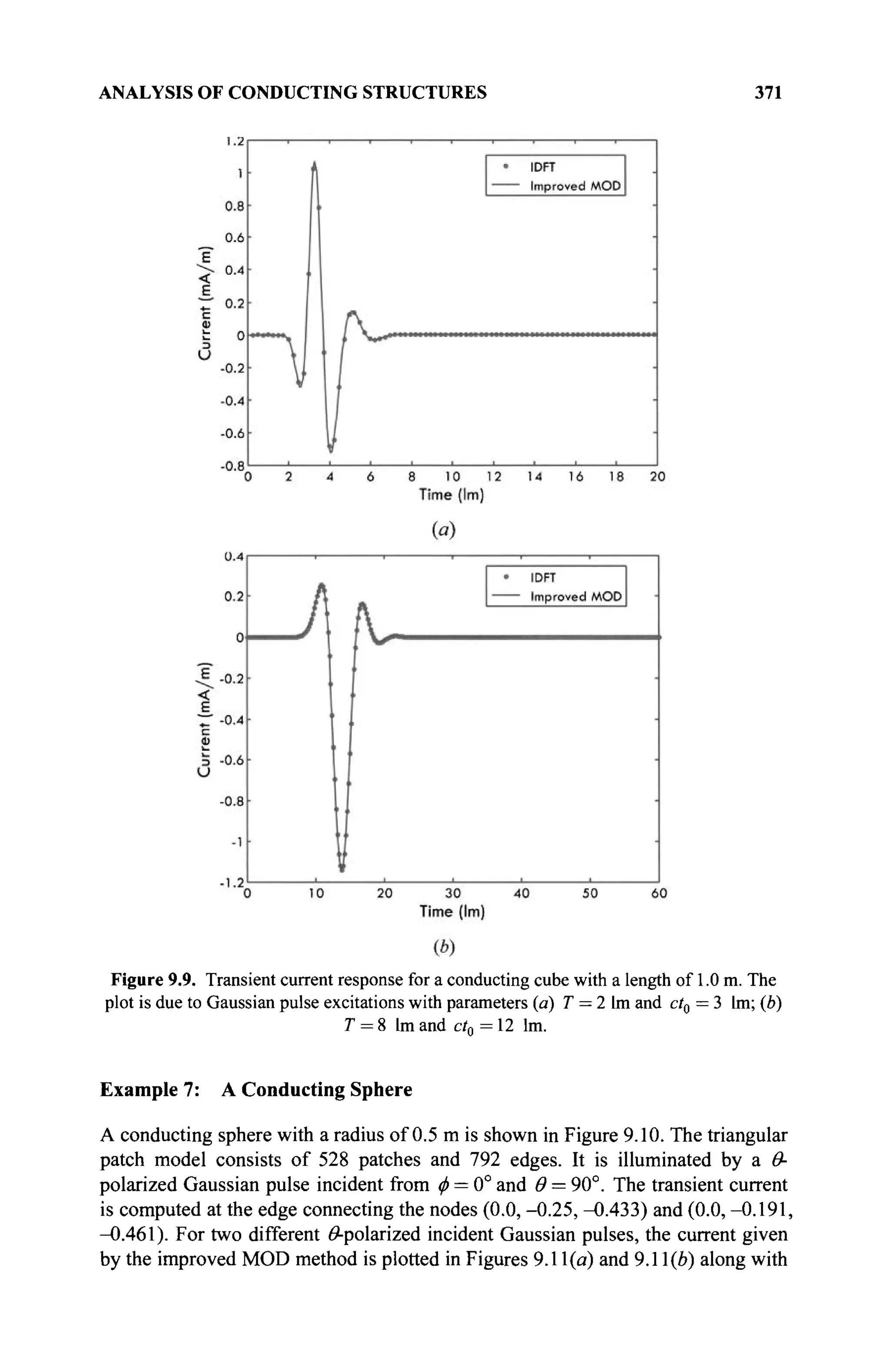
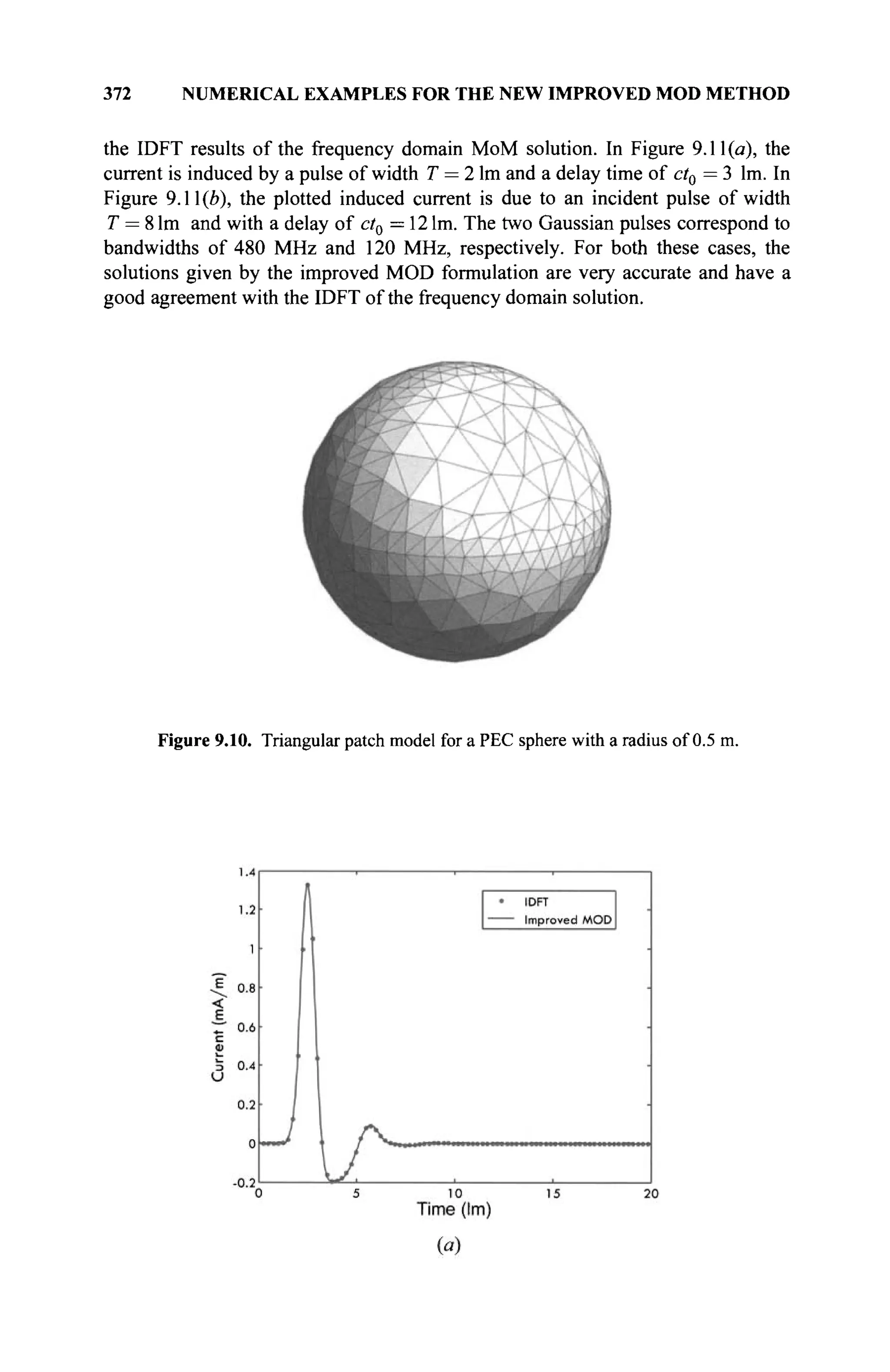
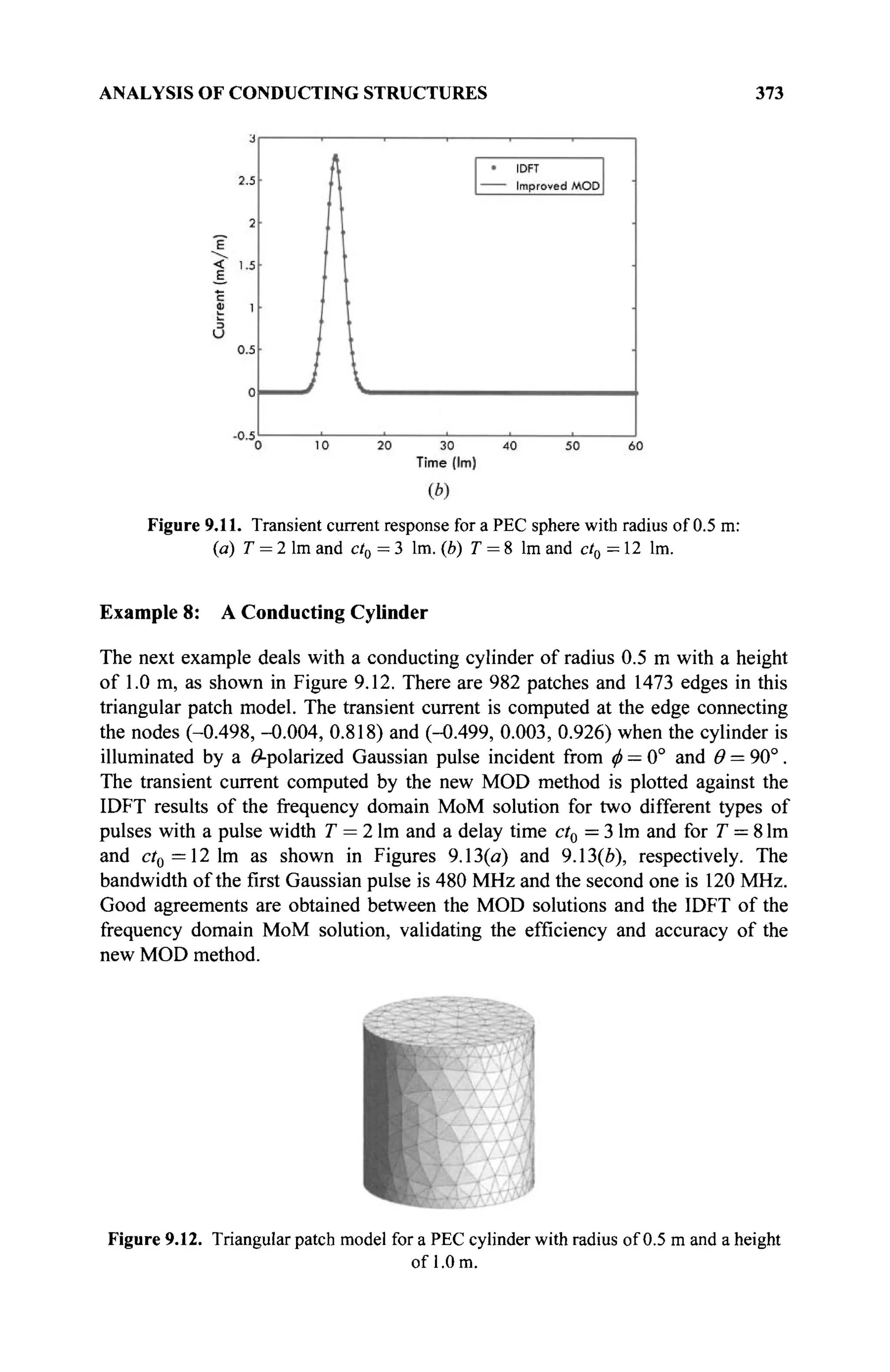
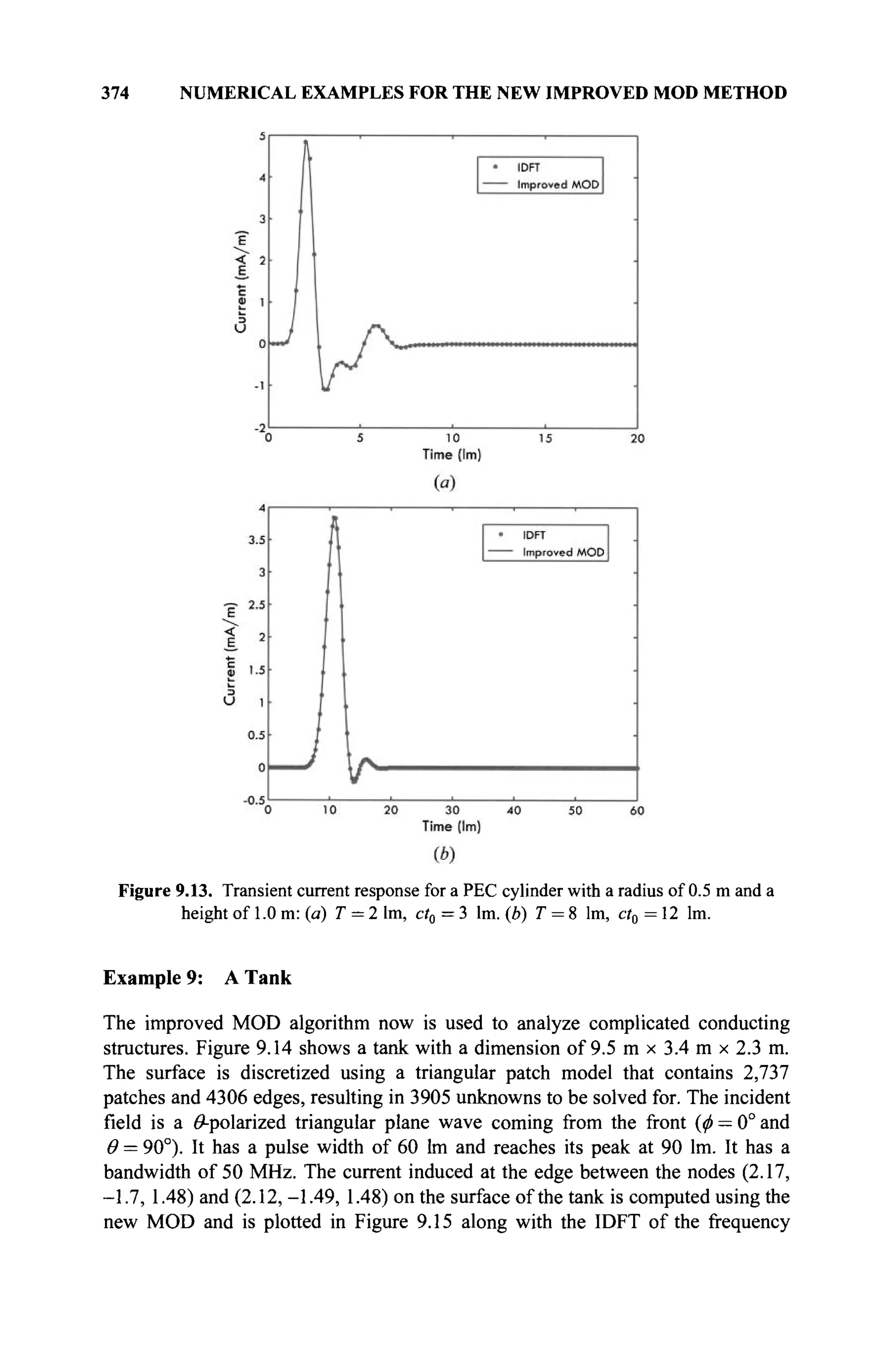
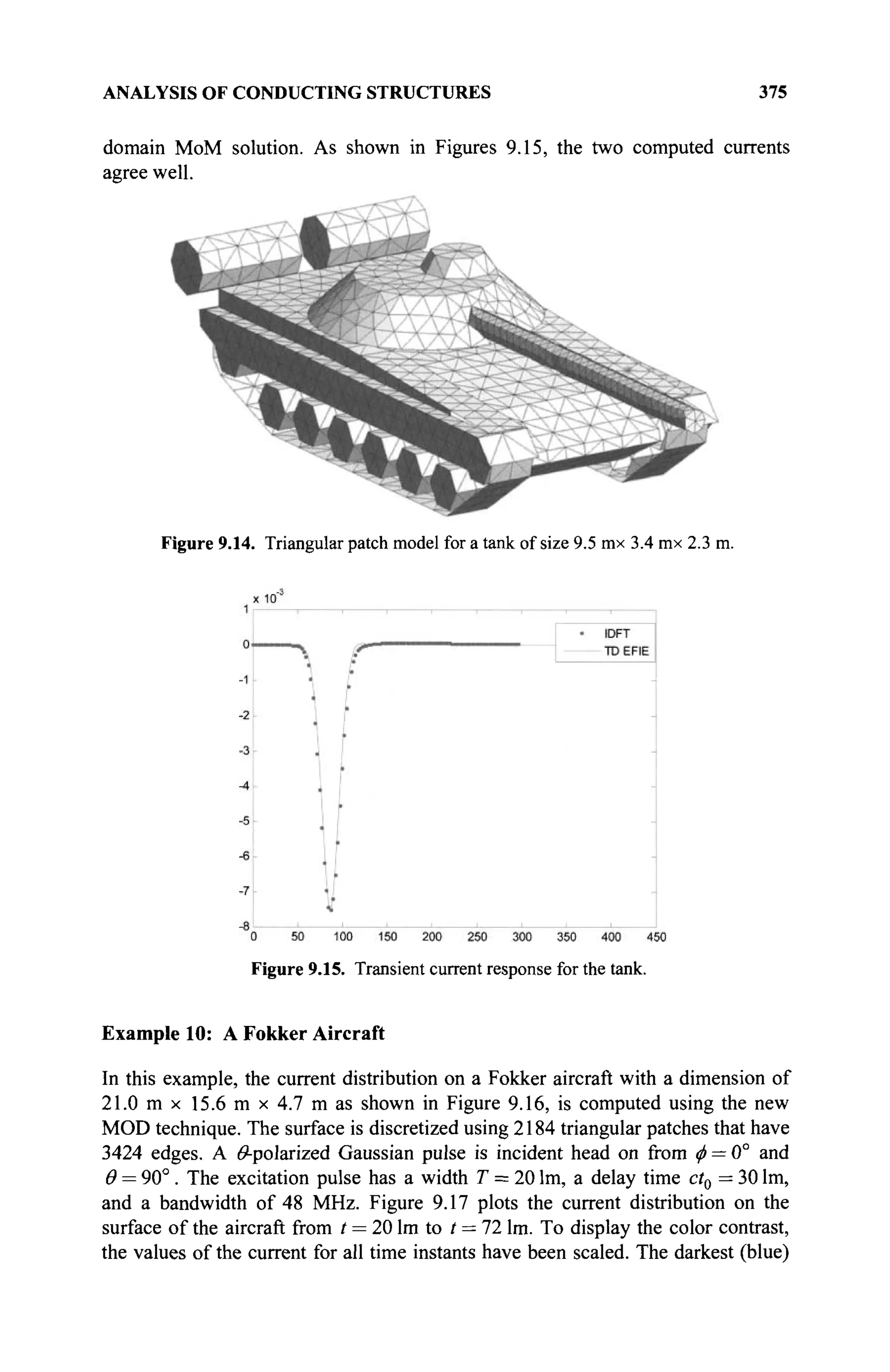
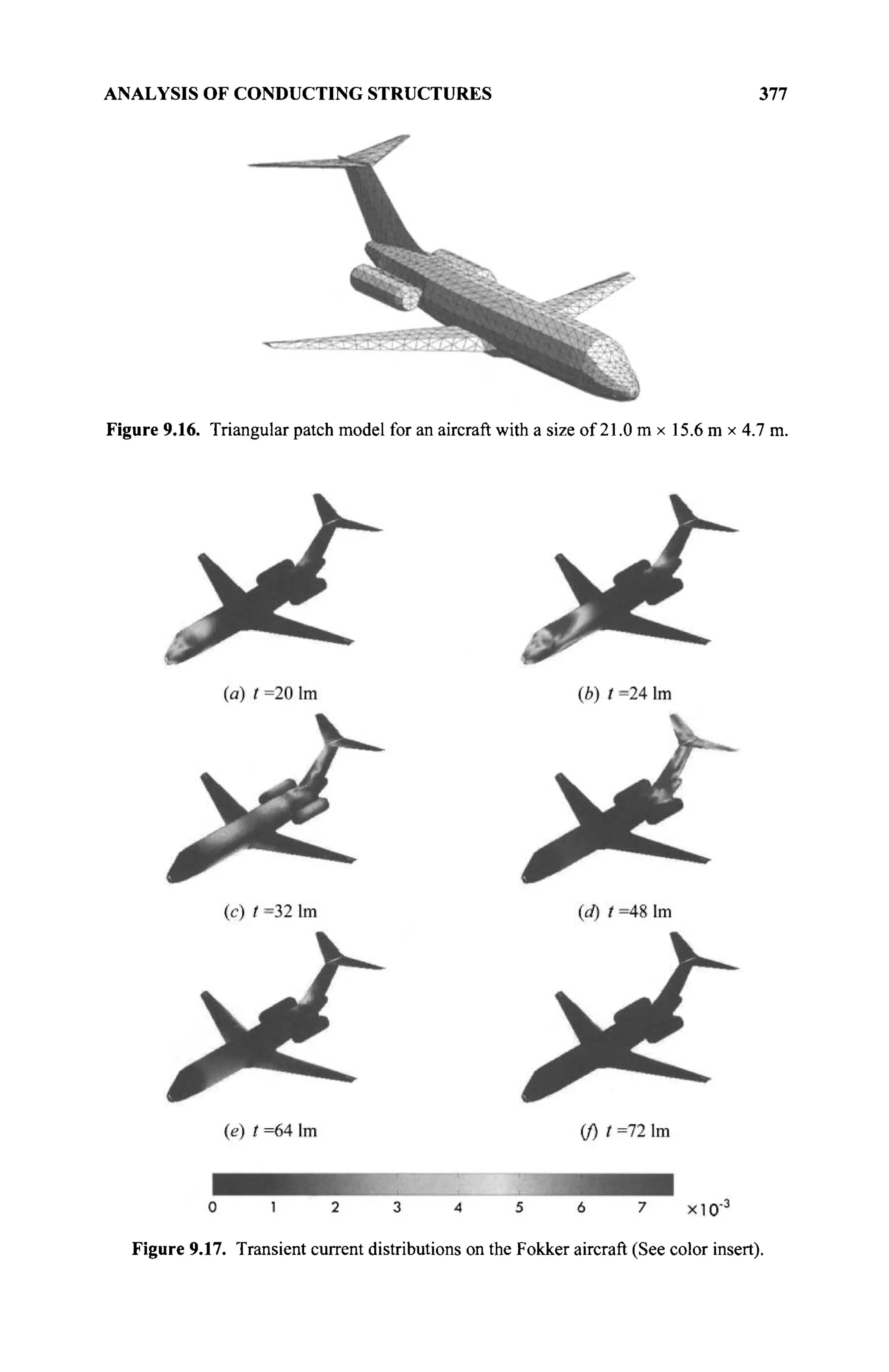
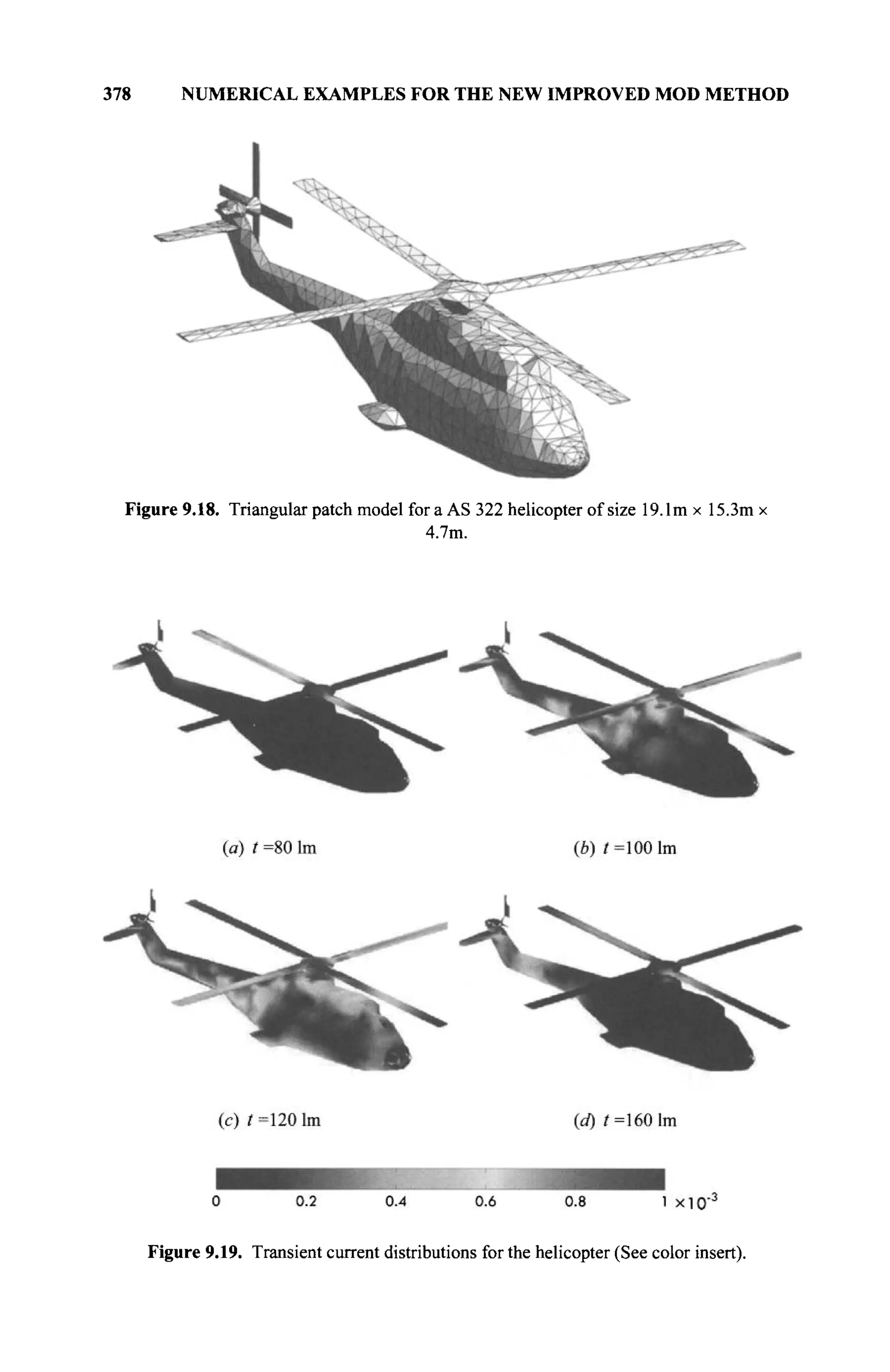
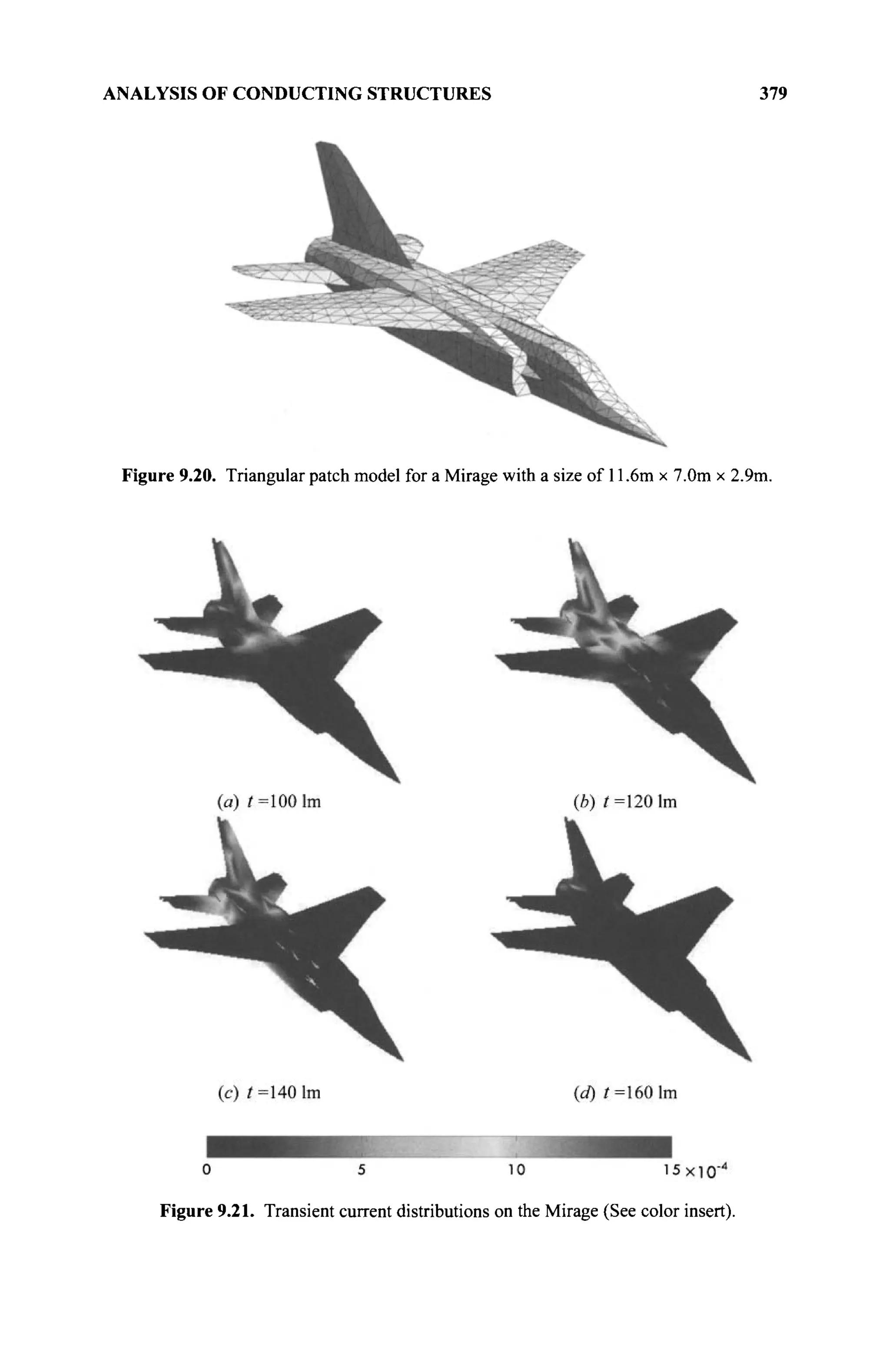
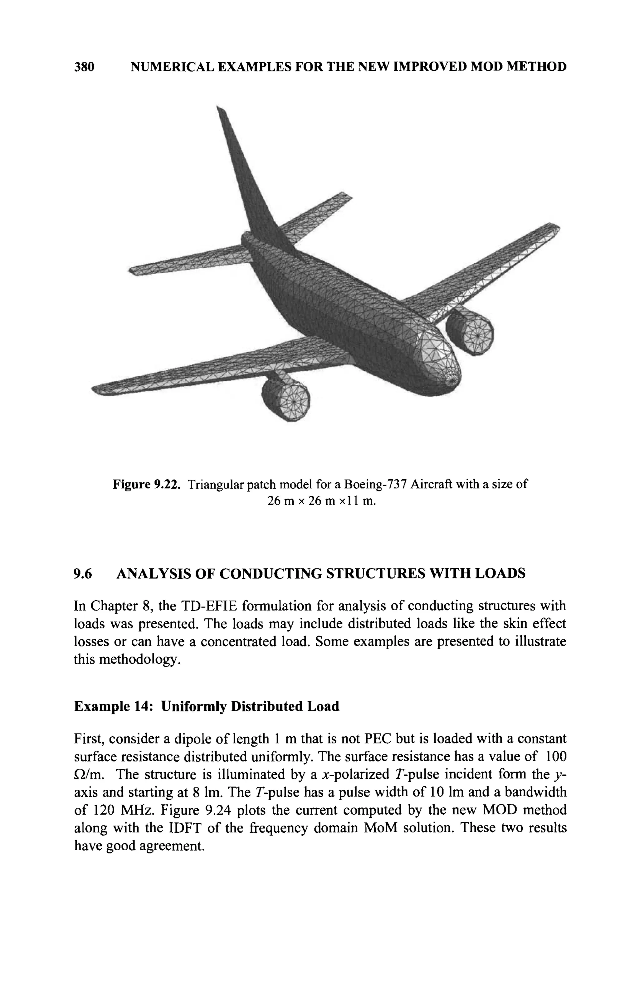
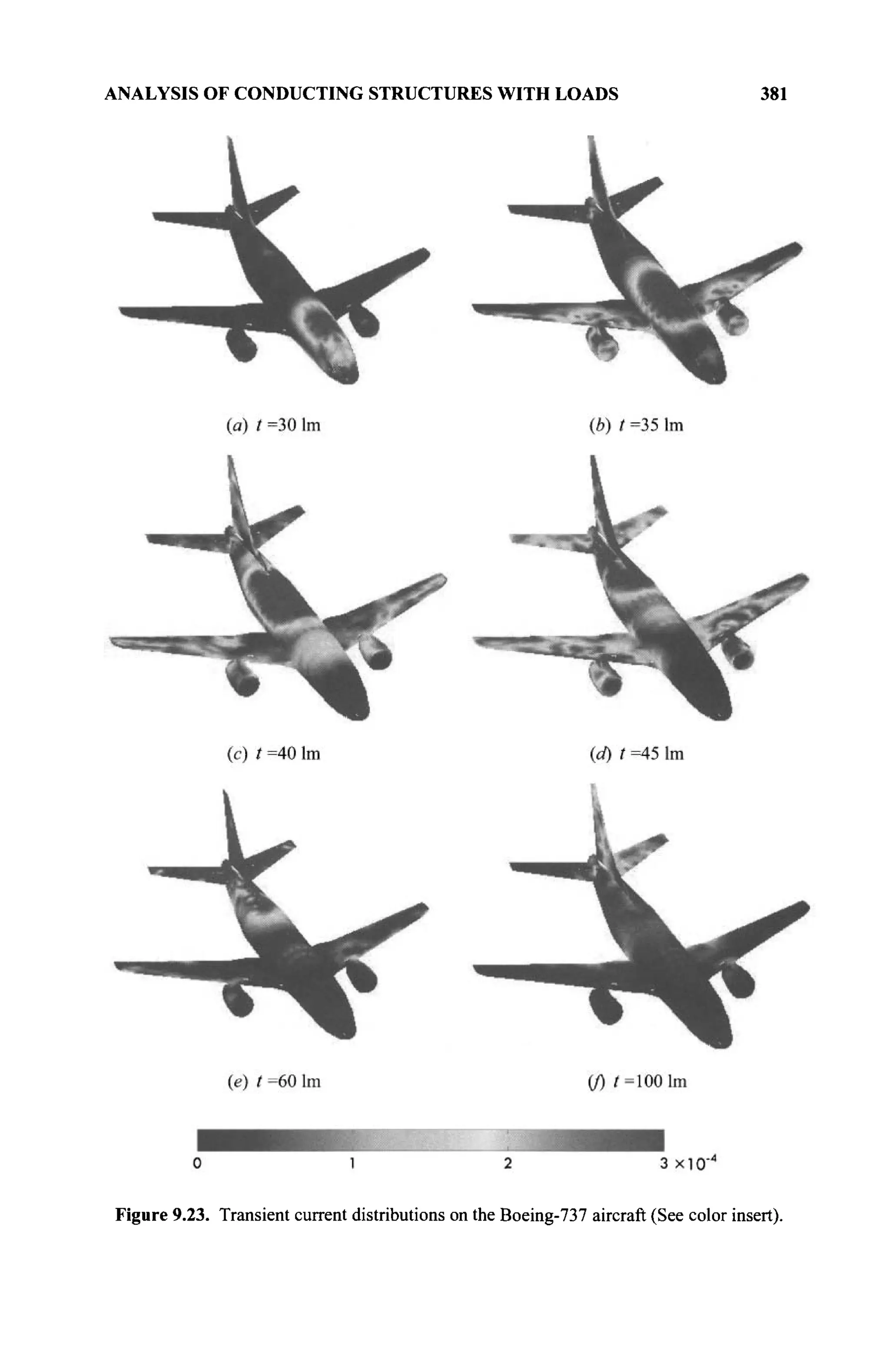
![382 NUMERICAL EXAMPLES FOR THE NEW IMPROVED MOD METHOD
0.15
0.1
0.05
0
<
-E -0.05
g -ci
и
-0.15
-0.2
-0.25
-0.3
10 15 20 25 30
Time (Im)
Figure 9.24. Transient current response on a dipole with a uniformly distributed resistance.
Example 15: Skin Effect
Skin effect is a physical phenomenon that is a result of the distribution of an
alternating electric current (AC) inside a conductor. Therefore, the cross-sectional
resistance is no longer the same like that for the direct current (DC). Particularly,
at high frequencies, most of the current is located only within a small depth h on
the skin of a conducting structure, called skin depth, which is given by
ωμσ
(9.3)
where μ is the permeability and σ is the conductivity. So the equivalent
resistance can be obtained by
Я = -^— = ±.]Л-а (9.4)
where D is the diameter of the wire.
For example, consider a 1-m dipole with a conductivity of σ — 1000 S/m.
The excitation is the same Г-pulse described in Example 14. It is x-polarized, and](https://image.slidesharecdn.com/timeandfrequencydomainsolutionsofemproblemsusingintegralequationsandahybridmethodologyb-250205130750-568a5ba2/75/Time-and-Frequency-Domain-Solutions-of-EM-Problems-Using-Integral-Equations-and-a-Hybrid-Methodology-B-H-Jung-pdf-401-2048.jpg)
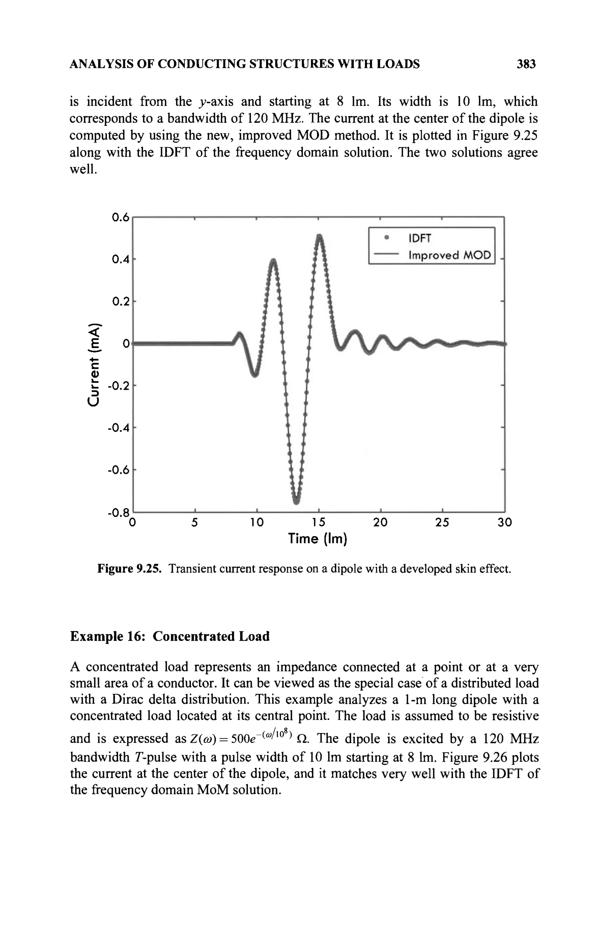
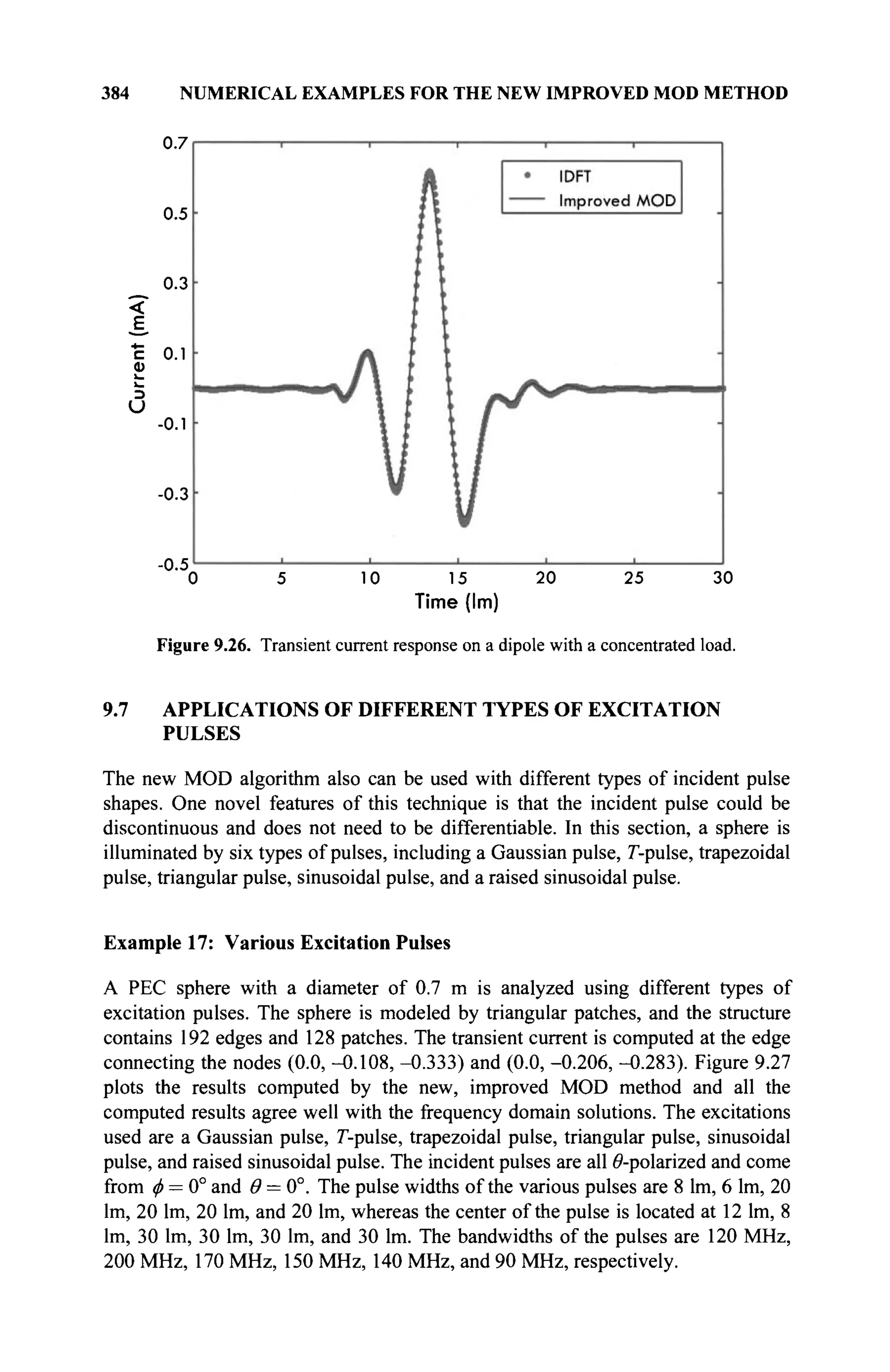
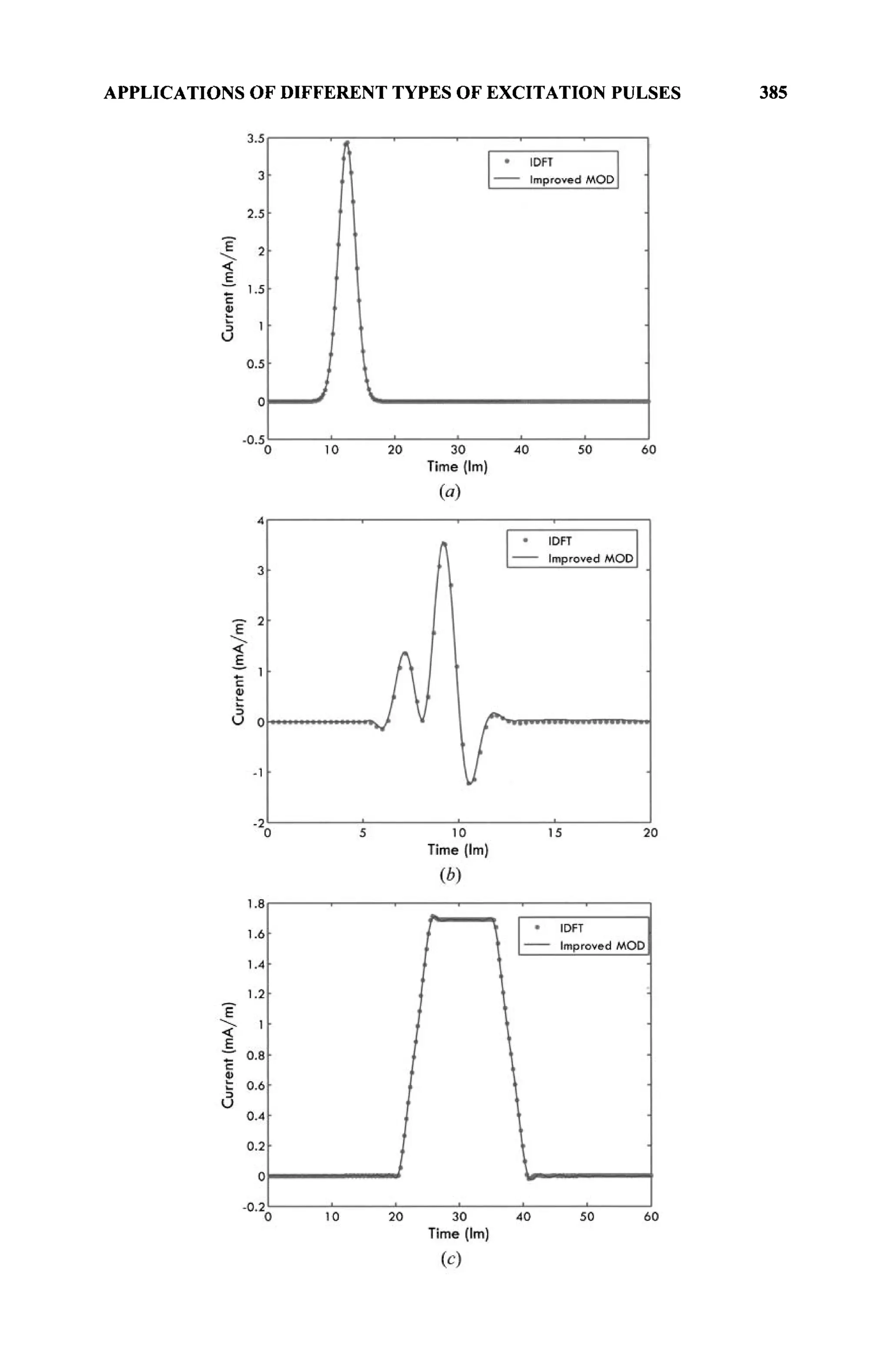
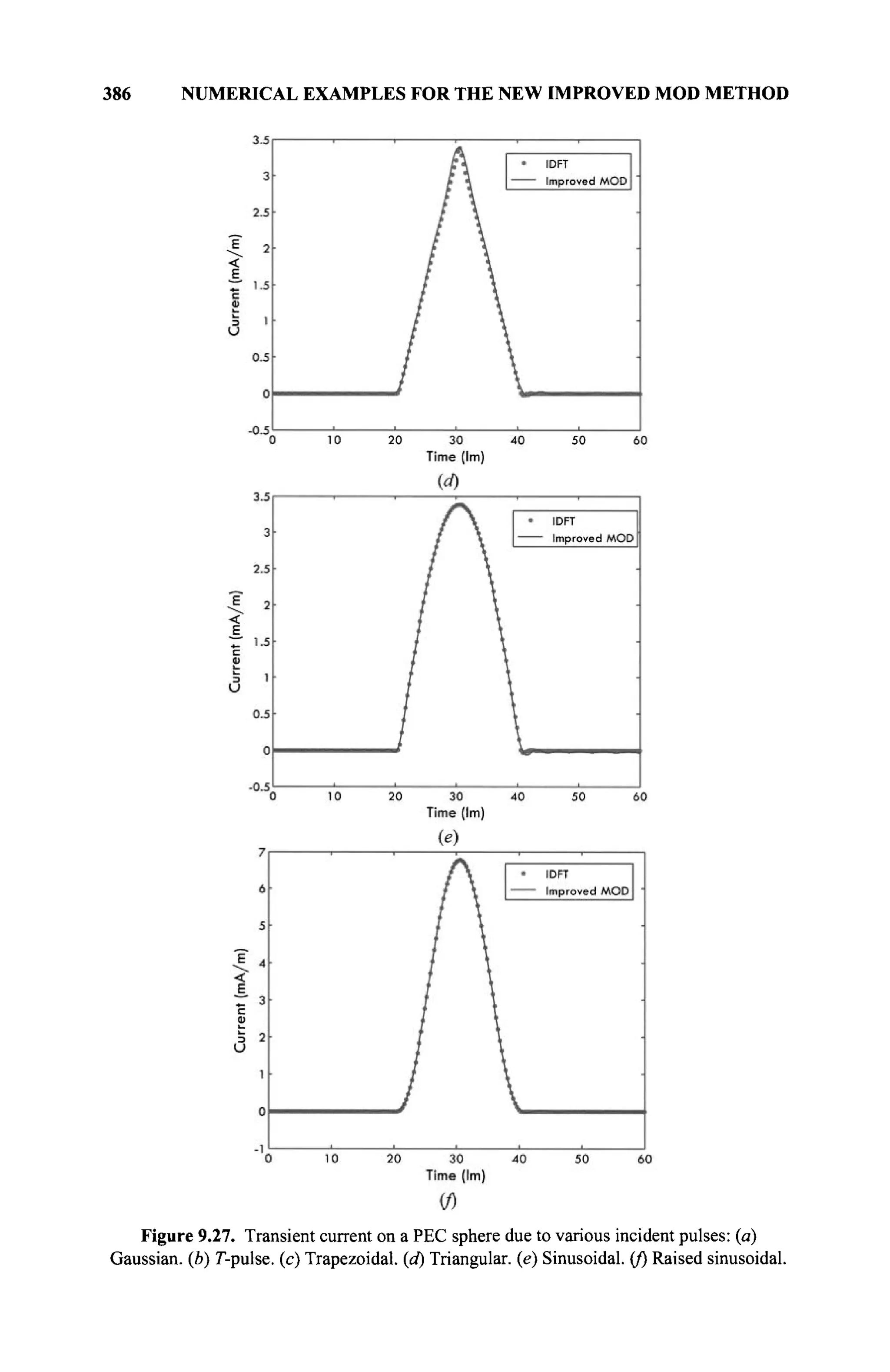
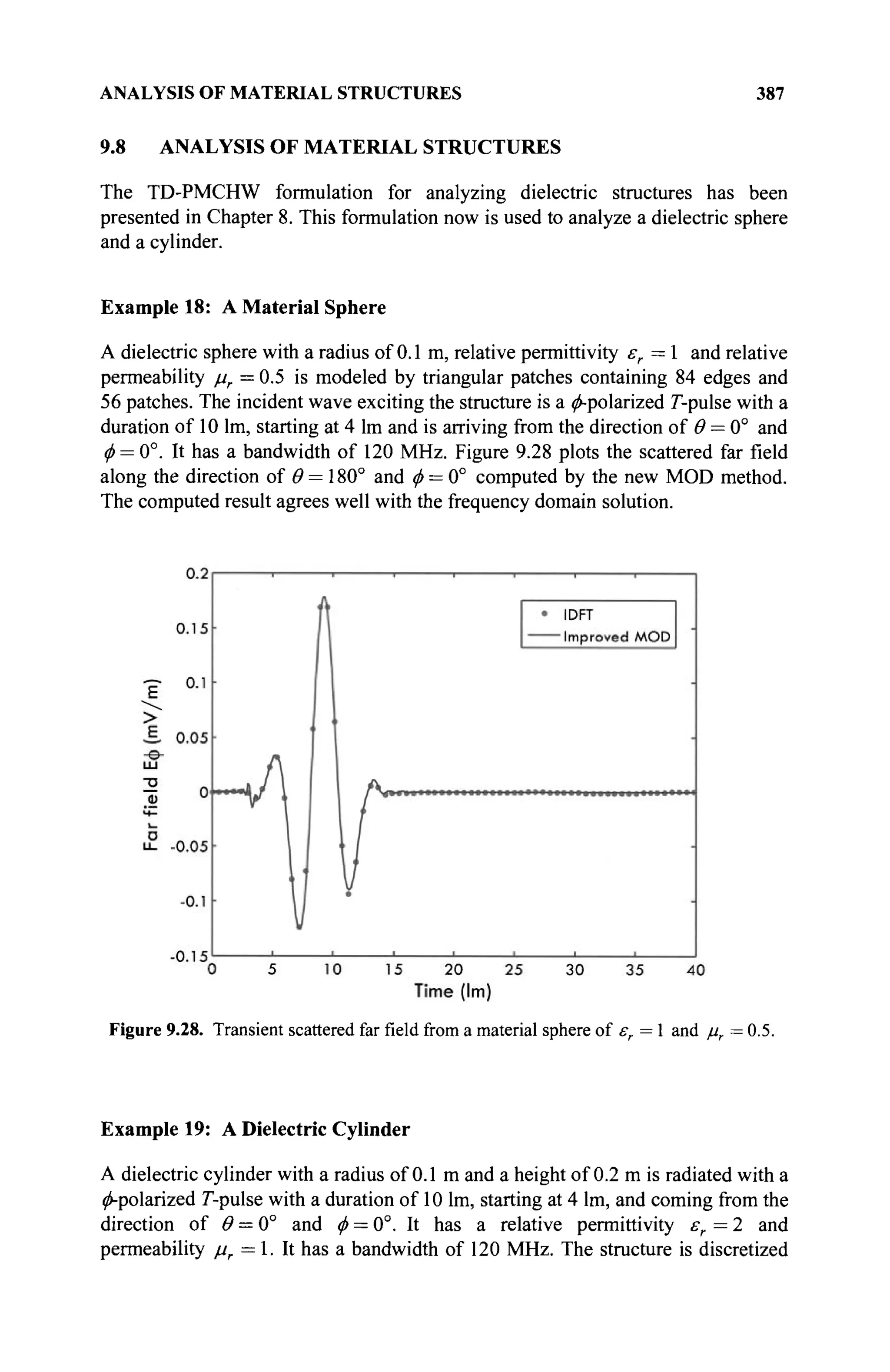
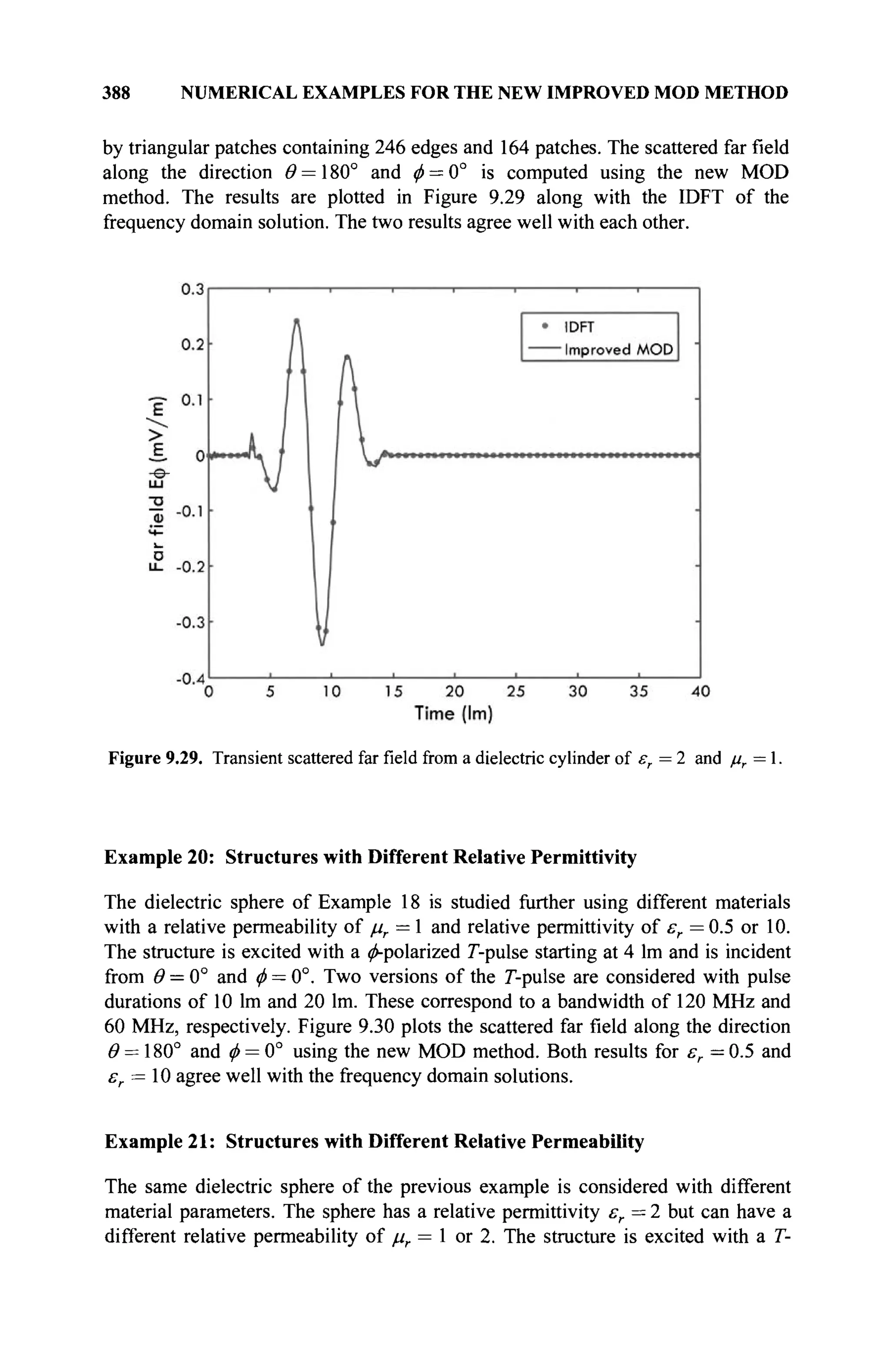
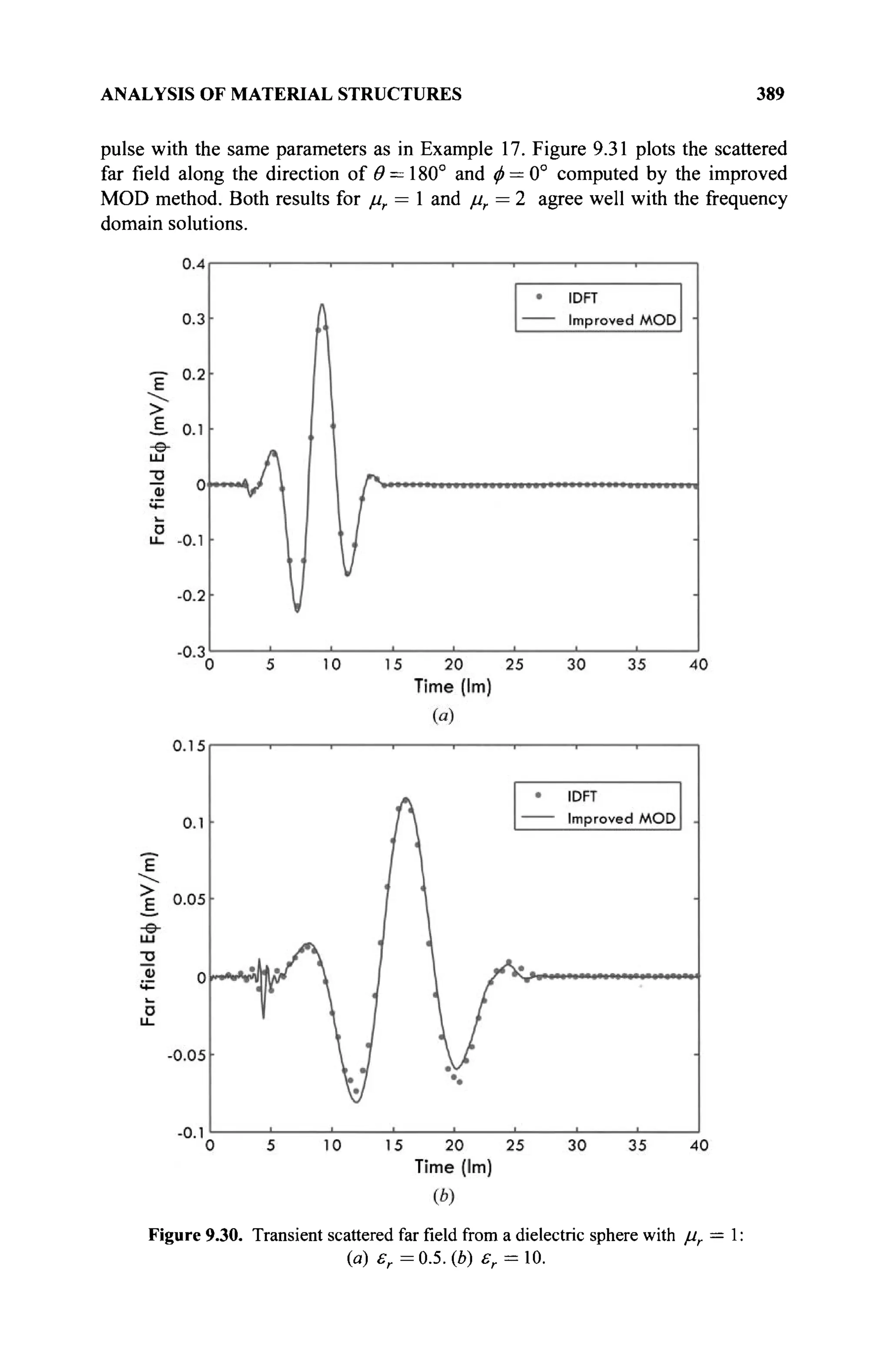
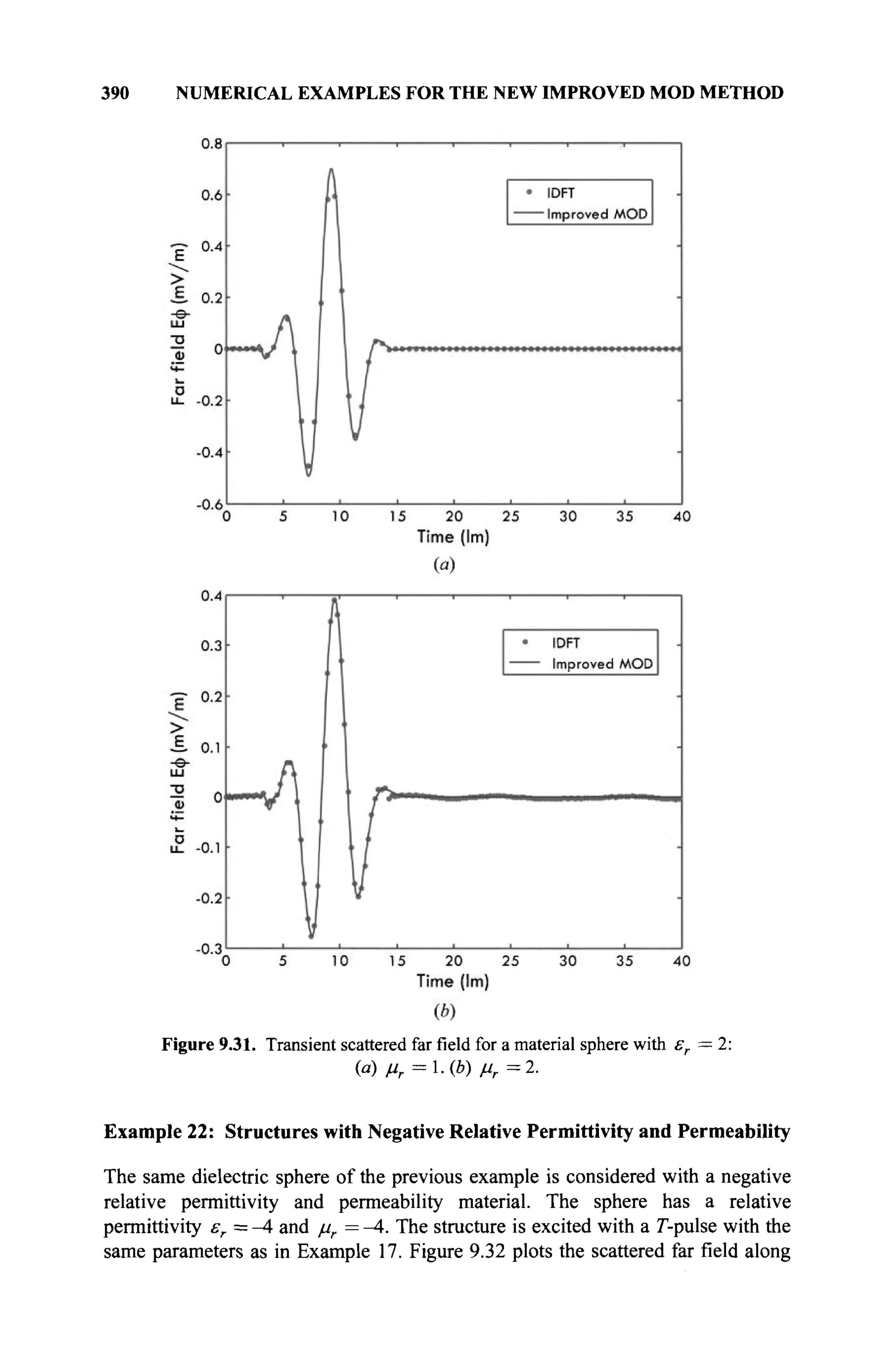
![REFERENCES 391
the direction of θ = 180° and φ = 0° computed by the improved MOD method.
The result for agrees well with the frequency domain solutions.
Figure 9.32. Transient scattered farfieldfor a material sphere with
9.9 CONCLUSION
In this chapter, the effectiveness of the new improved MOD formulations for
conducting and dielectric objects has been verified using various examples. It is
evident that the new, improved MOD method provides better stability and
efficiency than the conventional time domain MOD method. It also demonstrates
that the method can analyze a broad variety of complex conducting and dielectric
structures, both with or without loads, and material bodies with different
permittivity and permeability. The structures also can be excited using different
types of incident pulses, which do not need to be continuous.
REFERENCES
[1] Y. Hua and T. K. Sarkar, "Design of optimum discrete finite duration orthogonal
Nyquist signals," IEEE Trans, on Acoust, Speech Signal Process., Vol. 36, pp. 606-
608, 1988.
[2] T. K. Sarkar, M. Salazar-Palma, and M. C. Wicks, Wavelet Applications in
Engineering Electromagnetics, Artech House, Norwood, Mass. 2002.](https://image.slidesharecdn.com/timeandfrequencydomainsolutionsofemproblemsusingintegralequationsandahybridmethodologyb-250205130750-568a5ba2/75/Time-and-Frequency-Domain-Solutions-of-EM-Problems-Using-Integral-Equations-and-a-Hybrid-Methodology-B-H-Jung-pdf-410-2048.jpg)
![394 HYBRID METHOD USING EARLY-TIME AND LOW-FREQUENCY
in the continuous domain are presented to illustrate how the extrapolation is
carried out. This method is referred to as parametric because the performance of
the extrapolation is dependent on the choice of the parameters of the polynomials,
which include the scaling factor and the order. By analyzing the properties of the
polynomials and their transforms, the converging range of parameters can be
determined analytically a priori, and some error bounds can be defined. In addition,
an iterative method to generate the solution also is described.
The second hybrid algorithm described is nonparametric. It will be shown
that a particular realization of this iterative hybrid method is equivalent to a
Neumann-series solution of an integral equation of the second kind. It is shown
further that this iterative Neumann expansion is an error-reducing method. Hence,
this integral equation can be solved efficiently by employing a conjugate gradient
iterative scheme. The convergence of this scheme also is demonstrated. The matrix
equations that generate these methodologies are developed, and the equivalence to
the integral equations is shown. Also, the method of singular value decomposition
(SVD), used for solving the matrix equation, provides accurate and stable results.
Error bounds also are provided to assess the accuracy of this methodology.
The computational load for the electromagnetic analysis for this
method is modest compared with solving the electromagnetic analysis problem
exclusively in either time or frequency domain. Numerical examples are
presented to illustrate the principles of each of these methodologies.
10.1 INTRODUCTION
Current trends in computational electromagnetics primarily are confined to the
analysis of systems in only one domain. Either one analyzes the electromagnetic
system in the frequency domain by using the method of moments (MoM), finite
element, or finite difference techniques or solves the Maxwell equations in the
time domain using a similar set of methodologies. The strategy then of solving for
the electromagnetic response from an electrically large scatterer is to use a bigger
and faster supercomputer. Therefore, the response that one can solve for
essentially is limited by the hardware of the supercomputer. However, the desired
solution may not necessarily be ultra-wideband, but still, one may need to compute
the response from an electrically large structure. Hence, we need to look at
alternative methodologies, as the traditional tools are inadequate to address this
problem because they take a long time to generate a solution.
In electromagnetic analysis, field quantities usually are assumed to be
time harmonic. This suggests that the solution lies in the frequency domain. The
MoM, which uses an integral equation formulation, can be used to perform the
frequency domain analysis as outlined in the first four chapters. However, for
broadband analysis, this approach can get very computationally intensive, as the
MoM program [1] needs to be executed for each frequency of interest, and for
high frequencies, the size of the matrix that needs to be solved for can be very
large. So for a given computer system, how large a problem one can analyze is
dictated by the memory (both real and virtual) of the computer and assumes that
the computer system does not fail during the numerical solution of the problem of](https://image.slidesharecdn.com/timeandfrequencydomainsolutionsofemproblemsusingintegralequationsandahybridmethodologyb-250205130750-568a5ba2/75/Time-and-Frequency-Domain-Solutions-of-EM-Problems-Using-Integral-Equations-and-a-Hybrid-Methodology-B-H-Jung-pdf-412-2048.jpg)
![INTRODUCTION 395
interest. To speed up the computations in the frequency domain, Cauchy's method
[2,3] was introduced so that one could interpolate/extrapolate the response without
the need to solve the problem at each single frequency of interest. The Hubert
transform [4-6] concept also was used to attain the same goal. As opposed to
Cauchy's method, which is a model-based parametric methodology and therefore
only works adequately for conducting structures, the non-parametric Hubert
transform-based methods are more general in nature, but their applicability is
limited as to how far one can extrapolate the response. The time domain [7,8]
approach is generally the preferred technique for broadband analysis. Other
advantages of a time domain formulation include easier modeling of nonlinear and
time-varying media and use of time gating to eliminate unwanted reflections. For a
time domain integral equation formulation, the marching-on-in-time (MOT)
usually is employed to solve it. A serious drawback of this algorithm is the
occurrence of late time instabilities in the form of high-frequency oscillations. To
remove this difficulty, generally an implicit technique is proposed as outlined in
the Chapters 5 and 6. One way to reduce the numerical instability in the MOT
scheme is to use the marching-on-in-order (MOD) methodology as described in
Chapters 5-9. An ultra-wideband analysis of an electromagnetic system is limited
by the execution times and not so much by the memory as for a direct MOT/MOD
solution, a matrix inversion is required only once and not for each instances when
new results need to be generated. The time domain computational techniques have
been speeded up by using the matrix pencil method [9,10]. The matrix pencil
method approximates the late-time domain response (in an interval that occurs
after the incident pulse has passed the object) by a sum of complex exponentials
and then extrapolates the response for very late times reducing the execution time.
The problem with this methodology is to determine what exactly is late time. In
finding the response from a deep cavity, the incident pulse simply bounces back
and forth inside the structure and it is not clear when the resonances are set up,
thereby defining the late-time condition. In addition, this model of extrapolating
the electromagnetic responses by fitting the late-time domain data by a sum of
complex exponentials may not be a good approach if the data are from lossy
dielectric bodies. In that case, the extrapolation does not work as the
electromagnetic response may have a different functional model other than from a
pole singularity!
In this chapter, we present a hybrid methodology that overcomes the
limitations of solving the electromagnetic problem exclusively in one domain. The
term hybrid technique is used because we do not solve the problem exclusively
only in one domain. We use a frequency domain code and generate the
low/resonant frequency response, which requires modest computational resources.
Next, we take a time domain code and generate the early-time response from the
system, which is also easy to carry out. The claim here is that the early-time and
the low-frequency information completely determines the entire response in either
domain, as these two pieces of information are complementary. The low/resonant
frequency data provides the very late-time response, which is missing and the
early-time data provides the high-frequency response, which is not in the given
data. Therefore, this new hybrid methodology is not an extrapolation scheme as
we are not creating any new information but processing the given sets of data in](https://image.slidesharecdn.com/timeandfrequencydomainsolutionsofemproblemsusingintegralequationsandahybridmethodologyb-250205130750-568a5ba2/75/Time-and-Frequency-Domain-Solutions-of-EM-Problems-Using-Integral-Equations-and-a-Hybrid-Methodology-B-H-Jung-pdf-413-2048.jpg)
![396 HYBRID METHOD USING EARLY-TIME AND LOW-FREQUENCY
different domains, which contain all the necessary information, in an intelligent
fashion. Using early-time and low-frequency data, we obtain stable late-time and
broadband information. The overall analysis is thus computationally very efficient.
The time and frequency domain responses of three-dimensional (3D)
material bodies are considered in this chapter. It is assumed that a band-limited
ultra-wideband pulse excites the material body. The band-limited assumption is
not only necessary but also mandatory. The reason for this is that for numerical
analysis we need to discretize the structure spatially. To obtain accurate results,
the triangular patches modeling the surface of the material body should be at least
a tenth of a wavelength (the wavelength is defined in terms of the path length
inside the material body) at the highest frequency of interest or smaller. Otherwise,
there would be aliasing errors in the response. This spatial discretization of the
material body puts a hard limit on the highest frequency that can excite the
structure. Therefore, the frequency domain response is strictly band limited and let
this be 25, as the response in frequency stretches from —B to +B. However, that
bandwidth В could be very large. On the other hand, the time domain response is
not strictly limited in time, but for practical reasons, in a numerical experiment, we
want to extrapolate the response up to some time Го, such that both the time and
frequency domain responses are of finite support for all practical purposes. Two
methods are described in this chapter to carry out this extrapolation procedure.
They are termed parametric and nonparametric.
The first hybrid algorithm introduced in this chapter in section 10.2 is
parametric [11-17]. An orthogonal series along with its Fourier transform using
the same unknown coefficients linearly combining the various functions is used to
fit the data both in the time and frequency domain. One then solves for these
unknown coefficients by matching the various polynomials and its transforms
using early-time and low-frequency data. These coefficients then are used to
extrapolate the response both for late-time and high-frequency. Orthogonal
functions based on the three polynomials (namely the Hermite, Bessel-Chebyshev,
and Laguerre) in the continuous domain have been presented to achieve this goal
of extrapolation [15,16]. The hybrid method in the discrete domain using a
discrete Laguerre polynomial has been introduced in Ref. [17]. Fourier Transforms
of the presented polynomials are analytic functions. This allows work to be
performed simultaneously with time and frequency domain data. This method is
referred to as parametric because the performance of the extrapolation is
dependent on the choice of the scaling factor and the order of the polynomials. By
analyzing the properties of the polynomials and their transforms the region of
convergence of the parameters can be determined analytically a priori [15] and
some error bounds can be defined. In addition an iterative method to generate the
solution also is described.
The second hybrid algorithm described in section 10.3 is nonparametric
[18]. This implies that no parameters are optimized to get the appropriate solution.
The total solution, however is calculated based on the physics of the problem. It
will be shown that a particular realization of this iterative hybrid method is
equivalent to a Neumann-series solution of an integral equation of the second kind.
It also is shown that this iterative Neumann expansion is an error-reducing method.
This integral equation can be solved efficiently by employing a conjugate gradient](https://image.slidesharecdn.com/timeandfrequencydomainsolutionsofemproblemsusingintegralequationsandahybridmethodologyb-250205130750-568a5ba2/75/Time-and-Frequency-Domain-Solutions-of-EM-Problems-Using-Integral-Equations-and-a-Hybrid-Methodology-B-H-Jung-pdf-414-2048.jpg)
![A PARAMETRIC HYBRID SOLUTION METHODOLOGY 397
iterative scheme. The convergence of this scheme also is demonstrated. The matrix
equations that generate these methodologies are developed and the equivalence to
the integral equations is shown. Also, the method of singular value decomposition
(SVD) [19], used for solving the matrix equation, provides accurate and stable
results. Error bounds also are provided to assess the accuracy of this methodology.
Computational load for the electromagnetic analysis for this hybrid
method using either the parametric or the nonparametric methodology is modest
compared with solving the electromagnetic analysis problem exclusively in either
time or frequency domain. Numerical examples are presented to illustrate the
principles of each of these methodologies. Section 10.4 provides some conclusions
followed by some selected references where additional materials can be obtained.
10.2 A PARAMETRIC HYBRID SOLUTION METHODOLOGY
The objective is to generate a broadband electromagnetic (EM) response at various
spatial locations on the structures of interest in either time or in the frequency
domain. This broadband response is generated using a time-frequency hybrid
methodology. This hybrid methodology is a combination of the data generated
using early-time and low-frequency information. In summary, we are fitting a
given data set along with its transform using a set of orthogonal polynomials along
with their transforms containing the same coefficients. Because we fit the data in
these two complementary domains by using a set of orthogonal polynomials along
with their respective transforms, it is termed a parametric hybrid solution
methodology. The philosophy here is that the given data in both the domains time
and frequency, will be parameterized by some known quantities with some
unknown constants. The various orthogonal polynomials and how they can be
used effectively along with the error estimates involved in the approximation are
discussed next.
The early-time response generated by a time domain code provides Ml
samples with the sampling step of At. This time domain data set is designated by
x,. The low-frequency response at the same spatial location is evaluated at M2
points with the sampling step of A/. This frequency domain data set is designated
by X[. The missing late-time and high-frequency data sets are similarly designated
by x2 and X2, respectively. The complete time and frequency domain responses
are given by the functions x(t) and X(f), respectively. The total number of
samples that characterize x(t) is Mh and the total number of samples that
characterize X{f) is Mf. These relationships are given by](https://image.slidesharecdn.com/timeandfrequencydomainsolutionsofemproblemsusingintegralequationsandahybridmethodologyb-250205130750-568a5ba2/75/Time-and-Frequency-Domain-Solutions-of-EM-Problems-Using-Integral-Equations-and-a-Hybrid-Methodology-B-H-Jung-pdf-415-2048.jpg)
![398 HYBRID METHOD USING EARLY-TIME AND LOW-FREQUENCY
*1 = {*('о)>*('1)>"-»*('л/,-1)}
x
2 = {х0м1)>х(*М1+)>->х
(*м,-1)}
Xl = {X(f0),X(fl),...,X(fM2.])f
Χ2={Χ(/Μ2ΙΧ(/Μ2+Ι),-,Χ(/Μ/-1)}Γ
(10.1)
In Eq. (10.1), tj=(i — l)At and f-=(j — l)Af. The complete data set then is
characterized by concatenating the given and the missing data sets as
x = X = (10.2)
The basic philosophy of the parametric hybrid method is to fit x(t) and X(f) by
a series of orthogonal polynomials and their transforms, respectively, using the
same parameters. Suppose the time domain response is fitted by the expression
x{t) = Y,aMt'h) = Σ«Λ('>4) (10.3)
n=0 л=0
where φη(ί) is the orthogonal basis function of degree n and is a scaling
factor. The objective of the scaling factor is to scale the axis of the data, be it in
picoseconds, microseconds, and so on. Therefore, the frequency domain response
automatically is fitted with the transform of Eq. (10.3) as
л=0 я=0
(10.4)
where фп (t) and Фп (/) are related by the Fourier transform and the two scaling
factors /j and /2 are related by
/2 =l/(2*/,) (10.5)
To solve for the unknown coefficients a„, only the early-time and the low-
frequency information is used. For a numerical solution of the coefficients a„, the
infinite upper limit in Eqs. (10.3) and (10.4) are replaced by a finite number ./V
resulting in the following matrix equation:](https://image.slidesharecdn.com/timeandfrequencydomainsolutionsofemproblemsusingintegralequationsandahybridmethodologyb-250205130750-568a5ba2/75/Time-and-Frequency-Domain-Solutions-of-EM-Problems-Using-Integral-Equations-and-a-Hybrid-Methodology-B-H-Jung-pdf-416-2048.jpg)
![A PARAMETRIC HYBRID SOLUTION METHODOLOGY 399
Re
Im
Фо^м^Л) Ф('мх-А)
Α ( / ο Λ ) <Ρι(/ο./2)
*ο(/ι./2) <Ρι(/ι,/2)
[Φο(ίο^) ΦΛ/oJi)
Φ0(/,Λ) <Pi(/i,/2)
Φο(Λί2-ι./2) <Ρι(Λί2-ι.'2)
^v-iiWi)
$ν-ι(Ί>Ί)
^Λ'-ιί'Ά/,-ιΆ)
<Pjv-i(/o>'2)
<Ρ*-ι(/ι.ί2)
ΦΝΜΜ2-ΊΙ),
ΦΝ-ΑίΜ
ΦΝΜΜ
ΦΝΜΜ,^Ι)
Re
Im
JC(/0)
χ(Γ,)
ί*(/ο)
Α-(/,)
*(Λ,2_,)
И/о) '
X(fù
XUu2-x)
(10.6)
where Re(·) and Im(·) stands for the real and imaginary parts of the transfer
function. Then, once the N coefficients {«„}, have been solved for, they can be
used in Eq. (10.3) to extrapolate the late-time response and in Eq. (10.4) to
extrapolate the missing high-frequency response. The values x2 and X2 are
designated as the corresponding extrapolated data, (i.e., the estimation for x2 and
X2 ). Eq. (10.6) shows that N<Ml + 2M2. The question now is how many
functions T
V are required in Eqs. (10.3) and (10.4) instead of oo.
It is assumed that the response that we are interested in is strictly band-
limited up to a frequency B. This is justified, as explained before, because one
needs to discretize the structure spatially for computational reasons. Typically, one
uses about 10 expansion functions per wavelength in the material body (of course
this depends on the numerical method; a value of 10 is chosen for illustrative
purposes), and therefore, the spatial discretization of the structure limits the high-
frequency response (and let us say it is up to B). If we now are interested in
representing the same waveform in the time domain, then it is of infinite duration.
However, for a numerical method, we cannot go to infinity and the record is
assumed to be limited to a time of duration T0. Then the question is how many
parameters are necessary to represent mathematically that waveform, which is also
band limited by В (the frequency goes from -B to +B). We now demonstrate that
(22?7o + 1) pieces of information are sufficient to describe that waveform from a
strictly mathematical point of view. To prove this, we represent the real-time
domain function x(t) by a Fourier series. This is permissible because the waveform
is strictly band limited, so that [20,21] x(i) = ^ C p exp(ipco0t) where ω0=—.
P T
0
Because x(t) is real, С = С where * represents the complex conjugate. If x(t) is
band limited to В Hz, then the range of the summation index p is fixed by -B <pf0](https://image.slidesharecdn.com/timeandfrequencydomainsolutionsofemproblemsusingintegralequationsandahybridmethodologyb-250205130750-568a5ba2/75/Time-and-Frequency-Domain-Solutions-of-EM-Problems-Using-Integral-Equations-and-a-Hybrid-Methodology-B-H-Jung-pdf-417-2048.jpg)
![400 HYBRID METHOD USING EARLY-TIME AND LOW-FREQUENCY
ВТ
< В, and becausef0 = 1/T0, we obtain x(t)= ^ С exp(ipw01). Hence, there
P=-BT0
are exactly 2BT0 + 1 terms in this expansion of x{t). Therefore, the dimensionality
N in Eq. (10.6) reflects 7^= 2BT0 + 1. From a strictly mathematical standpoint, one
needs a total of 2BT0+l samples to characterize the ultra-wideband waveform of
bandwidth 2B and of time duration T0. These 2BT0 + 1 samples can be entirely in
the time domain or in the frequency domain or a combination, being partially in of
both the domains. These samples are then sufficient from a strict mathematical
perspective to represent any waveform. However, from a numerical perspective, if
these samples are too close to each other, then the solution of Eq. (10.6) would be
very ill conditioned and the extrapolation may fail. One way to know whether the
samples are spaced adequately and whether their numbers are adequate from a
strictly numerical perspective (even though it may be sufficient from a strictly
mathematical point of view) is to carry out a total least-squares solution [2,19] of
Eq. (10.6) instead of using an iterative method such as the conjugate gradient to
solve for the coefficients. The distribution of the singular values in the total least-
squares solution [2,19] will provide an automatic methodology to know whether
the data lengths are adequate. This point will be illustrated later on. We find that
taking samples simultaneously in both domains provides a much more stable
solution than just taking them in one domain exclusively. Therefore, we must have
the total number of samples Mj in the time and M2 in frequency equal to M +M2 >
N=2BT0+l.
Finally, what is the optimum sampling rate in time and frequency is still
an open question.
To evaluate the performance of this hybrid method, the following
normalized mean-squared errors (MSE) are used in the time and frequency domain
as
II » II V Y
_ II x
2 *21|2 p _ II 2 2
lb n o 74
' ~ ~hT— f
~ " 1 x 1 —
II x
2 lb IIA
2 lb
where || · || is the З'г norm of a vector. If x2 and X2 are equal to 0 (trivial
results), then Et and Ej- will be equal to 1. Therefore, the hybrid method does not
converge when Et > 1 or Ej>. The goal of this section is to demonstrate
through numerical examples that it is possible to carry out such a hybrid solution
with good accuracy. In this way, the computational time can be reduced
significantly.
The success of this procedure depends on the choices of the parameters
Δ/, Af, Mx, M2, l, /2,and N. The choice of At and Af is restricted by the
Nyquist's theory of sampling, which states that Δί>ΐ/(2^) andA/>l/7 The
variables T and W discussed in this chapter are the time support and the
bandwidth for the electromagnetic responses x(t) and X(f), respectively. For
the choice of Mx and M2, it is clear that {Mx + 2M2) should be greater than N,
whatever that value is.](https://image.slidesharecdn.com/timeandfrequencydomainsolutionsofemproblemsusingintegralequationsandahybridmethodologyb-250205130750-568a5ba2/75/Time-and-Frequency-Domain-Solutions-of-EM-Problems-Using-Integral-Equations-and-a-Hybrid-Methodology-B-H-Jung-pdf-418-2048.jpg)
![A PARAMETRIC HYBRID SOLUTION METHODOLOGY 401
Notice that the matrix of Eq. (10.6) need not be a square matrix, and it
may be ill-conditioned if the time and frequency samples of the response are close
to each other. That is why we advocate the use of the singular value decomposition
(SVD) method [19] to solve Eq. (10.6). There are two reasons of doing that. First,
it can tell us whether we have sufficient data to begin with in both the domains to
carry out the extrapolation in the two domains, and second, even if the data sets
given are sampled closely, it does not influence the final result, as the SVD still
can provide a solution for {an} in a least-square sense. Hence, the solution, when
it exists, has a minimum norm for x2 and X2. This feature is in accordance with
the assumption that the early-time data complements the high-frequency
information and the low-frequency data complements the late-time information.
Another advantage of using SVD is that the distribution of the singular values can
be analyzed. SVD will "provide an automatic methodology to know whether the
data lengths are adequate" [10]. A tolerance {toi) of the singular values can be
chosen to be of the same level as the numerical error and the noise of the original
data. If the smallest singular value of the matrix is larger than the toi, it means Mx
or M2 is not large enough, and the time domain or the frequency domain codes
has to be executed to obtain more data and the extrapolation cannot proceed.
However, when the value of the smallest singular value is less than the value of
toi, which implies that that there is sufficient data and a solution can be obtained.
In computing that solution using the singular vectors, the information related to the
singular values smaller than toi is discarded. Therefore, in this procedure, what is
early-time and low-frequency is not defined clearly. However, using Mx and M2
samples of the data, along with the SVD, one can determine a priori whether the
data sets given are sufficient or not. If the data sets are not sufficient by observing
the magnitude of the various singular values, then additional data must be
generated in either domain.
Next, we choose the value of N, which is required to approximate any
time-domain function of duration T and bandwidth 2W and is determined by the
time-bandwidth product of the signal or by the dimensionality theorem, also called
the 2NW theorem [20,21]. It is also a different statement for the sampling
theorem. Consider a Fourier transform pair
h(t)^H(f) (10.8)
and # ( / ) is approximately band-limited and so |/| < W. The energy outside W
is small and has an upper bound of ε.
fH(f)2
df<£
f>w
Consider G to be the set of finite energy sequences. In addition, h and M is the
dimension of the smallest linear space of sequences that approximate G on the](https://image.slidesharecdn.com/timeandfrequencydomainsolutionsofemproblemsusingintegralequationsandahybridmethodologyb-250205130750-568a5ba2/75/Time-and-Frequency-Domain-Solutions-of-EM-Problems-Using-Integral-Equations-and-a-Hybrid-Methodology-B-H-Jung-pdf-419-2048.jpg)
![402 HYBRID METHOD USING EARLY-TIME AND LOW-FREQUENCY
index set (0, N — Ï), with energy less than ε', and N is the number of time
samples or the dimension of G. Then
N-
Σ
и=0
M
Sn-J2a
jSn
7=1
U) <ε' (10.10)
where gn is a sequence such that {g} e G and a, are the coefficients of
approximation. Then, the 2NW theorem can be stated as follows: For
1/2 > W > 0 , the sampling time needs to be less than the Nyquist sampling
interval, and when ε' > ε > 0, we obtain
lim — = 2W (10.11)
The fact can be summarized succinctly as follows: For a large value of N, the set
of sequences of bandwidth W that are confined to an index set of length about M
has dimensions approximately equal to the time-bandwidth product of the
waveform, which is equal to 2NW. Here, the sampling interval in time domain is
assumed to be unity. If AT is the sampling interval in time domain, then the order
or the degrees of freedom of the expansion is approximately 2NWAT, as stated
by the sampling theorem.
In summary, as long as the total number of the orthonormal basis
functions exceeds the time-bandwidth product of the EM response, they are
sufficient to approximate any function in the ^-norm. The choice of the values
of the remaining parameters, /, and l2,is a little involved, as it depends on the
type of orthogonal polynomial chosen to approximate the functions. Also, note
that it is necessary to choose only one of the scaling factors, as the scaling factor in
one domain is related to the other through Eq. (10.5). It is important to note that
the expansion given by Eqs. (10.3) and (10.4) only converge for certain values of
the parameters and not for all values. Therefore, it is important to reflect on how to
arrive at the optimum values of these parameters. Ref. [22] seeks the optimal value
for lx analytically in synthesis of systems using Laguerre polynomials. The
optimal scaling factor should be one of the roots of the following equations:
cL(b) = 0
cL+l(b) = 0
(10.12)
(10.13)
where b is a value relative to the scaling factor and cL (b) is a polynomial given
by
. N min(/',L)
cL(b) = ^bI
j2 Σ (-DL
L — s + i
i
а,Ь(i+L-2s)
(10.14)](https://image.slidesharecdn.com/timeandfrequencydomainsolutionsofemproblemsusingintegralequationsandahybridmethodologyb-250205130750-568a5ba2/75/Time-and-Frequency-Domain-Solutions-of-EM-Problems-Using-Integral-Equations-and-a-Hybrid-Methodology-B-H-Jung-pdf-420-2048.jpg)
![406 HYBRID METHOD USING EARLY-TIME AND LOW-FREQUENCY
10,2.1.2.1. Hermite Basis Functions. First, choose the orthogonal basis function as
<p„(t,ll) = h„(t,ll) where h„(t,lx) are the associated Hermite polynomials. They
can be expressed as
H
KM
t
[A)
4Тп~ /1Л/7Г
(10.19)
, л = 0,1, 2,...
where Hn(t) is the Hermite polynomial. The Hermite polynomial can be
computed recursively through [23]
H0(t) = l, #,(0 = 2/ (10.20)
H„{t) = 2/Яи _,(0-2(«-1)Яя „2 (0; п = 2,3,4,...
Thus the associated Hermite polynomials are calculated recursively by
Ηη{ί) = ^=(42ί hn_x{t)-4n~^hn_2{t), « = 2,3,4,... (10.21)
V«
Because the associated Hermite polynomials are the eigenfunctions of the Fourier
transform operator, their Fourier transforms are given by
hn{t, /,) â hn{tllx) ^ (-if hn(fll2) â (-/)"*„(/, /2) (10.22)
So, if the function x(t) can be expanded by the orthogonal basis «„ (t, l{ ), its
Fourier transform X(f) can be obtained by adding up the terms
{-i)"hn(f, /2) with the same coefficients. It is observed that the associated
Hermite polynomials are not necessarily causal, and in addition, its two properties
in the time domain are:
1. The time support of the basis function Tn increases as the order n
increases, assuming the scaling factor /, is fixed. This property is because
of the following relation:
l i m - ^ - = 0; « = 0,1,... (10.23)
<-oo«„+1(0
2. More oscillations occur for the functions as the order « increases.
Because of Eqs. (10.22) and (10.23), it can be observed that the basis
function with a higher order has more high frequency components.](https://image.slidesharecdn.com/timeandfrequencydomainsolutionsofemproblemsusingintegralequationsandahybridmethodologyb-250205130750-568a5ba2/75/Time-and-Frequency-Domain-Solutions-of-EM-Problems-Using-Integral-Equations-and-a-Hybrid-Methodology-B-H-Jung-pdf-424-2048.jpg)
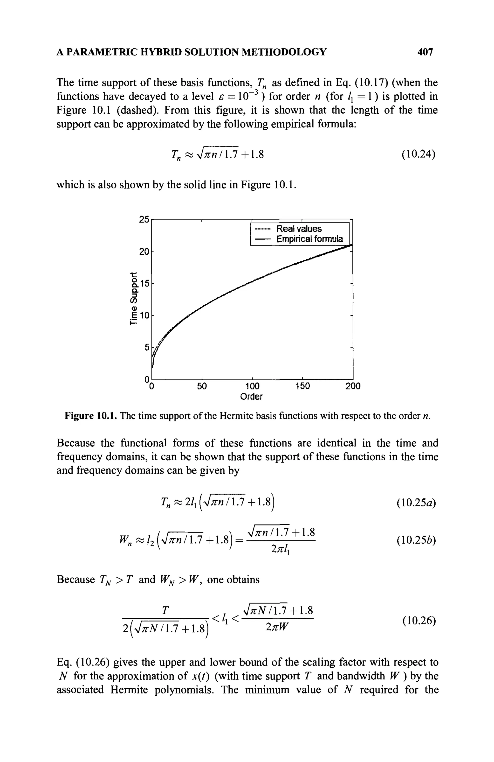
![408 HYBRID METHOD USING EARLY-TIME AND LOW-FREQUENCY
extrapolation is relative to WT. Because only two conditions are considered,
TN>T and WN >W, the implicit lower bound of N in Eq. (10.26) is more
relaxed than the value given by the "2WT theorem" [20,21]. The 2WT theorem
states that the "approximate dimension of the signal" is N = 2WT, resulting in a
lower bound on N as
N>2WT (10.27)
Eq. (10.27) is used as the lower bound for N when employing the Hermite basis
functions. Although N has a lower bound only, it cannot be arbitrarily large
because the magnitude of the coefficients an will have oscillations for large
values of N because of computational error.
10.2.1.2.2. Bessel-Chebyshev Functions. Another choice for the orthogonal basis
function is<pn(t,lx) = (t/ll)~i
Jn[t/l]) where ./„(///,) is a Bessel function of the
first kind of degree n. A waveform with a compact time support can be expanded
as
χ(/)»£;α|Ι(///,Γ,
Λ('/Α)Ε
Σα
»(///
ιΓ1
Λ(ί.Α)
и=0 л=0
The Fourier transform of Eq. (10.28) can be evaluated as [15]
(10.28)
X{f)-
N
,2l>^.
Σ«--Η)"ι-(//'2Γ2
^-.(//'2);|/|<'2
„=0 n L J
0 >f>h
(10.29)
where l2 = 1/(2πΙ{) and U„(f) is the Chebyshev polynomial of the second kind
defined by [23]
un(fY
sin[(« + l)cos / ]
( i - / 2
) X
(10.30)
In Eqs. (10.28) and (10.29), the causality in time is not forced, whereas the
waveforms being used are causal. The relationship between the first and second
kind of Chebyshev polynomials is given by the Hubert transform that is,
j-fZ^w^^w
y-x
(10.31)
where T£(x) is the Chebyshev polynomial of the first kind defined by](https://image.slidesharecdn.com/timeandfrequencydomainsolutionsofemproblemsusingintegralequationsandahybridmethodologyb-250205130750-568a5ba2/75/Time-and-Frequency-Domain-Solutions-of-EM-Problems-Using-Integral-Equations-and-a-Hybrid-Methodology-B-H-Jung-pdf-426-2048.jpg)
![A PARAMETRIC HYBRID SOLUTION METHODOLOGY 409
r„c
(/) = cos[/icos-,
(/) (10.32)
Therefore, a causal time domain waveform and its Fourier transform can be
written as
N
Φ ) = ! > „ ( / / / , ) ■/„(///,);*><> (10.33)
* ( / ) =
N_
= 0
0;
X
A
u,n-
I I ■; f<h
>f>h
(10.34)
Unlike the associated Hermite functions, which have the same form in time and
frequency domains with the decay rate of e~* n
or e~^ /2
for large t or f, the
Bessel-Chebyshev basis functions are strictly band limited, (i.e., |/| < /2 ). The
fact that they are strictly band limited results in infinite time support, or Tn —
► oo.
The time decay rate l/t of the functions as in Eq. (10.33) is not sufficient to make
the basis functions limited in time.
The upper bound of /] is determined from the bandwidth of the functions
obtained from the condition WN > W. Because Wn —12 for all n,
/, <Ι{2πΨ) (10.35)
Because, Tn —
► oo , the lower bound of /, cannot be decided simply by the
condition TN > T. The second criterion then is used as stated in the beginning of
this section. Bessel functions have the following asymptotic forms:
·/„(')<
1
Ди + 1)
(//2)", t «
Jn{t)?i^2l{Kt)cos(t-nKl2-KlA), t »
(10.36)
(10.37)
For large values of ? (t » 1), Jn (t) approximates a sinusoidal function with an
attenuation 1/V?. Jn (t) displays a delayed peak with an oscillating tail with the
same frequency ω = 1 for each n. This oscillation is strictly band limited by ω = 1
( /2 = 1/2л" if /] = 1 ) in the frequency domain. The tails of the basis cannot be
used to approximate an arbitrary function because all tails have only a single
frequency component. Mathematically speaking, the dimension of the set
{J„(t)n = 0, 1, 2, ..., N} is limited and cannot form a complete basis set for
t » 1, if N is not large enough. We calculate the effective time support Γ' as the](https://image.slidesharecdn.com/timeandfrequencydomainsolutionsofemproblemsusingintegralequationsandahybridmethodologyb-250205130750-568a5ba2/75/Time-and-Frequency-Domain-Solutions-of-EM-Problems-Using-Integral-Equations-and-a-Hybrid-Methodology-B-H-Jung-pdf-427-2048.jpg)
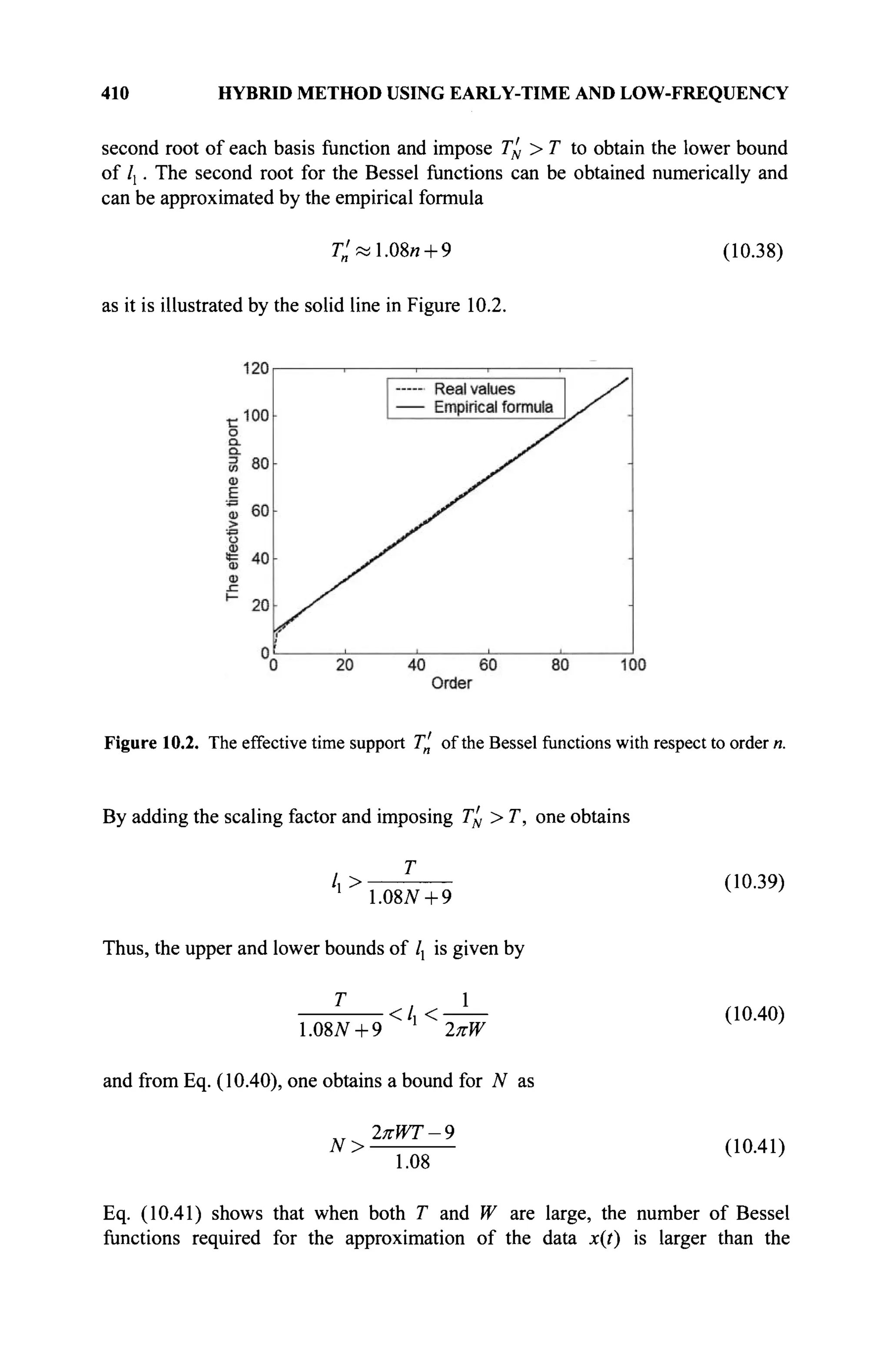
![412 HYBRID METHOD USING EARLY-TIME AND LOW-FREQUENCY
The Fourier transform of Eq. (10.47) can be evaluated as [22]
A a„ (-0.5 + j fll2)"
Μ*Σ Λ ' . , * η + 1 (10.48)
η=ο^2π12 [0.5 +jf/l2)
where l2 = /{2πΙγ ). The time support for these functions can be approximated by
T„ (when the functions have decayed to a level ε = 10~~3
) as
Г„=4.1и + 25 (10.49)
This is a good approximation, as shown by the dotted line in Figure 10.3.
Figure 10.3. The time support of the associated Laguerre functions with respect to order n.
When TN > T, the lower bound for /, is given by
/,> (10.50)
1
4.LV + 25
The Fourier transform of the Laguerre functions has a rational form in the
frequency domain as
0n(f,l2) = A{f)ei[a(f)
-"l2)
, where (10.51)
a ( / ) = (2n + l)tan-1
(/2 /(2/)) (10.52)](https://image.slidesharecdn.com/timeandfrequencydomainsolutionsofemproblemsusingintegralequationsandahybridmethodologyb-250205130750-568a5ba2/75/Time-and-Frequency-Domain-Solutions-of-EM-Problems-Using-Integral-Equations-and-a-Hybrid-Methodology-B-H-Jung-pdf-430-2048.jpg)
![A PARAMETRIC HYBRID SOLUTION METHODOLOGY 413
The amplitude of Φη{/,12) is independent of n. Now we use the second criterion
to obtain the upper bound of /], which is given by
da{f)
df f=w
>Ca (10.54)
This results in
(2N + l)2l2_ 4M2 ? c
4W2
+l2
2
~4W2
+l2
2 W (10.55)
By solving the inequality in Eq. (10.55), one obtains
/ , < ■
Cu
^IN-<JN2
-W2
C, 2 ^ 2
w
(10.56)
Together with Eq. (10.50), the upper and lower bounds of lx is given by
T , Cw
</, <
4.LV + 25 4^N-JN2
-W2
CW
2 (10.57)
and the lower bound of the number of basis functions can be found easily from Eq.
(10.57) as
'~~^ ~ (10.58)
N>.2<Jw2
Tcl, + 6-3
10.2.1.2.4. Summary. Properties of all three basis functions are summarized in
Table 10.1. The upper and lower bounds for /, along with the lower bound of N
also are given in Table 10.1. Given an EM response with a time support T and
one-sided bandwidth W, and for a fixed number N of these basis functions, the
Laguerre basis functions have the widest range of lx for an accurate
approximation of the desired response. The Bessel-Chebyshev basis functions
have the narrowest range of /,. From the bounds on /b the lower bounds on N
(except for Hermite functions) can be obtained, which also are shown in Table
10.1. Because the lower bound of Ιλ is determined by the properties of the basis
functions in the time domain, and the upper bound of lx is determined from the
properties in the frequency domain, the optimal scaling factor is expected to be
somewhere in the middle of the two bounds.
An approximate value can be obtained from the point where the lower
and upper bounds are equal. In this case, it is easier to obtain the optimal scaling
factor for the Bessel-Chebyshev functions, simply as /2πΨ, which is its upper
bounds.](https://image.slidesharecdn.com/timeandfrequencydomainsolutionsofemproblemsusingintegralequationsandahybridmethodologyb-250205130750-568a5ba2/75/Time-and-Frequency-Domain-Solutions-of-EM-Problems-Using-Integral-Equations-and-a-Hybrid-Methodology-B-H-Jung-pdf-431-2048.jpg)
![414 HYBRID METHOD USING EARLY-TIME AND LOW-FREQUENCY
The bounds shown in Table 10.1 now are validated through numerical examples
presented in the next section.
Table 10.1 The basis functions and the bounds for /,
Hermite Basis functions
Bounds for /i
Bounds for N
л/я-ЛГ/1.7+1.8
2 (V/riV/1.7+1.8)
N > 2WT
< /, <
2πΨ
Bessel- Basis functions
Chebyshev
ΦΜ) = {t/ilyl
j„(t,il)
<W,'2) = -
-{/ιι2)ψυη_γ{/ιι2
+ тп
с
{//12
Bounds for /
Bounds for N
T , 1
1.08JV + 9 2πΨ
2πΨΤ-9
N>-
1.08
Laguerre Basis functions
Φη(ί,ι]) = (ι/^)β~/2
4„{ί/ιι
H "
■Jfih
Bounds for /i
Bounds for N
-^2π12
<lx<-
+ jf'h
Cix
я+1
4.LV + 25 4„[N-JN*-W2
C
N> 1.2 JW2
TC^+ 6-3
10.2.1.3 Numerical Examples.
Example 1. In this example, a microstrip band-pass filter is chosen as the structure
of interest. It is shown in Figure 10.4. We want to obtain its broadband response](https://image.slidesharecdn.com/timeandfrequencydomainsolutionsofemproblemsusingintegralequationsandahybridmethodologyb-250205130750-568a5ba2/75/Time-and-Frequency-Domain-Solutions-of-EM-Problems-Using-Integral-Equations-and-a-Hybrid-Methodology-B-H-Jung-pdf-432-2048.jpg)
![A PARAMETRIC HYBRID SOLUTION METHODOLOGY 415
by using early time and low frequency data for the S-parameter. The microstrip
band-pass filter is designed at a center frequency of 4.0 GHz with an 8%
bandwidth and is fabricated on a substrate with relative dielectric constant of 3.38.
The height of the substrate is 1.5 mm. The other relevant dimensions of the filter
are L, = 14.5 mm, L2/L, = 1.3, Zg/L, = 1.16, W3 =20 mm, W2/Wl = 1.15, and
Gapx/Gap2 = 3.2.
Figure 10.4. A microstrip band-pass filter.
The S parameters for the ports are extrapolated using early-time and low-
frequency data and compared with the results obtained from using the MoM [1]
solution in the frequency domain and fast Fourier transform (FFT) of the
marching-on-in-time solution in the time domain. The extrapolated time domain
response is compared with the results obtained using the MOT method [23] and
IDFT of the complete frequency domain data. In all the figures displaying the S
parameters, the solid lines represent the actual data, and the dots represent the
extrapolated data. A vertical line partition the data. The left side of the vertical line
shows the original data and the extrapolated data on the right side. The tolerance
level is set to toi — 10~3
when Eq. (10.6) is solved by using the SVD. When /, is
larger than the upper bound, more errors will occur in the frequency domain, and
when /, is smaller than the lower bound, more errors will occur in the time
domain. The average of the time and frequency domain errors are defined as
Ef+E.
E = -J- (10.59)
to express the ultimate performance of the extrapolation.](https://image.slidesharecdn.com/timeandfrequencydomainsolutionsofemproblemsusingintegralequationsandahybridmethodologyb-250205130750-568a5ba2/75/Time-and-Frequency-Domain-Solutions-of-EM-Problems-Using-Integral-Equations-and-a-Hybrid-Methodology-B-H-Jung-pdf-433-2048.jpg)
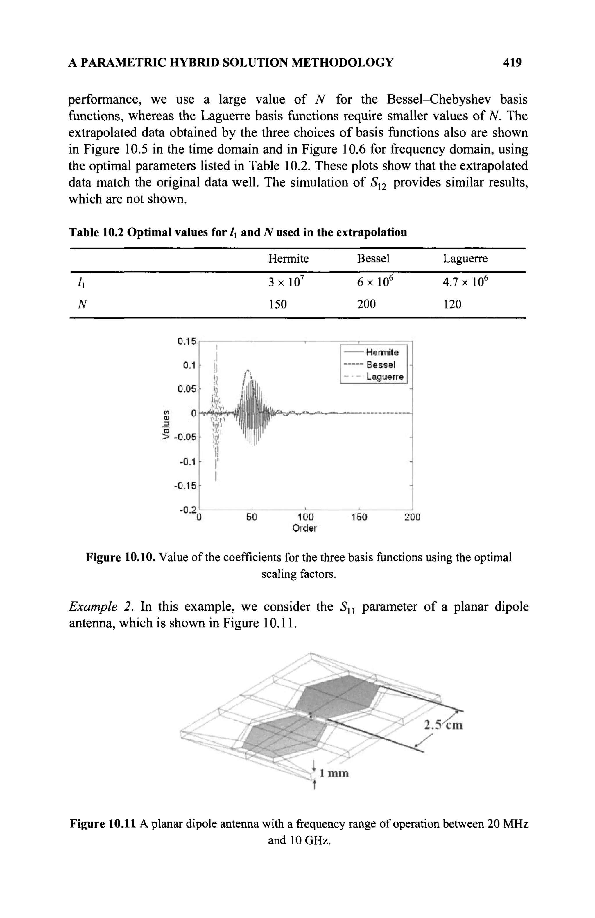
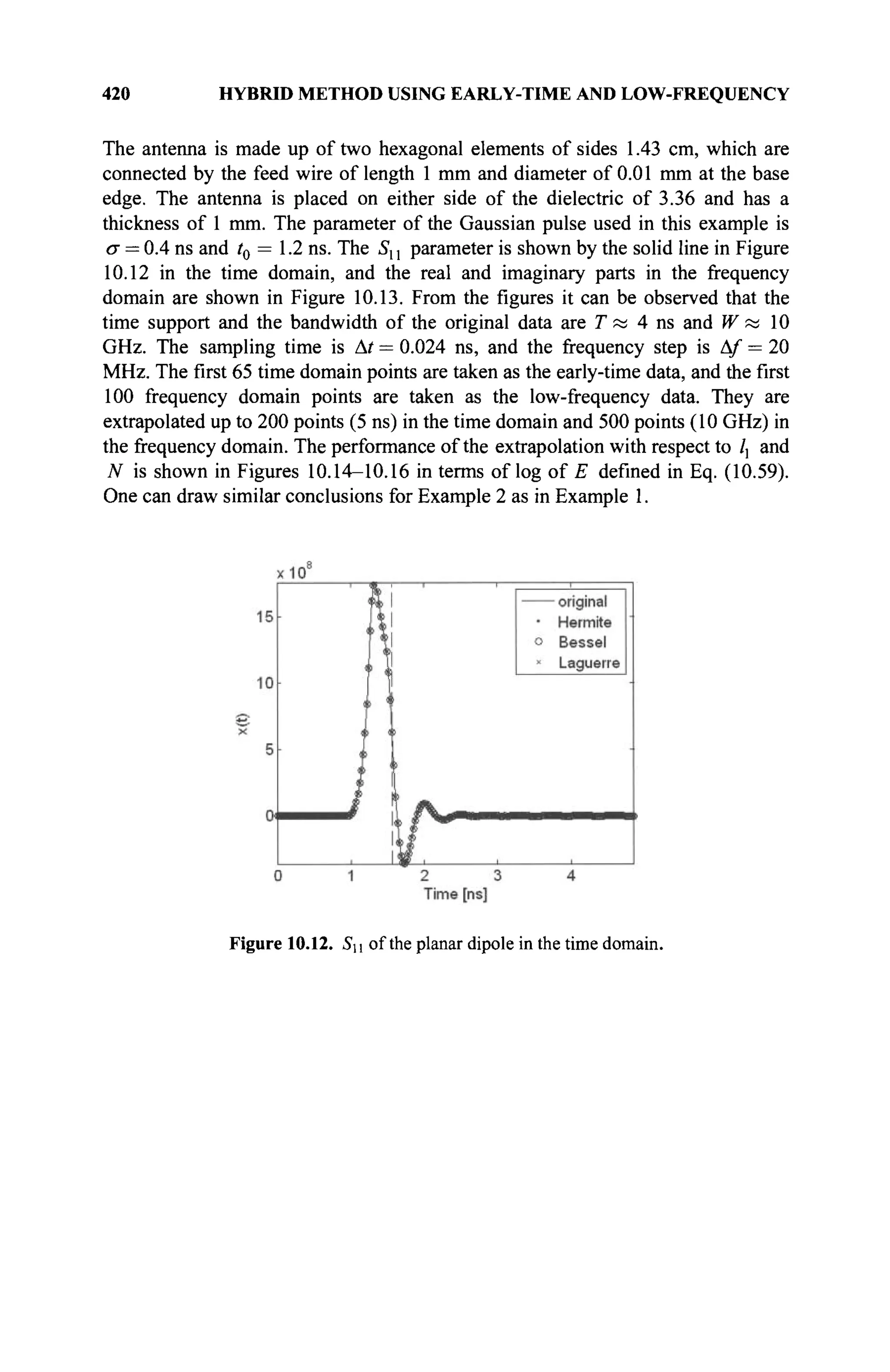
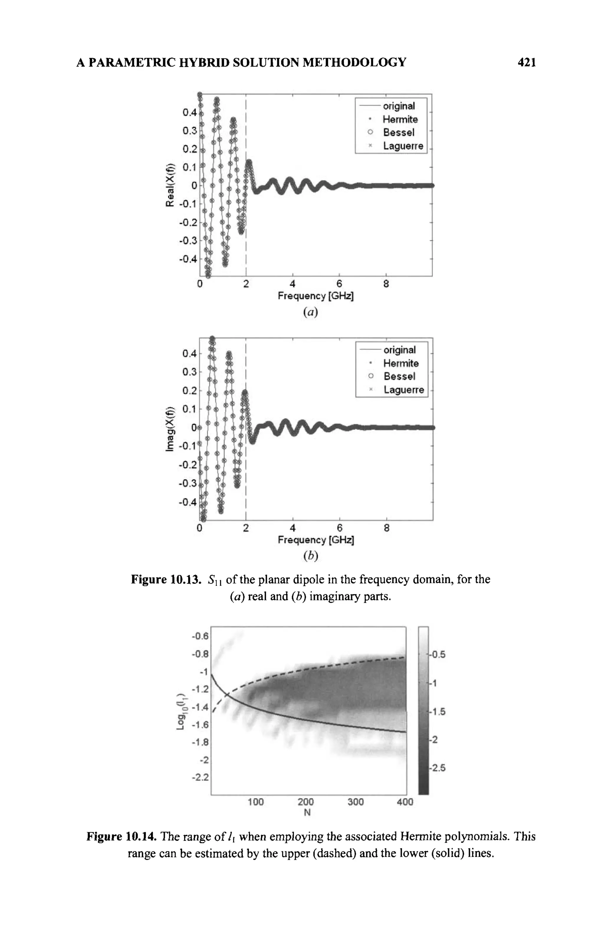
![422 HYBRID METHOD USING EARLY-TIME AND LOW-FREQUENCY
Figure 10.15. The range of l when employing the Bessel-Chebyshev functions. This range
can be estimated by the upper (dashed) and the lower (solid) lines.
Figure 10.16. The range oîlx when employing the associated Laguerre functions. This
range can be estimated by the upper (dashed) and the lower (solid) lines.
From this example, one can discuss the memory usage and the CPU time
gain that can be achieved by using the hybrid method across a purely time domain
or a frequency domain computational methodology. The dominant computational
load in the hybrid method is in the computation of the SVD of the matrix in Eq.
(10.6). It is a real matrix with dimension(Mj +2M2)xN. Because M,, M2, and
N are not large (usually around several hundreds), the CPU time for the
extrapolation is several seconds, which is negligible compared with the solution
time required for only the time domain or the frequency domain methods. For
MoM in the frequency domain, the number of unknowns, Un, is proportional to
the frequency of operation. The memory usage and the CPU time are proportional
to U2
n and U respectively. In this example, U„ =515 when generating the data
using the commercial EM software HOBBIES [1] upto 2 GHz, which is
considered to be the low-frequency data. The impedance matrix will occupy 4.2
Mb memory, and the problem will be finished in 3 seconds for one frequency. To
simulate the structure at the highest frequency (10 GHz), set Un = 2500, which
will occupy 100 Mb memory. The problem will execute for 60 seconds per](https://image.slidesharecdn.com/timeandfrequencydomainsolutionsofemproblemsusingintegralequationsandahybridmethodologyb-250205130750-568a5ba2/75/Time-and-Frequency-Domain-Solutions-of-EM-Problems-Using-Integral-Equations-and-a-Hybrid-Methodology-B-H-Jung-pdf-440-2048.jpg)
![A PARAMETRIC HYBRID SOLUTION METHODOLOGY 423
frequency, which is 20 times slower than analyzing the same problem at a low
frequency. If a large array of this antenna is simulated, the CPU time gain can be
up to 300 times. The memory usage gain is not obvious in the time domain
because a fine mesh is used at the highest frequency to obtain the early-time data.
However, this matrix can be saved to the hard disk, and the out-of-core solver can
be used [1]. In addition, the explicit MOT can be used to achieve the CPU time
gain because it does not require matrix inversion. The most important issue in time
domain is the instability in late time, and the hybrid method sometimes can
address this problem successfully. However, to obtain an accurate solution under
all circumstances, the MOD method is preferred over the MOT technique [25].
10.2.2 An Iterative Method to Find the Optimal Parameters
The objective of the hybrid method is to obtain the data for late-time and high-
frequency from the known early-time and low-frequency information. This
objective can be achieved as the data in early-time and low-frequency contain all
the necessary mutually complimentary information to characterize the system
electromagnetically, assuming a sufficient record length is available in both
domains. In that case, the error of the extrapolated data is computed only in early-
time and low-frequency, as the error of the extrapolation across the whole ranges
in both domains, and finds the minimum error to get the best performance. The
error is computed as follows. Take the Fourier transform of the data in the time
domain (both given and extrapolated) to obtain another set of data in the frequency
domain. Now compute the difference between the computed low-frequency data
from the time domain response and the given low-frequency data as follows:
Ef(li,N)-- ^[XexV'h'-T* Jwholespan Jjovvfrequency S i v e n
^ 'Ilow
frequency
2
(10.60)
where xex(t, Ιχ, Ν) is the given plus extrapolated data in the time domain and
^given(/) >s m e
giv e n
data in the frequency domain. Э is the Fourier transform
operator. This error is computed in terms of the S't norm from only the low-
frequency information. The error associated with the frequency domain data to
predict the early-time response is computed in a similar fashion. This is obtained
by extrapolating the frequency domain data and inverse Fourier transforming both
the given low-frequency and the extrapolated high-frequency information to the
time domain and computing the difference between this response and the given
early-time response. The error in the time domain is expressed as follows:
EtL->N)— M [ «(/''2'-^)wholespan Jearl time
x
given(0| early time (10.61)
where X^it, /]; N) is the extrapolated data in the frequency domain plus the
given low-frequency data, and xgven(t) is the given early-time data. Either Eqs.](https://image.slidesharecdn.com/timeandfrequencydomainsolutionsofemproblemsusingintegralequationsandahybridmethodologyb-250205130750-568a5ba2/75/Time-and-Frequency-Domain-Solutions-of-EM-Problems-Using-Integral-Equations-and-a-Hybrid-Methodology-B-H-Jung-pdf-441-2048.jpg)
![424 HYBRID METHOD USING EARLY-TIME AND LOW-FREQUENCY
(10.60) or (10.61) can be used to find the optimal value for /, and N when the
lowest error is achieved. This is accomplished by carrying out the computations
for all possible set is of parameters and then computing the following sum:
£'(/,, # ) = £}(/„ N) + E't{lu N) (10.62)
as the two errors in the time and frequency domains are complementary. It is
important to note, however, that the error given by Eq. (10.62) also can be
computed using either the S or the S^ norm. From a computational standpoint,
the matrix containing the unknown coefficients in Eq. (10.6) can be computed at
the highest value of N once, for every lx, to avoid repeated computations. Each
iteration will undertake only one matrix inversion. The whole search procedure
takes only a fraction of the time as compared with the solution of the original
electromagnetics problem caused by MoM or MOT/MOD, especially for
evaluating ultra-wide band responses of very complicated structures. Using Eq.
(10.62), one can estimate /] and N, which can yield values very close to the
optimal ones. Simulation results presented later in section 10.5 will validate the
concept of this method.
In summary, the optimal choice of the scaling parameter /, and N can
be obtained using the following recipe:
1. Determine the minimum degree Nmin as specified in Table 10.1.
There is no need to know the exact value of T and W of the data. A
range of the values of N from Nmin can be chosen for the
numerical search.
2. Use the error bound as given in Table 10.1 to determine the range of
/j in which the hybrid method will converge.
3. Search for the optimal values of /, and N by minimizing the error
in Eq. (10.62), by using the range of values of lx obtained at step 2
(and the range of N obtained in step 1).
Each of these three steps can be programmed easily and automatically, and the
computational cost is a minimum, as a small-dimensioned matrix equation of Eq.
(10.6) is solved. Here, the input required is the data specified in the early-time and
low-frequency, the sampling interval in time and frequency, AT and AF,
respectively, and the approximate time span T and the bandwidth W of the data.
Finally, these principles are illustrated using some numerical results.
Scattering from a dielectric hemisphere of 0.2 m diameter with er = 10 is
considered. The configuration of interest along with the discretization is shown in
Figure 10.17. The excitation arrives from the direction θ = 0, 0 = 0 (i.e., along
the negative z direction). The incident electric field is a Gaussian pulse, and it is
polarized along the x-axis. A frequency domain MoM EFIE formulation [1] is
used to compute the response in the low-frequency region. Also used is a MOT
time domain EFIE code [25] to obtain the early-time response. The time step used
in the MOT program is 266.7 ps. In this example, σ = 2 ns and t0 = 20 ns. E0 is](https://image.slidesharecdn.com/timeandfrequencydomainsolutionsofemproblemsusingintegralequationsandahybridmethodologyb-250205130750-568a5ba2/75/Time-and-Frequency-Domain-Solutions-of-EM-Problems-Using-Integral-Equations-and-a-Hybrid-Methodology-B-H-Jung-pdf-442-2048.jpg)
![A PARAMETRIC HYBRID SOLUTION METHODOLOGY 425
chosen to be 377 V/m. The time step ( At ) is dictated by the discretization used in
modeling of the geometry. The conjugate gradient method (CGM) has been used
to solve the matrix in Eq. (10.6) until the residue goes below ΙθΛ The
extrapolated time domain response is compared with the output of the time domain
response obtained from the MOT program [25], and the frequency domain
response is compared with that of the MoM code [1] and the discrete Fourier
transform of the time domain results. In all plots, the extrapolated signal refers to
the extrapolated response using all polynomial expansions, whereas the original
signal refers to the data obtained from the MOT or MoM codes. Also, the vertical
dotted lines in all figures indicate beyond which extrapolations have been
performed. The normalized error for the time and frequency domain data is
defined by Eq. (10.7).
Fig. 10.17 Discretization of a dielectric hemisphere.
Using the MOT algorithm, the time domain data for the electric and the
magnetic currents is obtained from t = 0 to / = 21.33 ns (80 data points). And the
frequency domain data is obtained from DC to / = 900.0 MHz (143 data points).
The results for only the electric current are plotted, as the result for the magnetic
current is similar. Assume that only the first 32 time-data points (up to t = 8.533
ns) and first 42 frequency-data points (up to / = 264.3 MHz) are available.
Solving the matrix equation, Eq. (10.6), using the available data, the time domain
response is extrapolated to 80 points (21.33 ns) and the frequency domain
response is extrapolated to 143 points (900.0 MHz).
Using the dimensionality theorem, choose N for this data set to be 42.
To examine how the error scales as a function of T
V
, change N from 5 to 200 with
an increment of 5. Hence, for a fixed scale factor, /,, simulations using 40
different values of N are carried out The values of the scale factor are set as
follows. The range of lx for the Laguerre and Bessel polynomials are varied from
1.5ΔΓχ10{0
·1_1>
~1.5АГх10!20хОЛ
"1}
.ТЬе range of /, for Hermite polynomials
are varied from 1.5ΔΓχ1001
~1.5Δ7:χ10{20χ01}
, as for the Hermite polynomials
it is larger than that of the other two polynomials. This implies that the scale factor
/, chosen at each step is incremented by the factor 10° '.](https://image.slidesharecdn.com/timeandfrequencydomainsolutionsofemproblemsusingintegralequationsandahybridmethodologyb-250205130750-568a5ba2/75/Time-and-Frequency-Domain-Solutions-of-EM-Problems-Using-Integral-Equations-and-a-Hybrid-Methodology-B-H-Jung-pdf-443-2048.jpg)
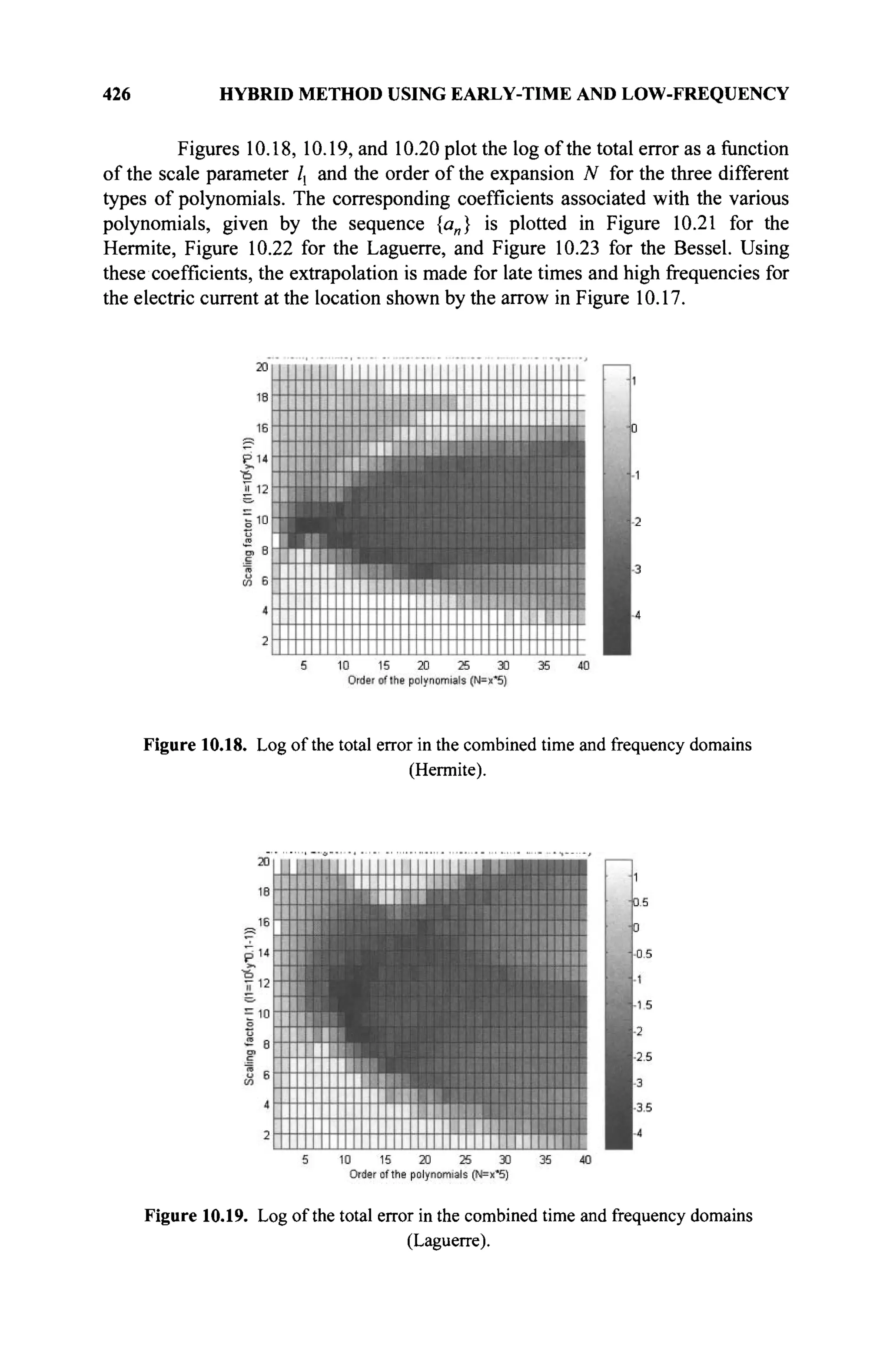
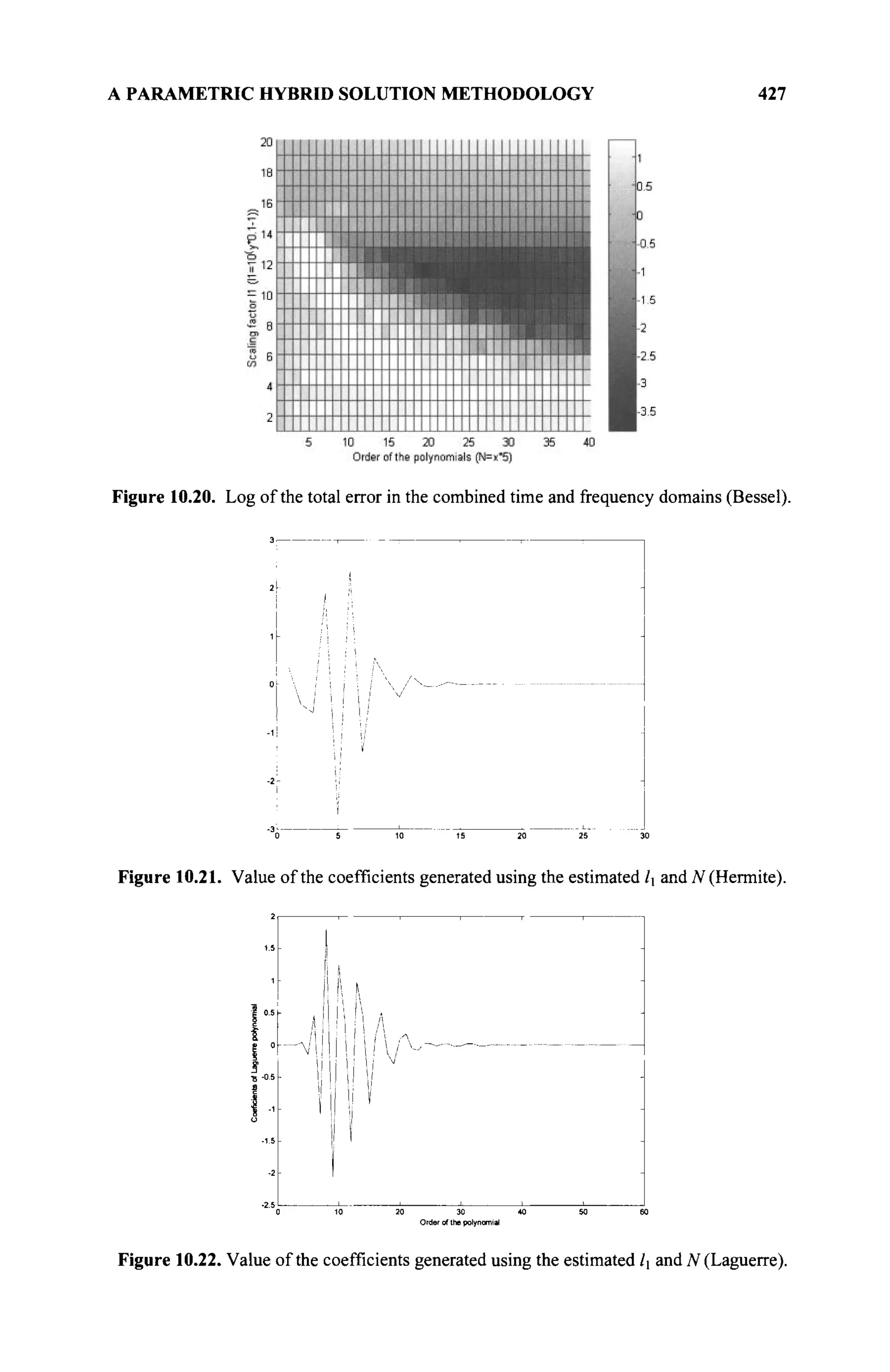
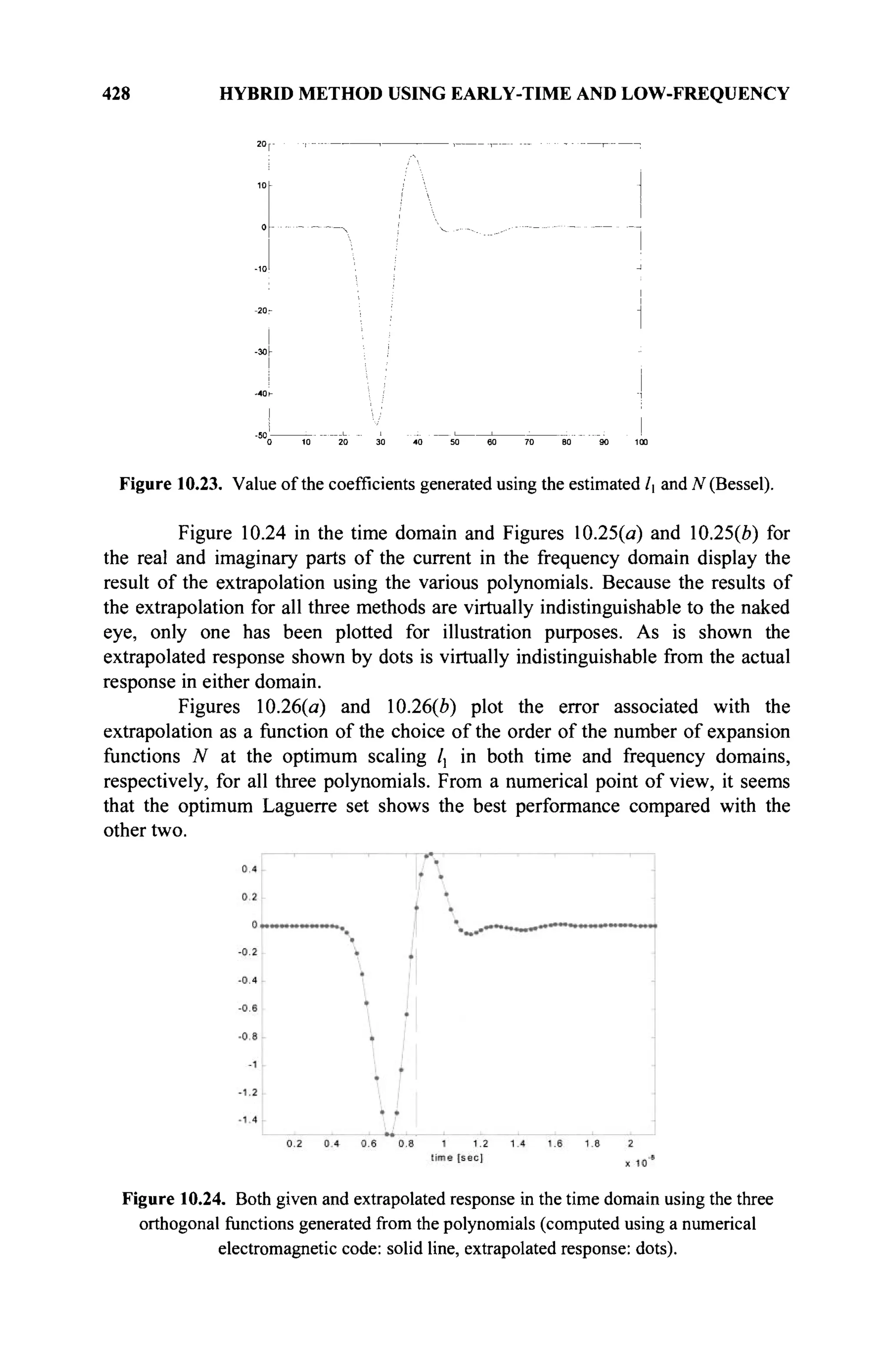
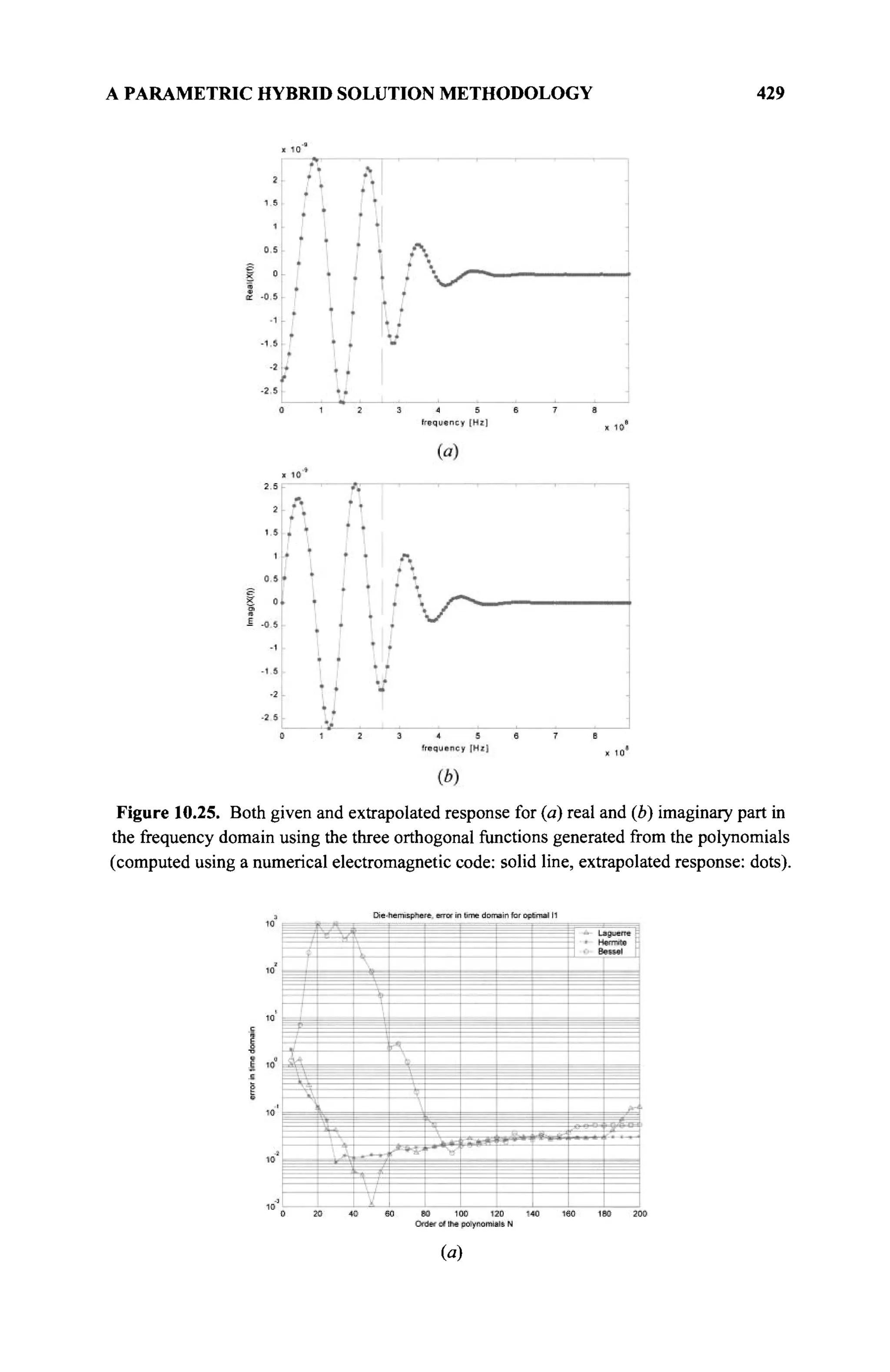
![430 HYBRID METHOD USING EARLY-TIME AND LOW-FREQUENCY
(*)
Figure 10.26. Error in the (a) time and (b) frequency domain plotted against the order of
the polynomial N for the optimum scale factor lx.
10.3 A NON-PARAMETRIC HYBRID METHODOLOGY
In this section, we look at nonparametric methods to carry out the simultaneous
extrapolation in the time and frequency domains using other mathematical
principles that need not be specified by certain parameters. For example, Adve and
Sarkar [4] developed an alternating projection method that enables a simultaneous
extrapolation of the early-time response in the time domain and the low-frequency
response in the frequency domain. The late-time domain solution may be
extrapolated further using the Matrix Pencil technique or the Hubert transform. In
the present section, it is observed that the alternating iterative method provided by
Adve and Sarkar is identical to the Neumann series solution of a second-kind
integral equation. Here it is demonstrated that this Neumann series solution is an
iterative error-reducing method.
It is anticipated that a more efficient iterative method is the conjugate
gradient method. For this procedure, it is shown that the governing operator is self-
adjoint and positive. The operator can be implemented by using the FFT and the
IFFT to improve the computational efficiency as will be illustrated.
The integral equations to be developed in this nonparametric solution
procedure are equivalent to the solution of a set of matrix equations. The
extrapolation then can be achieved by directly solving the matrix equation.
Although this matrix is ill-conditioned and rank deficient, good performance can
be achieved by using the SVD because of the special properties of the
extrapolation. Because small matrices are dealt with in this extrapolation
procedure, extraction of the early-time and low-frequency data by using the SVD
is also computationally efficient.
The problem formulation is provided in section 10.3.1, and then the
integral equation of the second kind is derived in section 10.3.2. The three direct
methods, Neumann iteration, conjugate gradient, and SVD are discussed
separately in sections 10.3.3-10.3.5. Finally, three more examples related to EM](https://image.slidesharecdn.com/timeandfrequencydomainsolutionsofemproblemsusingintegralequationsandahybridmethodologyb-250205130750-568a5ba2/75/Time-and-Frequency-Domain-Solutions-of-EM-Problems-Using-Integral-Equations-and-a-Hybrid-Methodology-B-H-Jung-pdf-448-2048.jpg)
![A NON-PARAMETRIC HYBRID METHODOLOGY 431
scattering are presented to validate the methods, and the performances of the three
methods are compared in section 10.3.6.
10.3.1 Formulation of the Problem
Assume that the Fourier transform of a causal function f(t), t G 5R+
, is given by
/(й>) = Э{/}(о))= Г +exp(-iû»/)/(0d/, ®eSR (ю.63)
The causal function f(t), is easily found from the inverse Fourier transform,
Д О = 9Г1
{/}(/) = - R e f T„+exp(ia*)/(û»)dû>, / € Ш +
(Ю.64)
where Re[·] denotes real part of. Furthermore, from Parseval's relation for causal
functions, the following is obtained:
Г m+ fit) g*(t)dt = -Re f , До) g » άω (10.65)
which will be used extensively in this section. The asterisk denotes the complex
conjugate. Now consider when f{a>) is known only in a bounded domain Ω, a
subdomain of 5ft+
. Denote the known functional values in Ω as /Ω{ύ)). This
results in,
ДЙ>) = /Д (Й»), о) еП (10.66)
Furthermore, assume that
Д 0 = /г(0, ' е Г (10.67)
where / r (t) is a known function in the bounded subdomain T of $R+
. Adve and
Sarkar [4] have developed an iterative scheme to determine /(/) for all t e 3î+
,
or f((o) for all <a € 9ft+
· To show that this iterative scheme is nothing but a
Neumann expansion of an integral equation of the second kind, the reconstruction
problem is formulated through an integral equation of the first kind as,
ft +exp(-ieot)f(t)dt = f Ω(ω), ω&Ω (10.68)
Because f(t) = fT(t) is known for t£T, Eq. (10.68) is rewritten as
fte Ш+Тexp(-iû*)/(0d/ = ΗΩ(ω), ω€Ω (10.69)](https://image.slidesharecdn.com/timeandfrequencydomainsolutionsofemproblemsusingintegralequationsandahybridmethodologyb-250205130750-568a5ba2/75/Time-and-Frequency-Domain-Solutions-of-EM-Problems-Using-Integral-Equations-and-a-Hybrid-Methodology-B-H-Jung-pdf-449-2048.jpg)
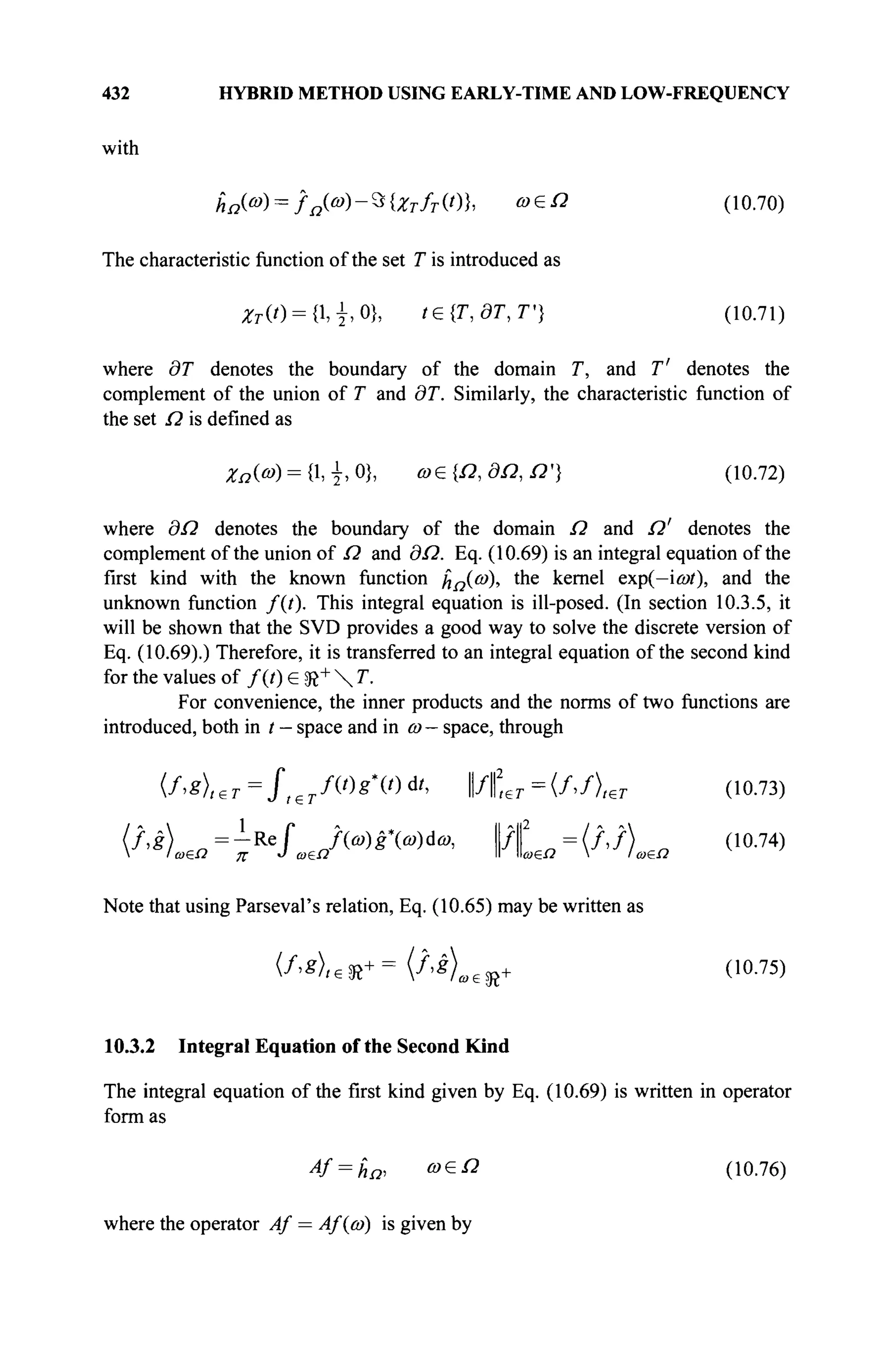
![A NON-PARAMETRIC HYBRID METHODOLOGY 433
4f = *{Q-zT)n (10.77)
The conversion of the first kind integral equation to that of the second kind is
similar to the conversion used by Van den Berg and Kleinman [26], Fokkema and
Van den Berg ([27], section 2.7) for convolution type operators, and Rhebergen et
al. [28]. First note that the operator Eq. (10.76) only holds for ω£Ω. Therefore
the equation is rewritten to one that holds for all ω G SR+
, viz.
4f = Zaha + 0--ZaW, « е Э ? +
(10.78)
Using Eq. (10.77), one can obtain
»{(Hfr)/} = ΖΩ&α + 0^ΖΩ)*{(^Ζτ)/}, о) G sft+ (10.79)
Because, this equation holds for all ω G sft+
, the inverse Fourier transformation is
taken on both sides to arrive at
(1-*г)/= Ъ-х
{Хпьп} + Ъ-х
{{-хп)Ъ{{-хт)Л}, /G5R+ (10.80)
By considering t G$t+
T only, this equation becomes an integral equation of
the second kind, and in operator notation, it is written as
f = g + Kf, t G SR+
V (10.81)
where
g = *~l
{Zaha) (10.82)
is the known function and
Κ/ = %-ι
{(1-χΩ)Ζ{(-χτ)/}} (10.83)
is the kernel operator.
10.3.3 The Neumann Expansion
First, observe that the integral equation of the second kind, Eq. (10.71), and can be
solved iteratively using the Neumann iterative solution as
/ o = 0 , f„=g + Kf„-i, 1
1 = 1,2,- (10.84)
At the «th step, the residual error is defined as](https://image.slidesharecdn.com/timeandfrequencydomainsolutionsofemproblemsusingintegralequationsandahybridmethodologyb-250205130750-568a5ba2/75/Time-and-Frequency-Domain-Solutions-of-EM-Problems-Using-Integral-Equations-and-a-Hybrid-Methodology-B-H-Jung-pdf-451-2048.jpg)
![A NON-PARAMETRIC HYBRID METHODOLOGY 435
inverse Fourier transforms. The Fourier transform is performed on the late-time
data /„, and add the high-frequency component of the transform with the known
low-frequency component. The scheme can be modified to compute updates for
/„ , t € SR+, by observing that hn=fü-F {χτ/τ } and
ίη={^Χτ)ί«+Χτίτ, 'esR+ (10.92)
This scheme is presented in Table 10.4. Obviously, this latter scheme is identical
to the one described in Ref. [2].
Table 10.3 Neumann iterative scheme for fn, t G $l+
T
t -domain ω -domain
/и-1
I
x ( l - ^ r )
fn
* ( l - * o )
I
+Zn>b
Table 10.4 Iterative scheme for fn,t£ 5J+
t -domain ω -domain
fn-
I
* ( ! - ; & ■ )
I
+XTJT
fn
x ( l - 2 n )
I
+Xnki
It is also observed that the Neumann iterative solution can be written as
f=EK
"s
л=0
(10.93)
which is a representation in the Kjylov subspace spanned by
{K"g, n = 0, 1, 2, ...}. If the error reduction of the Neumann iteration is very
slow, then it can be speeded up by using more advanced Krylov-subspace methods](https://image.slidesharecdn.com/timeandfrequencydomainsolutionsofemproblemsusingintegralequationsandahybridmethodologyb-250205130750-568a5ba2/75/Time-and-Frequency-Domain-Solutions-of-EM-Problems-Using-Integral-Equations-and-a-Hybrid-Methodology-B-H-Jung-pdf-453-2048.jpg)
![436 HYBRID METHOD USING EARLY-TIME AND LOW-FREQUENCY
(e.g., over-relaxation and successive over-relaxation methods [29]). Experience
has taught that a conjugate gradient method can be used advantageously.
10.3.4 The Conjugate Gradient Method
Before the conjugate gradient (CG) method is discussed, the integral equation of
Eq. (10.81) can be rewritten as
Lf = g, t£ft+
T (10.94)
with L = I — K , where / is the identity operator. Now, observe
Lf = ^{Zn%{V-Zr)f}} (10.95)
This operator is equivalent to
Lf = J,^C(t-t')f(t')dt' (10.96)
where
C(t)--
0, t<0
(10.97)
For the CG method to be discussed, the adjoint operator LH
of L is defined
through
Using Eq. (10.95) in Eq. (10.98) and the Parseval's relation results in
= <3 Ю-Ζτ )/}, Zn 3 W-Ζτ )g})w e JJ+
= (V-ZT)A 3 _ 1
{Zo Щ1-Хт)8)}) ю +
= (f>L
g)l€%+T (10.99)
which shows that L is self-adjoint (L = L). Subsequently, it will be proven that
the operator L is positive by showing that the inner product](https://image.slidesharecdn.com/timeandfrequencydomainsolutionsofemproblemsusingintegralequationsandahybridmethodologyb-250205130750-568a5ba2/75/Time-and-Frequency-Domain-Solutions-of-EM-Problems-Using-Integral-Equations-and-a-Hybrid-Methodology-B-H-Jung-pdf-454-2048.jpg)
![A NON-PARAMETRIC HYBRID METHODOLOGY 437
= {Zn 9f{(l-^)/}, *{(^Ζτ)/})α€χ+
= Ρ{(1-Ζτ)/}ω£Ω>0 (10.100)
for / ^ 0 everywhere in sft"t
"J'. Convergence of the conjugate gradient method
(CG) for positive operators has been established in Ref. [30]. The conjugate
gradient iterative scheme to solve Eq. (10.94) is given subsequently. It minimizes
the inner product ( / — /„, L(f — /„ )) «л+ г · The initial estimate is started with
/ 0 = 0 , r0=h = F-l
{Xnfn}
1 Ы , е й + г =
I N L s R + r (10.101)
Next the scheme chooses
H - ' o
II Il2
/ < v
i > L v
i > , f
/ i = / o + « i v
i
η rrro-α,Ζ,ν, (10.102)
and computes successively for n = 2, 3, ..
1,едг+Г/1Г«-2|1геЭг+Г
r
n-1,p so+Г /lk-2 ,p «>+T)v
«-i
«и - lk-iII,e sß+r/(v
»'i v
»),e sß+r
»·Λ =';,-ι-α^νΙ Ι (10.103)
in which
I*Vn=S*~l
{Za%{Q-zM} (10-104)
In this CG scheme, the operator Lvn only consists of the forward and inverse
Fourier transforms of causal functions, defined in Eqs. (10.63)—(10.64). In
computer simulations, the FFT and IFFT [31] can be used to implement the
Fourier transform. Because it is not possible to deal with FFT or IFFT of the data
/ which has infinite length, it is assumed that / has a finite support Wt. For
t > Wt, it is assumed that f(t) « 0. It is reasonable to assume that this is true for](https://image.slidesharecdn.com/timeandfrequencydomainsolutionsofemproblemsusingintegralequationsandahybridmethodologyb-250205130750-568a5ba2/75/Time-and-Frequency-Domain-Solutions-of-EM-Problems-Using-Integral-Equations-and-a-Hybrid-Methodology-B-H-Jung-pdf-455-2048.jpg)
![438 HYBRID METHOD USING EARLY-TIME AND LOW-FREQUENCY
most EM analysis [13]. Similarly, it also is assumed that/has finite bandwidth so
that Wf (f(a>) « 0 for ω < Wf ). The latter is always true, as the structures are
discretized spatially based on the highest frequency of interest.
10.3.5 Equivalent Matrix Formulations and Solution Using the SVD
It is assumed that discrete samples of the data are available. Apply the discrete
Fourier transform (DFT) to the sampled data. The sampling time At is assumed to
be sufficiently small. Suppose the sampled data sequence of / in the time domain
is x, with the length Mt, and the sequence in the frequency domain is X, with
the length Mf. The early-time data x, is obtained up to Mx data points. The next
step is to extrapolate the late-time data x2 with the length of Mt — Mx. Similarly,
extrapolate the high-frequency data X2 (with the length M{ — M, ) using the low-
frequency data X] (with the length Μγ ). Ref. [4] discussed how to choose M,
and M2 to obtain good performance. Experience shows that a high quality of
extrapolation usually can be obtained if we choose the early-time to contain
response later in time than the peak in the excitation, and the low-frequency data
should be larger in size containing at least the first resonant frequency of the
structure. However this restriction is flexible because we can reduce M, by
increasing M2 ■ We now define the data sequences as
* = {/(0), /(Δ/), - , / P r 1)Δ0, f{MxM), - , f((M, - 1)Δ0}Γ
X = {/(0), / ( A/),. · -, Л(М2 -1)ДО, f(M2Af),-,f((Mf-)Af)}T
(10.105)
where Af is the sampling interval in the frequency domain, and the superscript
T denotes the transpose of a vector or matrix. Performing the DFT to a vector x is
equivalent to multiplication of x with the DFT matrix KDFT. The vectors X and
x are related by
X = KDFTx (10.106)
where the DFT matrix KDFT can be defined and partitioned as
1 1 ·■· 1
-J2n,
M-fM2- -βπΙ
Μχ/Μ2- ... ~ί'1πί
Μ,-ίΜ2-
-;'2π/Μι_ι/Μ2 -j2ntMxfMl ^ -Jlnt
M,-fM2
-Jl"tM~fMf~ -J^'M^fUf-X ~J2
'ri
Ml-fMf-l
К DFT](https://image.slidesharecdn.com/timeandfrequencydomainsolutionsofemproblemsusingintegralequationsandahybridmethodologyb-250205130750-568a5ba2/75/Time-and-Frequency-Domain-Solutions-of-EM-Problems-Using-Integral-Equations-and-a-Hybrid-Methodology-B-H-Jung-pdf-456-2048.jpg)
![440 HYBRID METHOD USING EARLY-TIME AND LOW-FREQUENCY
conjugate gradient method thus is established. Furthermore, by looking at any
element of the matrix DA, which is given by
it is clear that it is only dependent on (m — n). Hence, DA is a Toeplitz matrix.
Therefore, the CGM-FFT method can be implemented to reduce the computational
load. The recipe is similar to that outlined in section 10.3.4, and the result should
be exactly the same. Instead of solving Eq. (10.111), in this section, the feasibility
of solving Eq. (10.109) is discussed directly.
Matrix A contains integer powers of the phasor β~^2πΑιί
^. It is an ill-
conditioned matrix. Furthermore, M2 necessarily is not equal to (M, — M{), so
that A may be rank-deficient. SVD is a stable method for solving ill-conditioned
matrix equations in a least-square sense [32]. Among the solutions of Eq. (10.109),
SVD will provide the solution of x2
w
i m a s
small a norm as possible. This
property is important for the extrapolation. The feasibility of the extrapolation is
based on the assumption that the low-frequency data consists of the late-time
information and vice versa. Using SVD, the norm or the energy of x2 will be
minimized under the condition of Eq. (10.109). Eq. (10.109) guarantees that x2
contains the information of the low-frequency data, and SVD makes sure that x2
does not contain any information about the high-frequency (SVD minimizes the
energy of x2 )· Hence, the solution of Eq. (10.109) by SVD should be what we
want in an extrapolation. Simulation results in section 10.3.6 will validate this
explanation.
Another advantage of using SVD is that we can decide when we have
sufficient data by analyzing the distribution of the singular values. If the smallest
singular value is not of the same order in magnitude as the noise in the data then
there is not enough data to carry out the extrapolation. More data must be
generated either in the time domain or in the frequency domain, which means
either M, or M2 need to be increased.
Although the computational load of a SVD is of the order of 0{mn2
) for
an /и x« matrix, it will not be much for the extrapolation problem; M2 and
M, - Mx is of the order of 102
. The CPU times used for SVD and the CG method
are similar. If the data ( Xj and X] ) that is obtained from an EM computation are
not accurate (e.g., there are some perturbations in X! ), then stable solutions still
can be obtained if some threshold is set for the singular values of A. To avoid
computational errors, Eq. (10.109) is separated into real and imaginary parts, and
one solves the following real matrix equation:
Re (A)
Im(A)
Re(X1 -Bx1 )
I m ^ - B x , )
(10.113)](https://image.slidesharecdn.com/timeandfrequencydomainsolutionsofemproblemsusingintegralequationsandahybridmethodologyb-250205130750-568a5ba2/75/Time-and-Frequency-Domain-Solutions-of-EM-Problems-Using-Integral-Equations-and-a-Hybrid-Methodology-B-H-Jung-pdf-458-2048.jpg)
![A NON-PARAMETRIC HYBRID METHODOLOGY 441
10.3.6 Numerical Implementation and Results
In this section, three representative scattering structures are considered to validate
the formulations. They are a sphere, an electrically large cube, and a dipole
mounted on the top of a car. The goal is to extrapolate the induced surface current
or the scattered field by the structure using early-time and low-frequency data and
compare it with the results obtained using a MoM [1] solution in the frequency
domain and DFT of the MOT solution in the time domain. The extrapolated time-
domain response is compared with the results obtained using the MOT [7] and
inverse discrete Fourier transform (IDFT) of the complete frequency-domain data.
Note that when MOT is used to calculate the early-time data, the mesh size of the
structure should be determined at the highest frequency considered in the analysis.
The highest frequency is determined by the spatial discretization of the structure
and vice versa. In all the figures showing the current or the field data, the vertical
line represents the partition to the left of which is the data given and to the right is
the extrapolated data.
A Gaussian pulse is used as the incident plane wave in the time domain.
It has the following form:
1 -M*
s(t) = -^=U0e^"> (10.114)
where σ is proportional to the width of the pulse. The time t0 is the delay to make
s(t) к 0 for t < 0. U0 is a scalar amplitude. In frequency domain, the pulse has a
spectrum
s(/) = t V [ 4
+JWO (10.115)
Note that S(f) is approximately band limited to 1/σ.
To evaluate the performance of the extrapolation, we use the following
normalized mean square error (MSE):
MSE = ^ ~ * 2
^ 2
(10.116)
Ык
where || · || is the S^ norm of a vector. For the Neumann iteration, up to n = 1000
steps was used in Eq. (10.84). For the CG method, the iteration is repeated until
the normalized error
ErJls-γΊί (ШЛИ,
hi](https://image.slidesharecdn.com/timeandfrequencydomainsolutionsofemproblemsusingintegralequationsandahybridmethodologyb-250205130750-568a5ba2/75/Time-and-Frequency-Domain-Solutions-of-EM-Problems-Using-Integral-Equations-and-a-Hybrid-Methodology-B-H-Jung-pdf-459-2048.jpg)
![442 HYBRID METHOD USING EARLY-TIME AND LOW-FREQUENCY
becomes less than 10 .
Example 3. A conducting sphere: In this example, a conducting sphere with
diameter 0.2 m is positioned at the origin as shown in Figure 10.27. An excitation
plane wave is incident along the -x direction and is polarized along the y direction.
The parameter of the incident Gaussian pulse used in this example is σ — 1.7 ns
and t0 =3.4 ns. Observe that the induced current in the middle of the shaded plate
is considered to be the data of interest. The current is shown in Figure 10.28 in the
time domain and in Figure 10.29 for the frequency domain. The sampling time At
= 0.0293 lm (1 lm = 3.33 ns), and the frequency step Af = 20 MHz. The first 35
time domain points are taken (up to 0.996 lm) as the early-time data and the first
35 frequency domain points (up to 0.68 GHz) as the low-frequency data, and we
extrapolate them up to 128 points (3.72 lm) in the time domain and 128 points
(2.54 GHz) in the frequency domain. It takes 163 iterations for the CG method to
converge. Figure 10.28 also illustrates that the extrapolated data agrees well with
the original data for all the three methods. The SVD has the minimum MSE and
the performance of the Neumann iteration is the worst. The MSEs for the three
methods are shown in the legend. The performance by SVD (MSE is of the order
of 10~ ) is similar to the extrapolation by the orthonormal functions with the
optimal scaling factor and optimal number of basis functions [15-17]. The
extrapolated data also can be obtained from the FFT of the total data in the time
domain.
Example 4. An electrically large cube: In this example, a 1 m x 1 m x 1 m
conducting cube is positioned at the origin as shown in Figure 10.30. The incident
plane wave is arriving along -x direction and is polarized along the y direction.
The parameter of the incident Gaussian pulse used in this example is σ = 0.1335
ns and t0 = 1.068 ns. Its bandwidth is approximately 1/σ= 7.5 GHz. The
wavelength λ in air at 7.5 GHz is 0.04 m. Hence, the cube is approximately 25Д
long at the highest frequency. Consider the reflected field along +x direction as the
original data. The scattered field (the dominant polarization is in the z direction) is
shown in Figure 10.31 in the time domain and in Figure 10.32 for the frequency
domain. The sampling time At = 0.0073 lm (1 lm = 3.33 ns), and the frequency
step Af = 20 MHz. Because the structure is large compared with the wavelength,
most of the energy exciting the cube is reflected back from the front plate. The
effect is equivalent to taking a time derivative, which dominates the early-time
response. However, the resonance effect from the late time data can be observed
way out along the time axis. A change from positive to negative "DC" field occurs
around 4.43 ns. The delay between this change and t0 is the round trip time for the
surface current from the center to the edge of the front plate (1 m). This is the
signature of a conducting plate. A small late pulse appears at 7.76 ns, the delay of
which from t0 is 6.69 ns. During this delay, the wave travels 2 m, which is the
round trip time taken to travel from the front to the rear plate. This is the signature
of the cube. In the frequency domain, the higher order resonances are small ripples
in Figure 10.32. The first 40 time domain samples (up to 0.293 lm) are taken as the](https://image.slidesharecdn.com/timeandfrequencydomainsolutionsofemproblemsusingintegralequationsandahybridmethodologyb-250205130750-568a5ba2/75/Time-and-Frequency-Domain-Solutions-of-EM-Problems-Using-Integral-Equations-and-a-Hybrid-Methodology-B-H-Jung-pdf-460-2048.jpg)
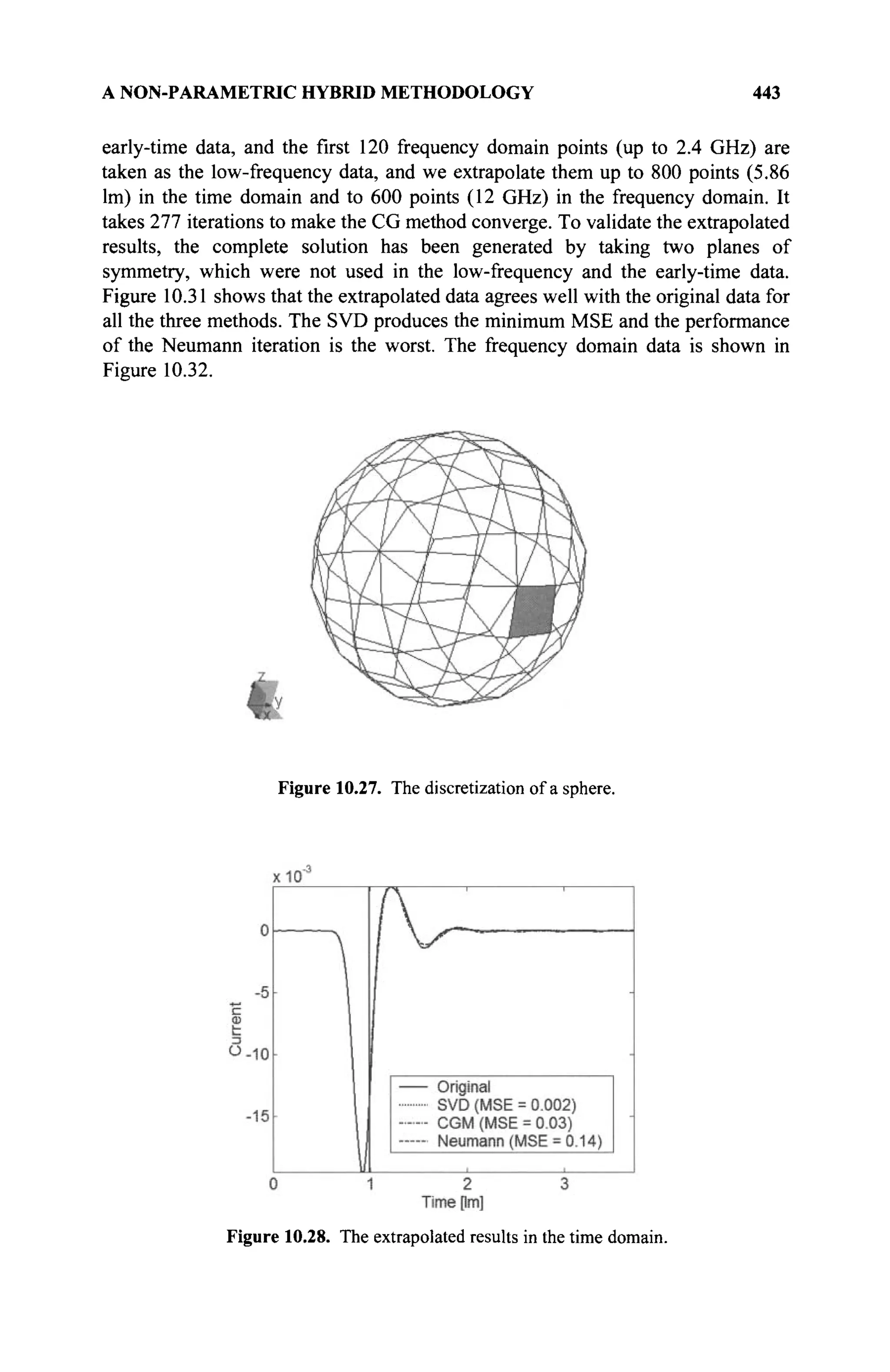
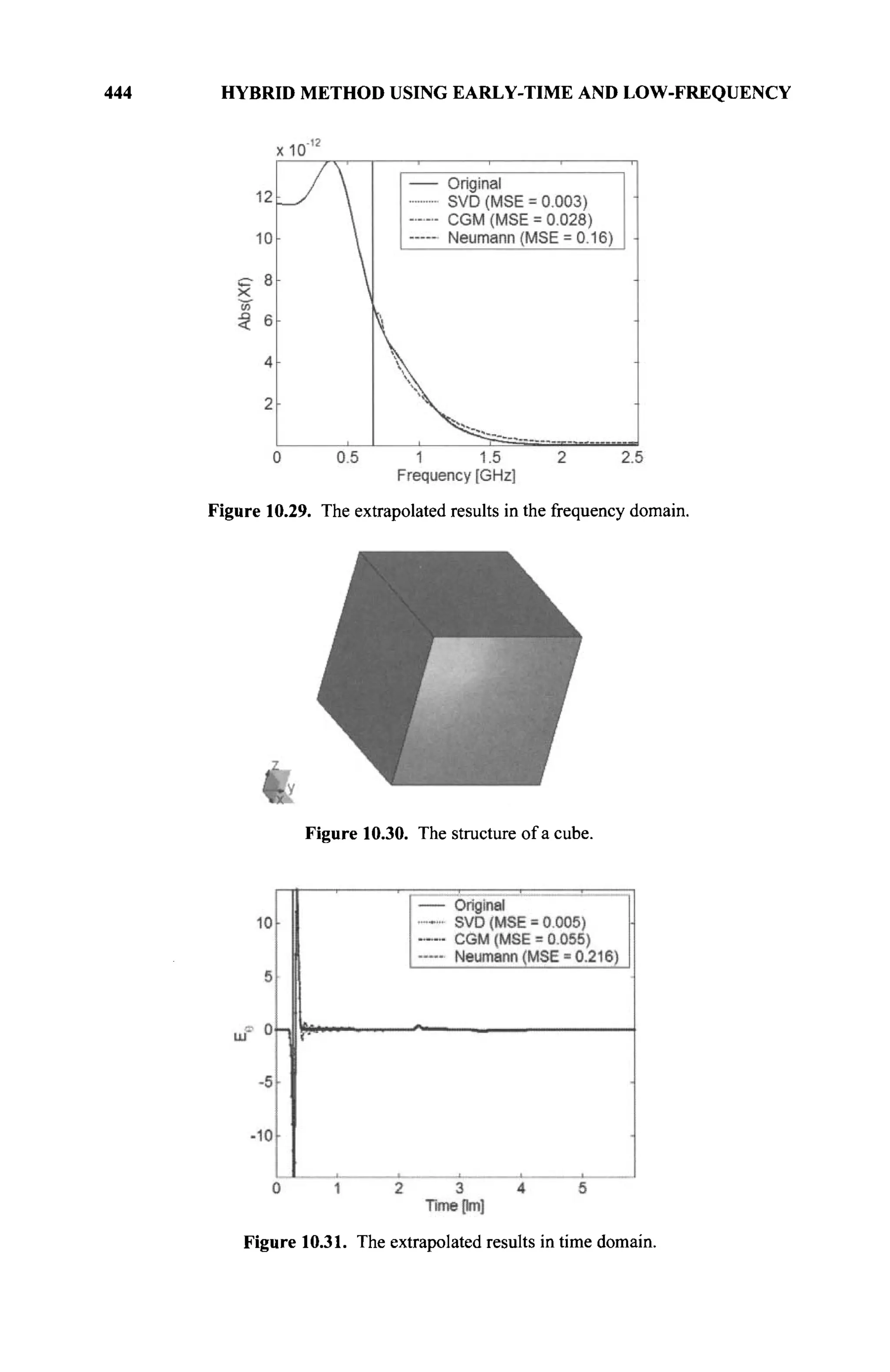
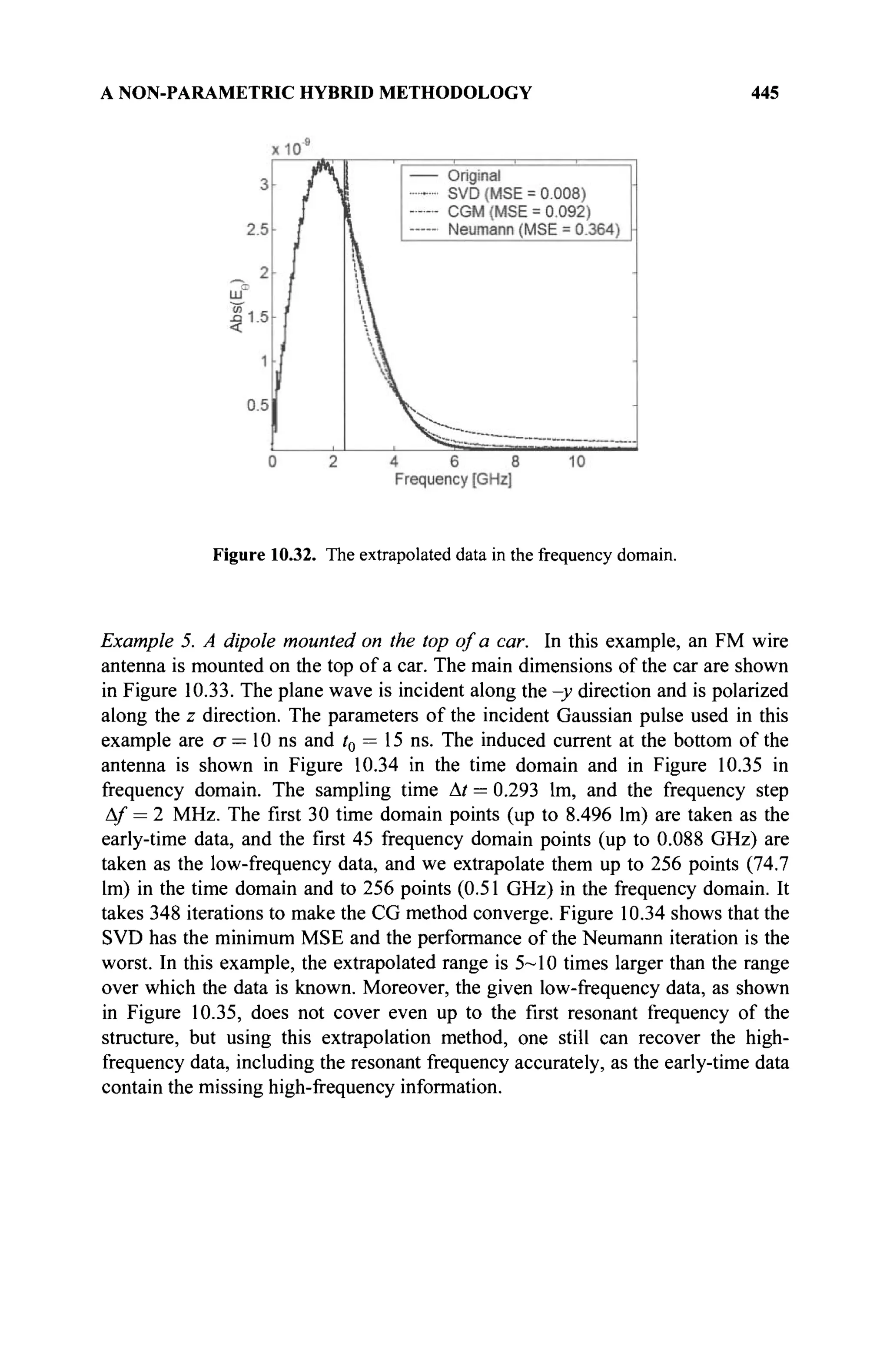
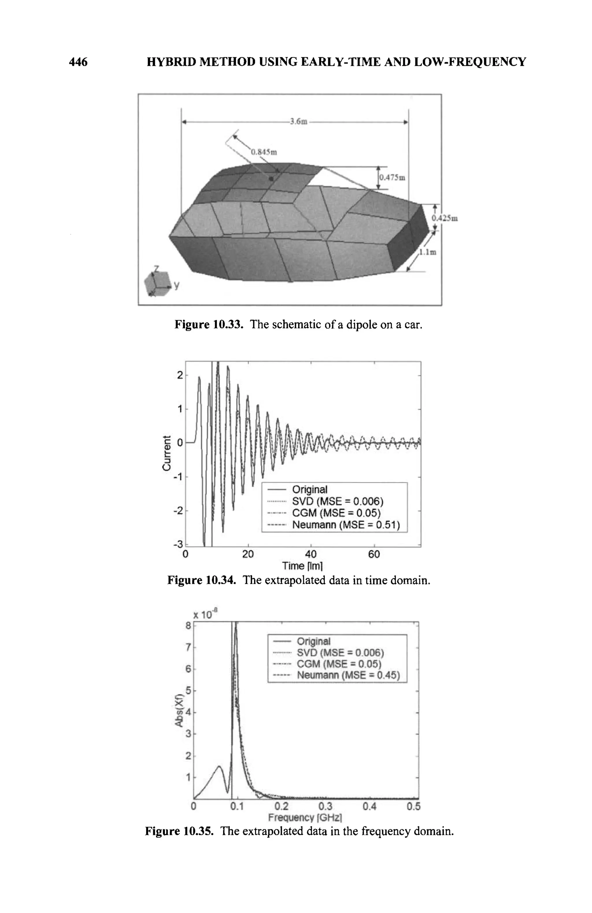
![448 HYBRID METHOD USING EARLY-TIME AND LOW-FREQUENCY
cannot be solved exclusively in either the time or in the frequency domain, even
when using a supercomputer.
REFERENCES
[I] Y. Zhang and T. K. Sarkar, Parallel Solution of Integral Equation-Based EM
Problems in the Frequency Domain, John Wiley and Sons, New York, 2009.
[2] R. S. Adve, T. K. Sarkar, S. M. Rao, E. K. Miller, and D. Pflug, "Application of the
Cauchy method for extrapolating/interpolating narrowband system responses,"
IEEE Trans, on Microwave Theory Tech. Vol. 45, pp. 837-845, 1997.
[3] E. K. Miller and T. K. Sarkar, "an introduction to the use of model-based parameter
estimation in electromagnetics," in W. R. Stone (ed.) Review of Radio Science
1996-1999, Oxford University Press, N.Y., pp. 139-174. 1999.
[4] R. S. Adve and T. K. Sarkar, "Simultaneous time and frequency domain
extrapolation," IEEE Trans, on Antennas Prop., Vol. 46, pp. 484-493, 1998.
[5] S. Narayana, S. M. Rao, R. S. Adve, T. K. Sarkar, V. Vannicola, M. Wicks, and S.
Scott, "Interpolation/Extrapolation of frequency responses using the Hubert
transform," IEEE Trans, on Microwave Theory Tech., Vol. 44, pp. 1621-1627,
1996.
[6] S. Narayana, T. K. Sarkar and R. S. Adve, "A comparison of two techniques for the
interpolation/extrapolation of frequency domain responses," Digit. Signal Procès.,
Vol. 6, pp. 51-67, 1996.
[7] T. K. Sarkar, W. Lee, and S. M. Rao, "Analysis of transient scattering from
composite arbitrarily shaped complex structures," IEEE Trans, on Antennas and
Prop., Vol. 48, pp. 1625-1634, 2000.
[8] S. M. Rao and T. K. Sarkar, "Implicit solution of time domain integral equations for
arbitrarily shaped dielectric bodies," Microwave Opt. Techno. Let., Vol. 21, pp.
201-205, 1999.
[9] R. S. Adve, T. K. Sarkar, O. M. Pereira-Filho, and S. M. Rao, "Extrapolation of
time domain responses from three dimensional conducting objects utilizing the
matrix pencil technique," IEEE Trans, on Antennas Prop., Vol. 45, pp. 147-156,
1997.
[10] T. K. Sarkar and O. M. Pereira-Filho, "Using the matrix pencil method to estimate
the parameters of a sum of complex exponentials," IEEE Trans, on Antennas Prop.,
Vol. 37, pp. 48-55, 1995.
[II] M. M. Rao, T. K. Sarkar, T. Anjali, and R. S. Adve, "Simultaneous extrapolation in
time and frequency domains using Hermite expansions," IEEE Trans, on Antennas
Prop., Vol. 47, pp. 1108-1115, 1999.
[12] M. M. Rao, T. K. Sarkar, R. S. Adve, T. Anjali, and J. F. Callejon, "Extrapolation
of Electromagnetic responses from conducting objects in time and frequency
domains," IEEE Trans, on Microwave Theory Tech., Vol. 47, pp. 1964-1974, 1999.
[13] T. K. Sarkar, J. Koh, W. Lee, and M. Salazar-Palma, "Analysis of electromagnetic
systems irradiated by ultra-short ultra-wideband pulse," Meas. Sei. & Tech., Vol.
12, pp. 1757-1768,2001.
[14] T. K. Sarkar and J. Koh, "Generation of a wide-band electromagnetic response
through a Laguerre expansion using early-time and low-frequency data," IEEE
Trans. Microwave Theory Tech., Vol. 50, pp. 1408-1416, 2002.
[15] M. Yuan, A. De, T. К. Sarkar, J. Koh, and В. Н. Jung, "Conditions for generation
of stable and accurate hybrid TD-FD MoM solutions," IEEE Trans. Microwave
Theory Tech., Vol. 54, pp. 2552-2563, 2006.](https://image.slidesharecdn.com/timeandfrequencydomainsolutionsofemproblemsusingintegralequationsandahybridmethodologyb-250205130750-568a5ba2/75/Time-and-Frequency-Domain-Solutions-of-EM-Problems-Using-Integral-Equations-and-a-Hybrid-Methodology-B-H-Jung-pdf-466-2048.jpg)
![REFERENCES 449
[16] M. Yuan, J. Koh, T. K. Sarkar, W. Lee, and M. Salazar-Palma, "A comparison of
performance of three orthogonal polynomials in extraction of wide-band response
using early time and low frequency data," IEEE Trans. Antennas and Prop., Vol.
53, pp. 785-792, 2005.
[17] M. Yuan, T. K. Sarkar, B. H. Jung, Z. Ji, and M. Salazar-Palma, "Use of discrete
Laguerre sequences to extrapolate wide-band response from early time and low
frequency data," IEEE Trans, on Microwave Theory Tech., Vol. 52, pp. 1740-1750,
2004.
[18] M. Yuan, P. M. van den Berg, and T. K. Sarkar, "Direct extrapolation of a causal
signal using low-frequency and early-time data," IEEE Trans, on Antennas Prop.,
Vol. 53, pp. 2290-2298, 2005.
[19] G. H. Golub and С F. Van Loan, Matrix Computations, Johns Hopkins University
Press, Baltimore, M.D., 1991.
[20] D. Slepian, "Prolate spheroidal wave functions, Fourier analysis, and uncertainty-V:
The discrete case," Bell Sys. Tech. J., Vol. 57, pp. 1371-1430, 1978.
[21] D. Slepian, "On bandwidth," Proc. IEEE, Vol. 64, pp. 292-300, 1976.
[22] M. A. Masnadi-Shirazi and N. Ahmed, "Optimum Laguerre networks for a class of
discrete-time systems," IEEE Trans. Signal Processing, Vol. 39, pp. 2104-2108,
1991
[23] A. D. Poularikas, The Transforms and Applications Handbook, IEEE Press,
Washing, D.C., 1996.
[24] B. H. Jung and T. K. Sarkar, "Transient scattering from three-dimensional
conducting bodies by using magnetic field integral equation," J. Electromagn.
Waves Appi, Vol. 16, pp. 111-128,2002.
[25] B. H. Jung, Y. S. Chung, and T. K. Sarkar, "Time-domain EFIE, MFIE, and CFIE
formulations using Laguerre Polynomials as temporal basis functions for the
analysis of transient scattering from arbitrarily shaped conducting structures,"
Progress in Electromagnetics Research, Vol. 39, pp. 1-45, 2003.
[26] P. M. van den Berg and R. E. Kleinman, "The Conjugate gradient spectral iterative
technique for planar structures," IEEE Trans. Antennas and Prop., Vol. 36, pp.
1418-1423,1988.
[27] J. T. Fokkema and P. M van den Berg, Seismic Applications of Acoustic
Reciprocity, Elsevier, Amsterdam, The Netherland, 1973.
[28] J. B. Rhebergen, P. M. van den Berg and T. M. Habashy, "Iterative reconstruction
of images from incomplete spectral data," Inverse Probl, Vol. 13, pp. 829-842,
1997.
[29] R. E. Kleinman and P. M. van den Berg, "Iterative methods for solving integral
equations," Radio Sei, Vol. 26, pp. 175-181, 1991.
[30] T. K. Sarkar (ed.), Application of Conjugate Gradient Method to Electromagnetics
and Signal Analysis, Elsevier, New York, 1991, pp. 67-102.
[31] E. O. Brigham, The Fast Fourier Transform, Prentice-Hall, Englewood Cliffs N.J.,
1974.
[32] L. N. Trefethen and D. Bau III, Numerical Linear Algebra, SIAM, Philadelphia,
P.A., 1997.](https://image.slidesharecdn.com/timeandfrequencydomainsolutionsofemproblemsusingintegralequationsandahybridmethodologyb-250205130750-568a5ba2/75/Time-and-Frequency-Domain-Solutions-of-EM-Problems-Using-Integral-Equations-and-a-Hybrid-Methodology-B-H-Jung-pdf-467-2048.jpg)
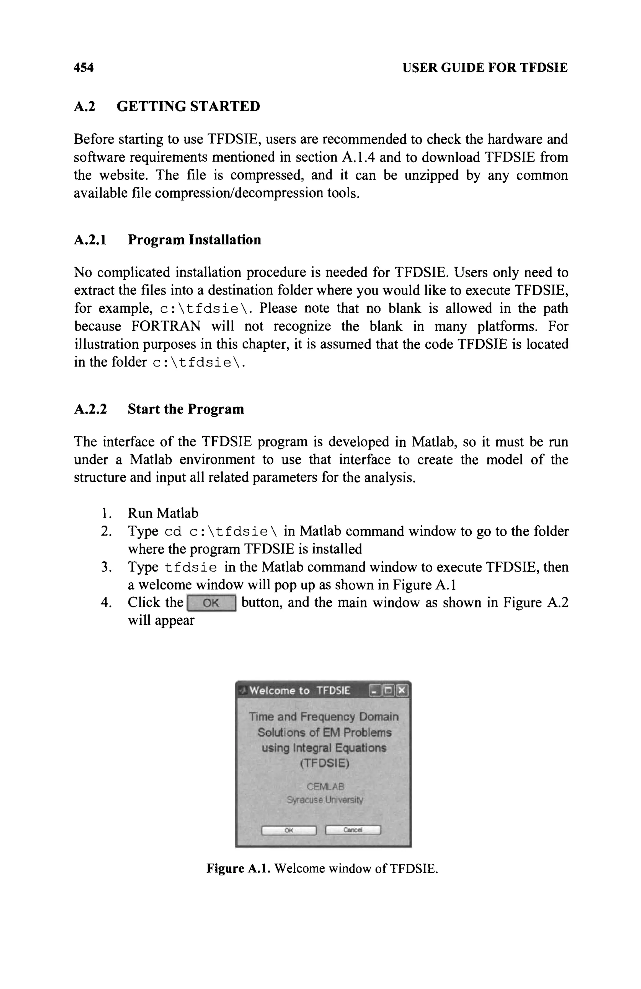
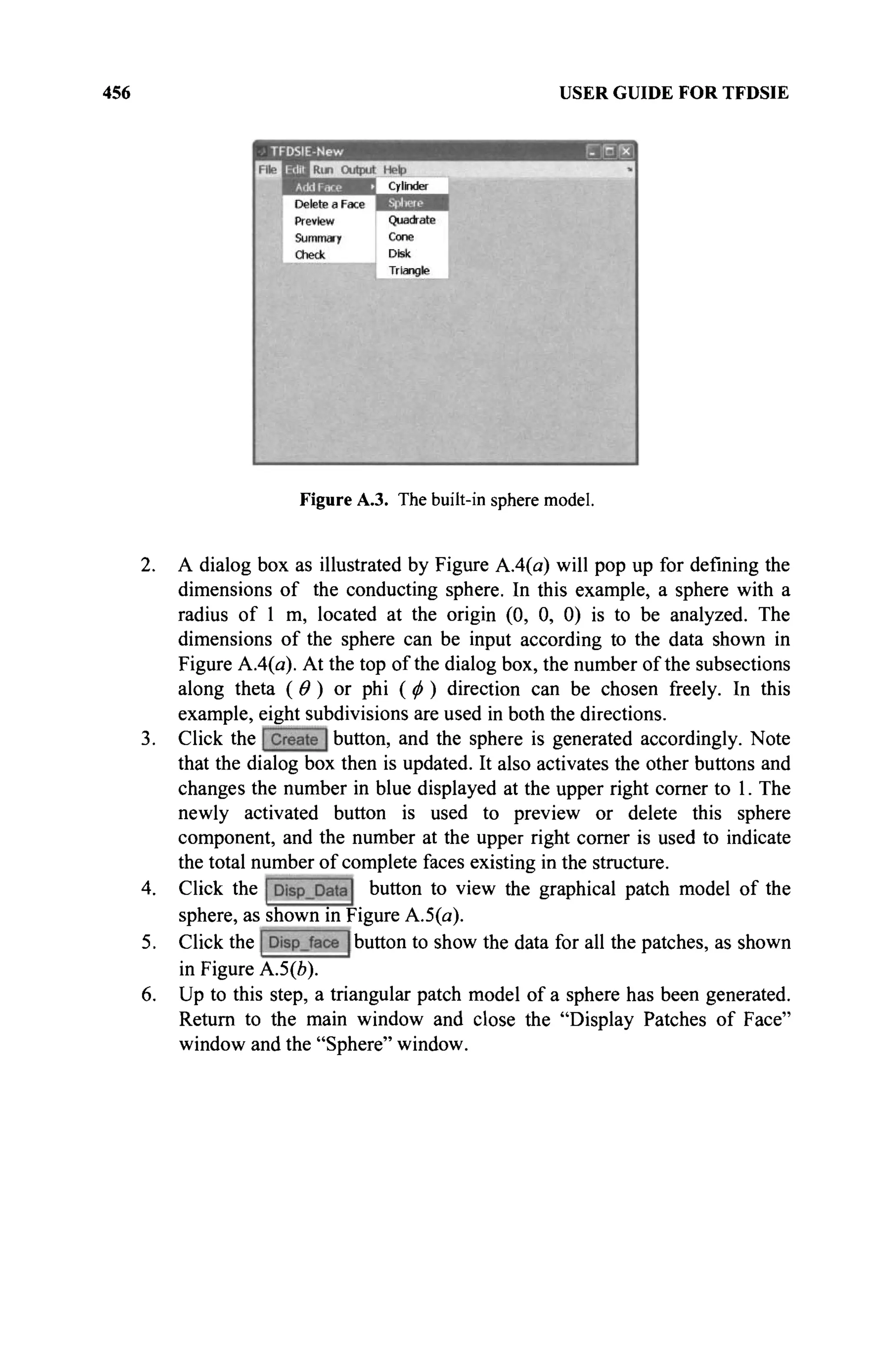
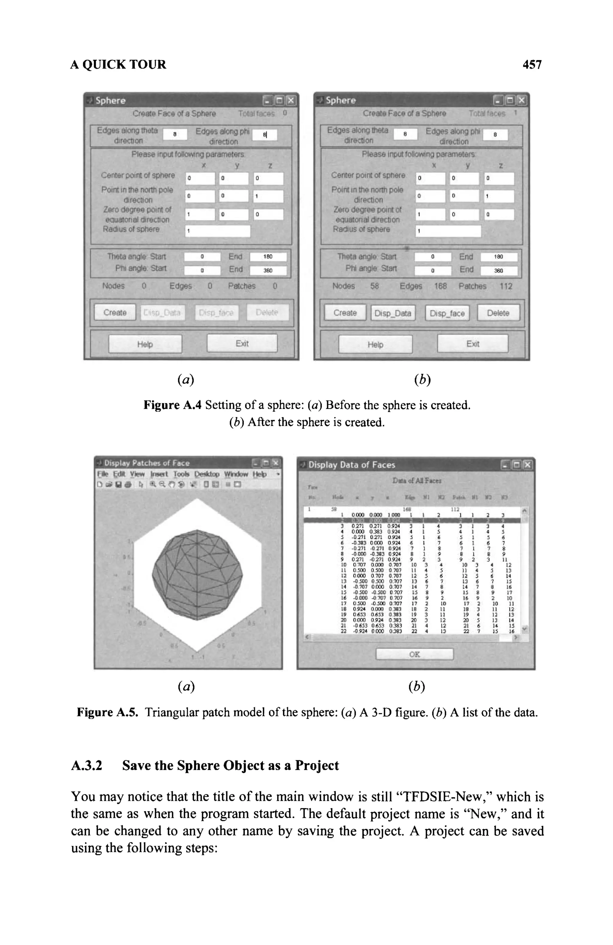
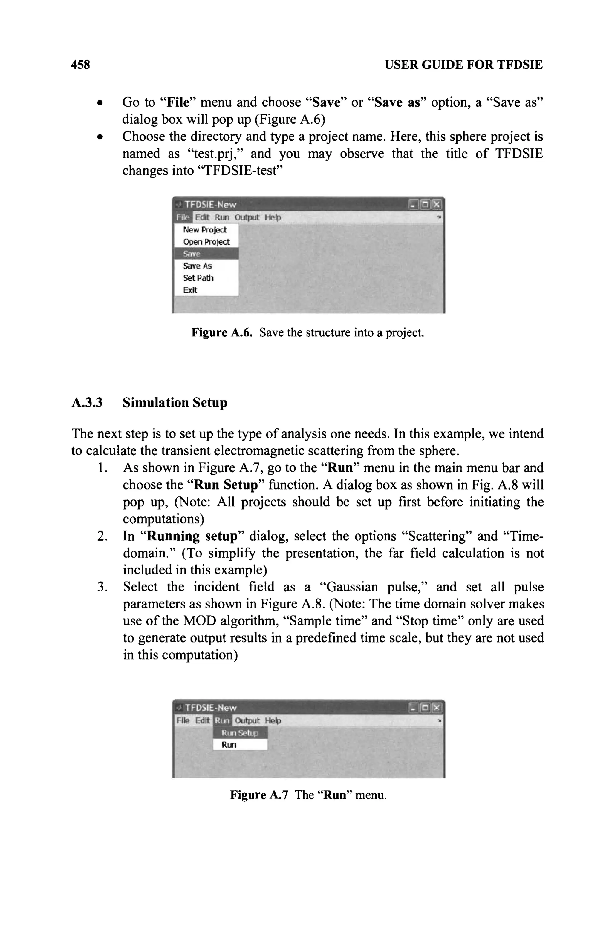
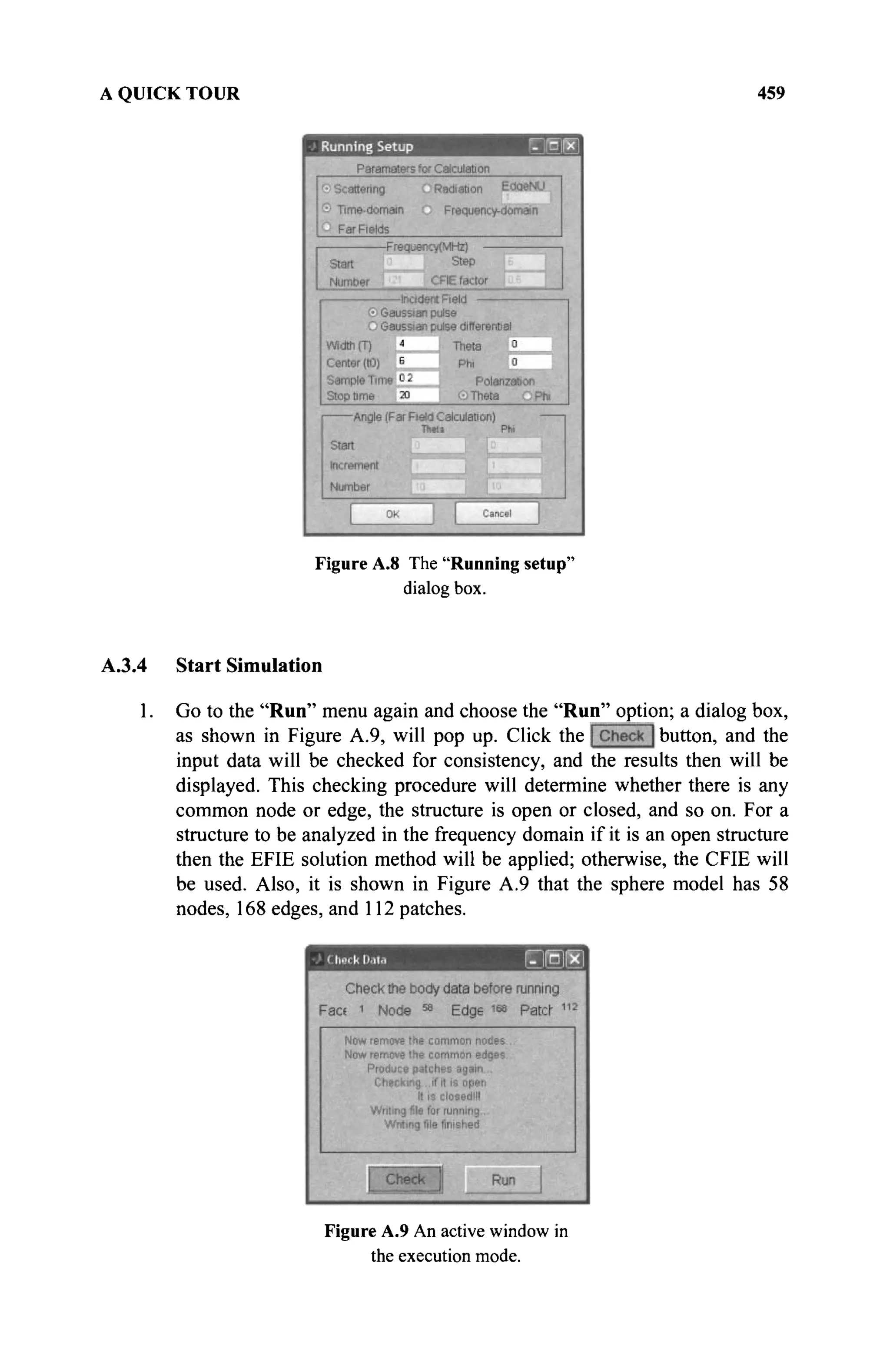
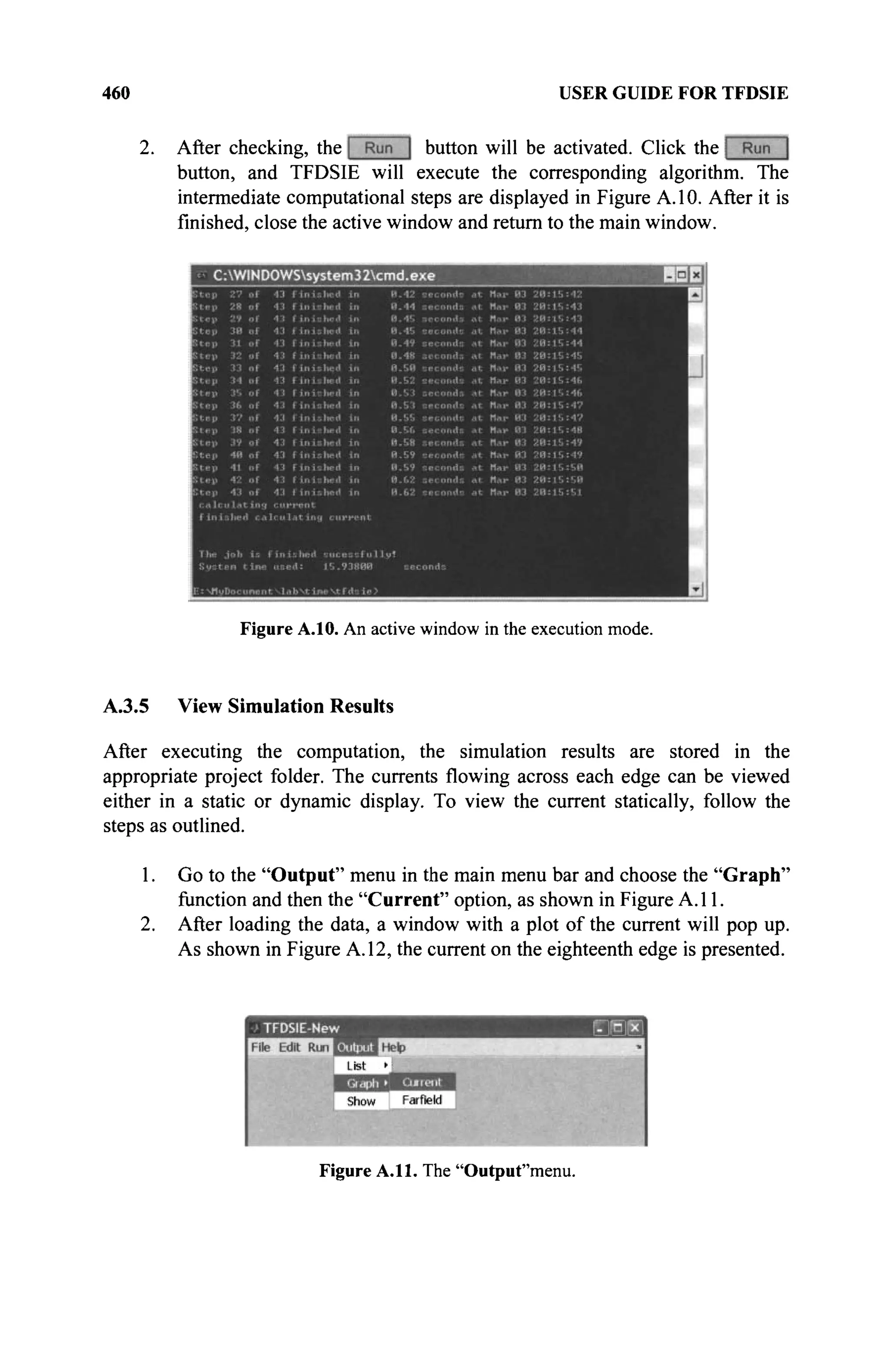
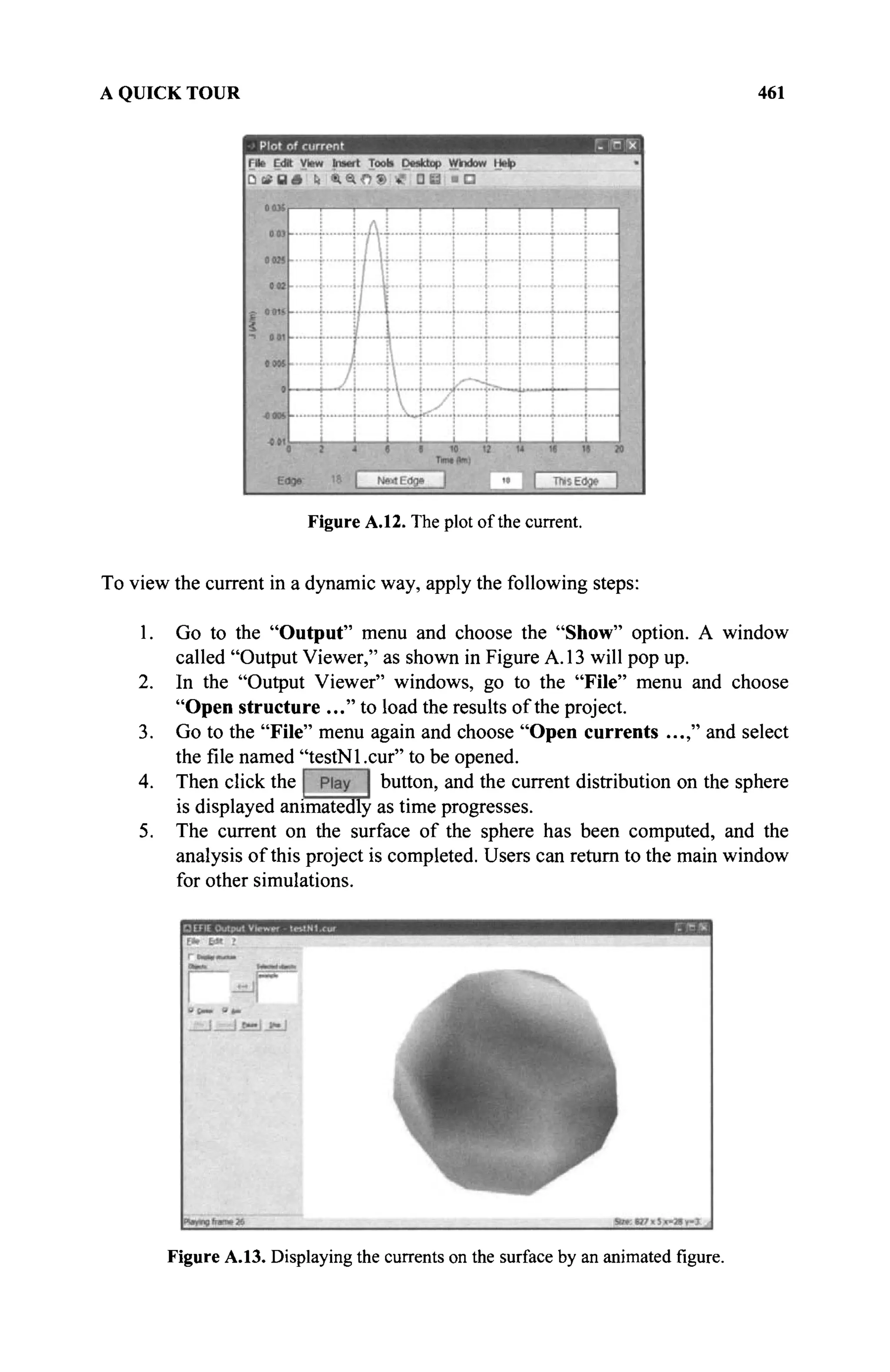
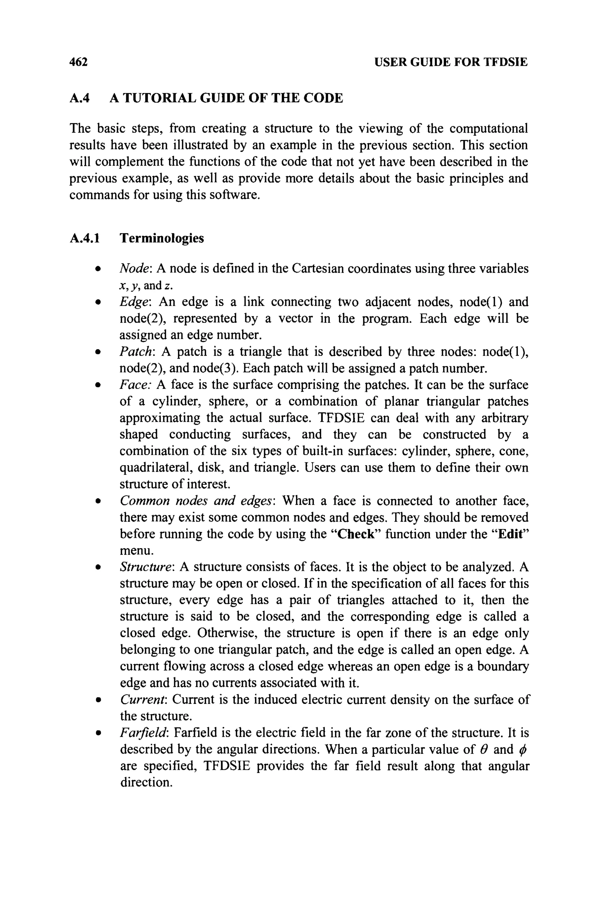
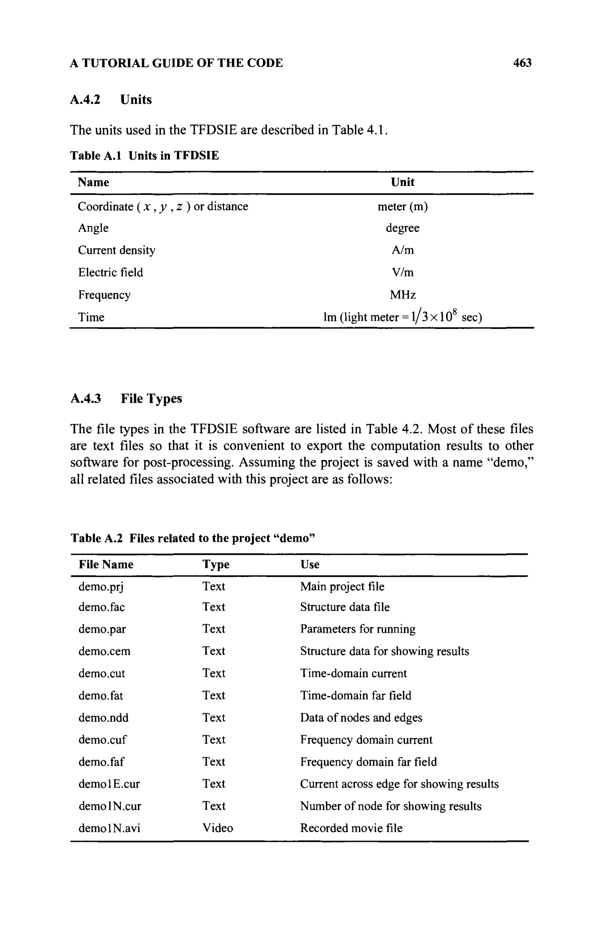
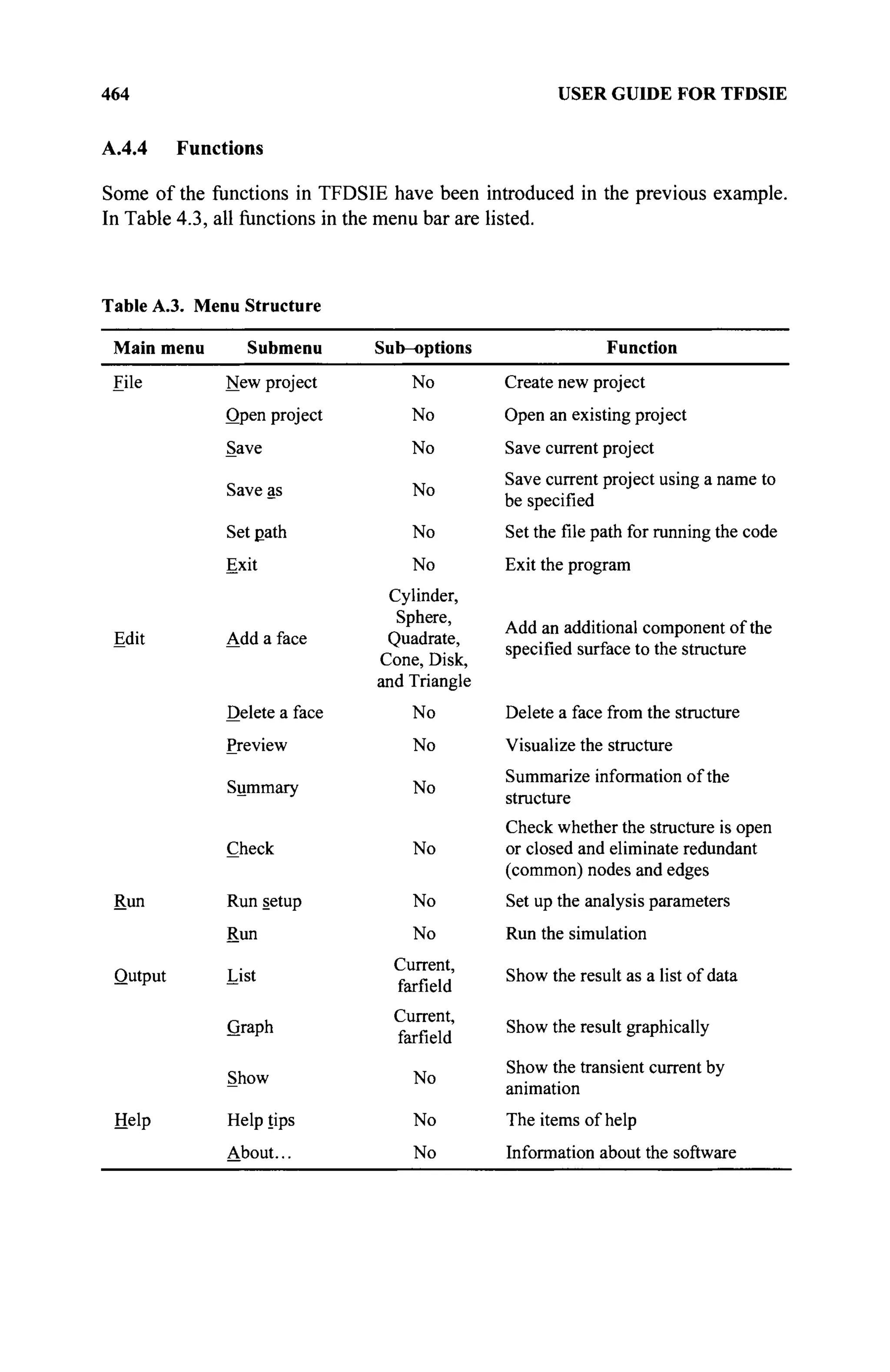
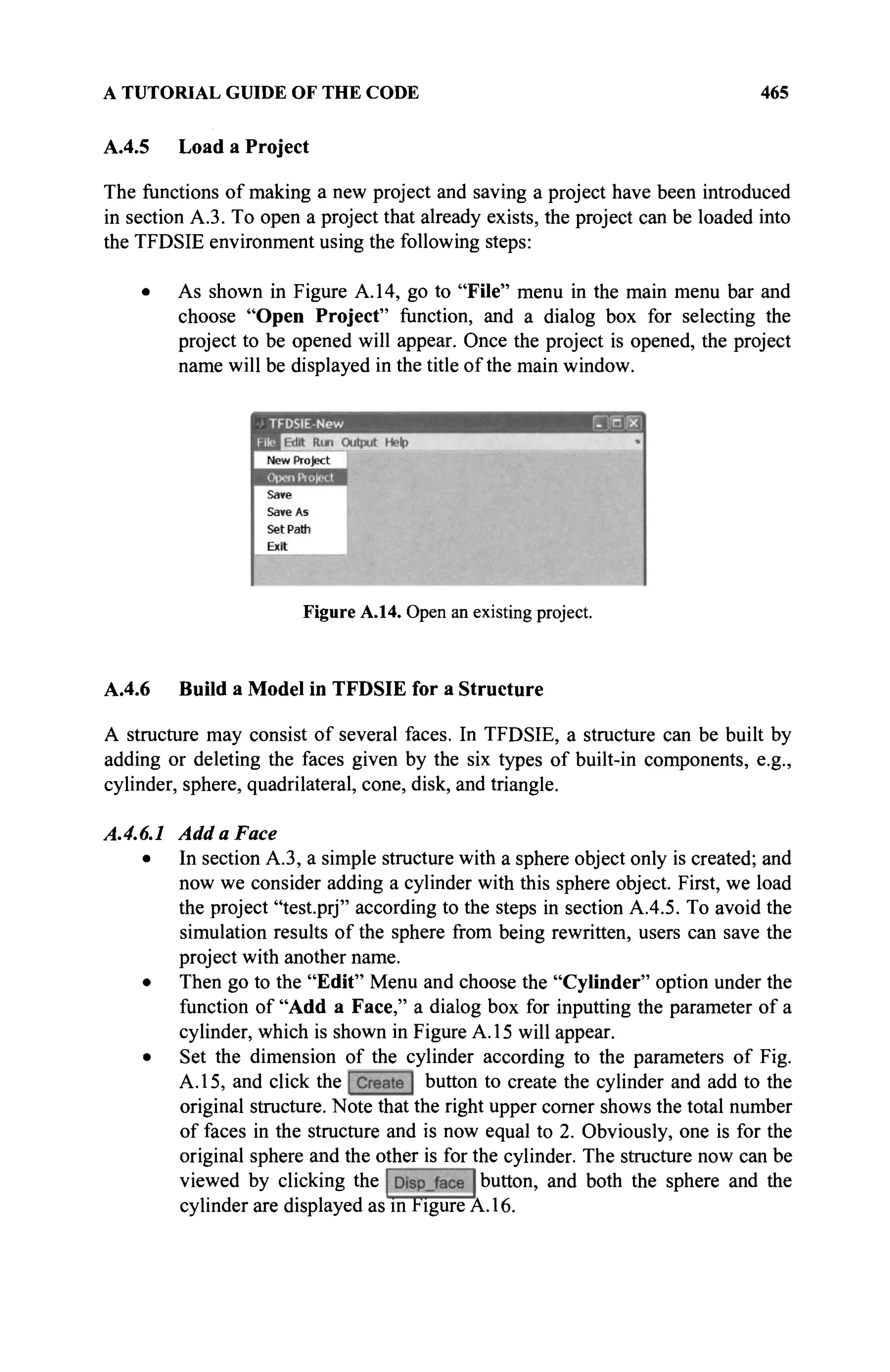
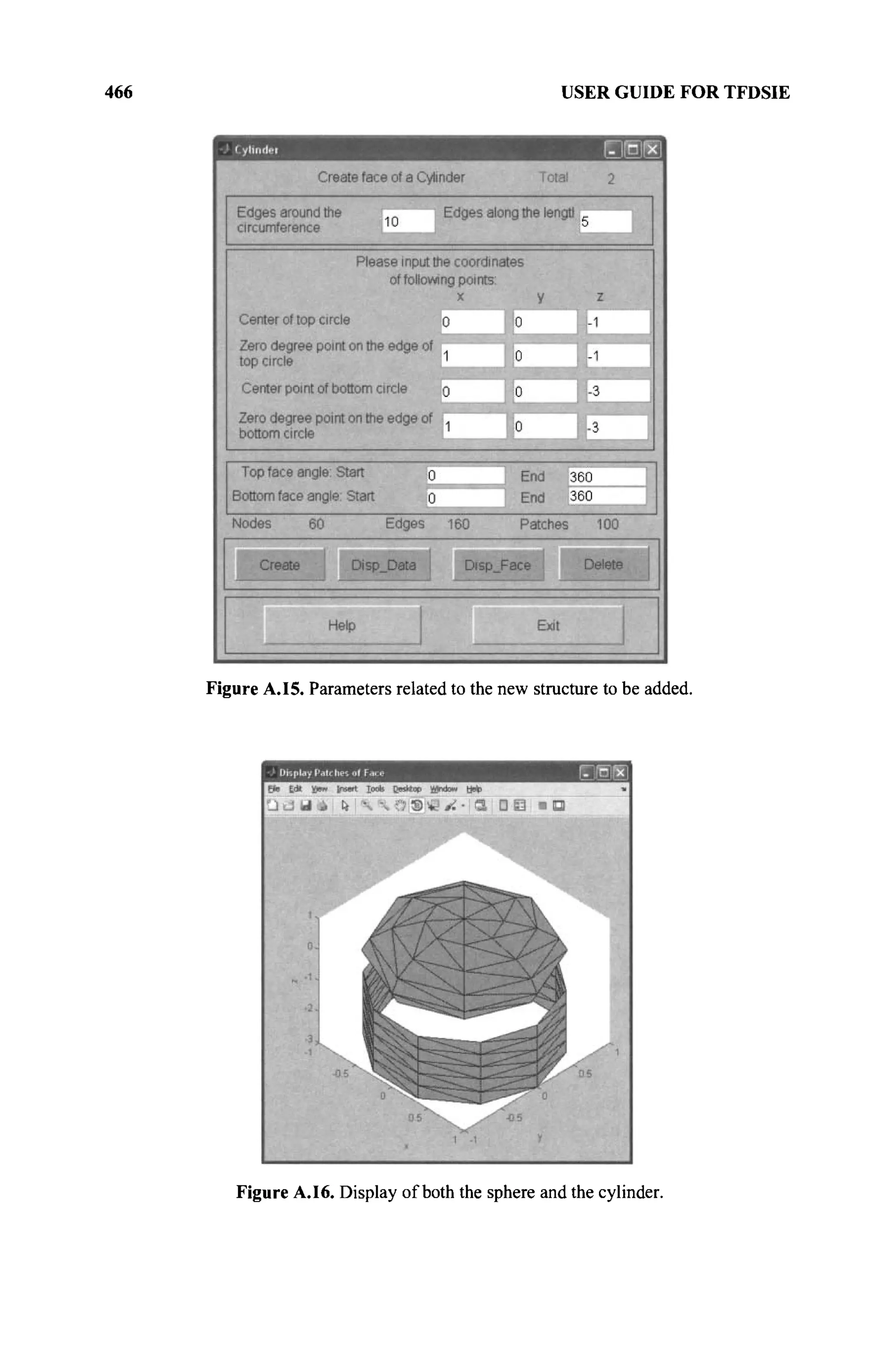
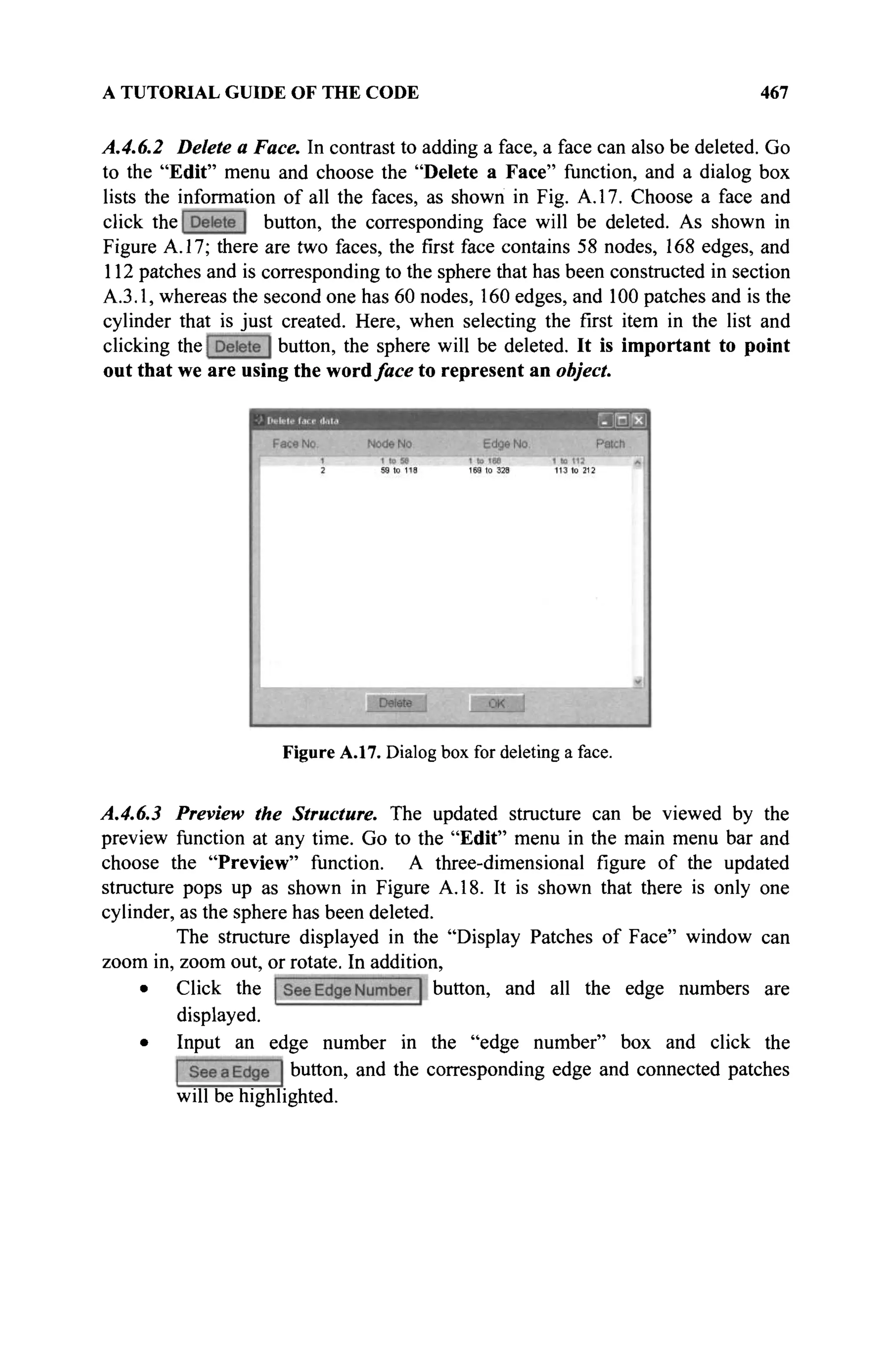
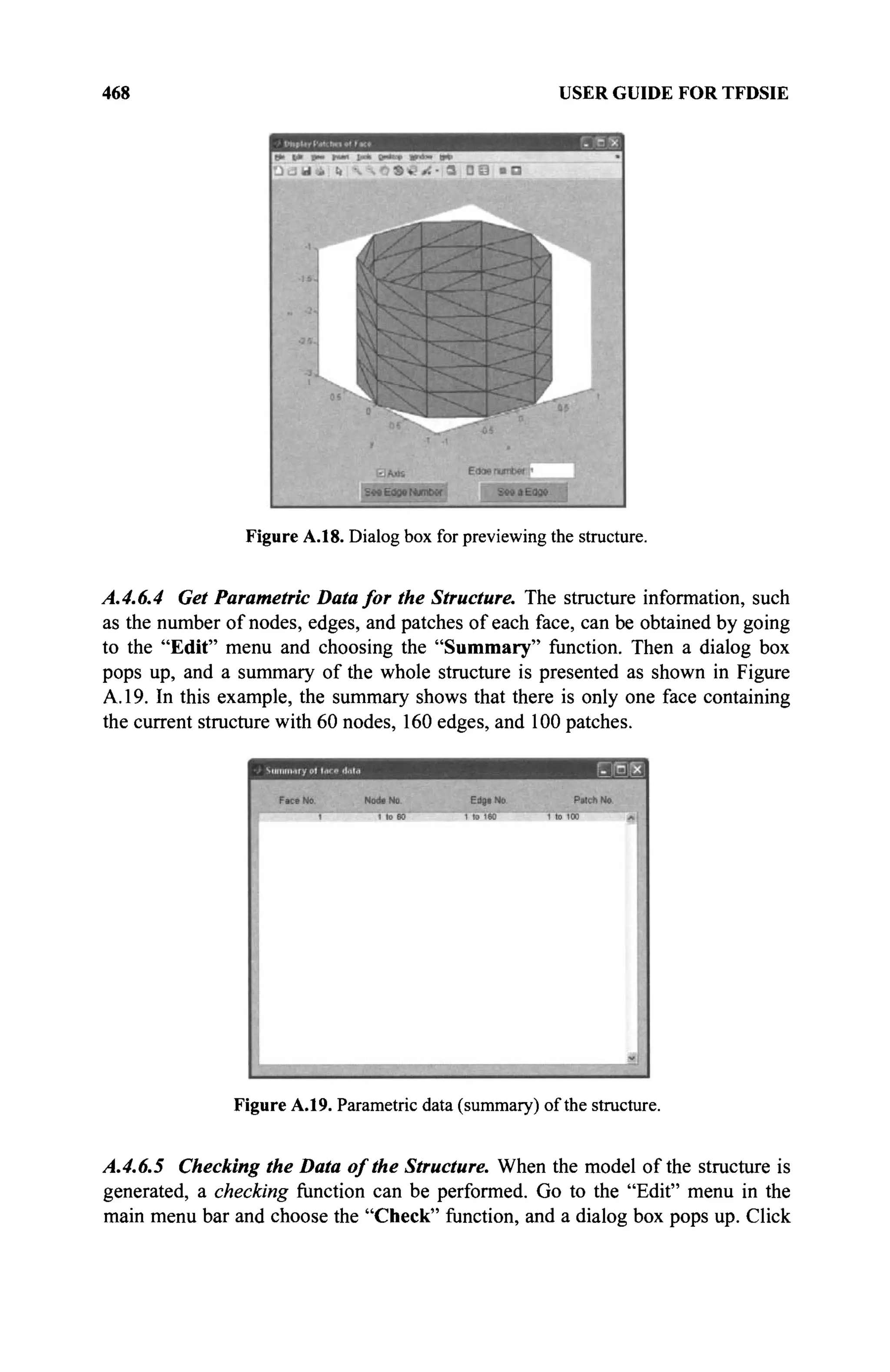
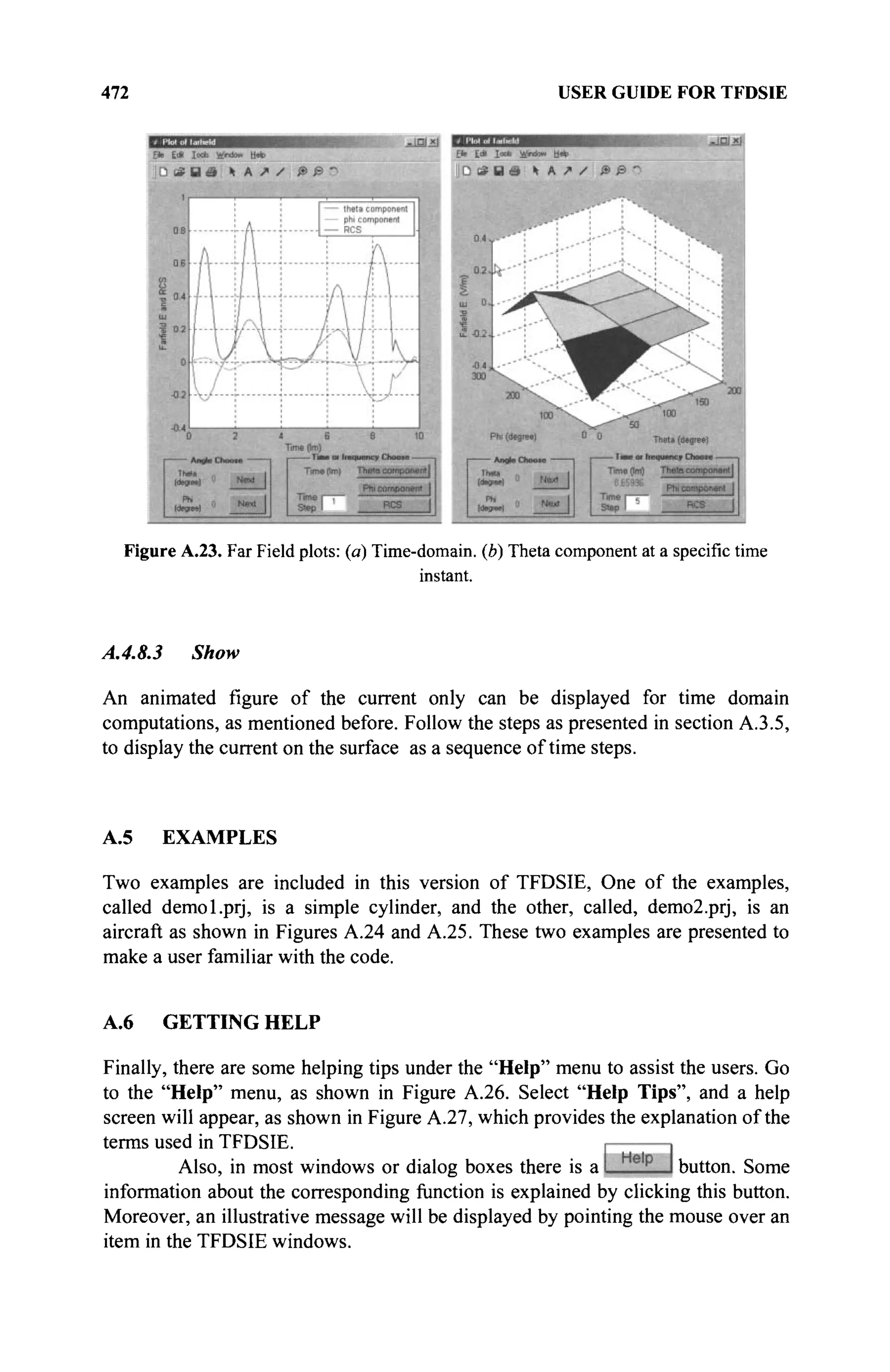
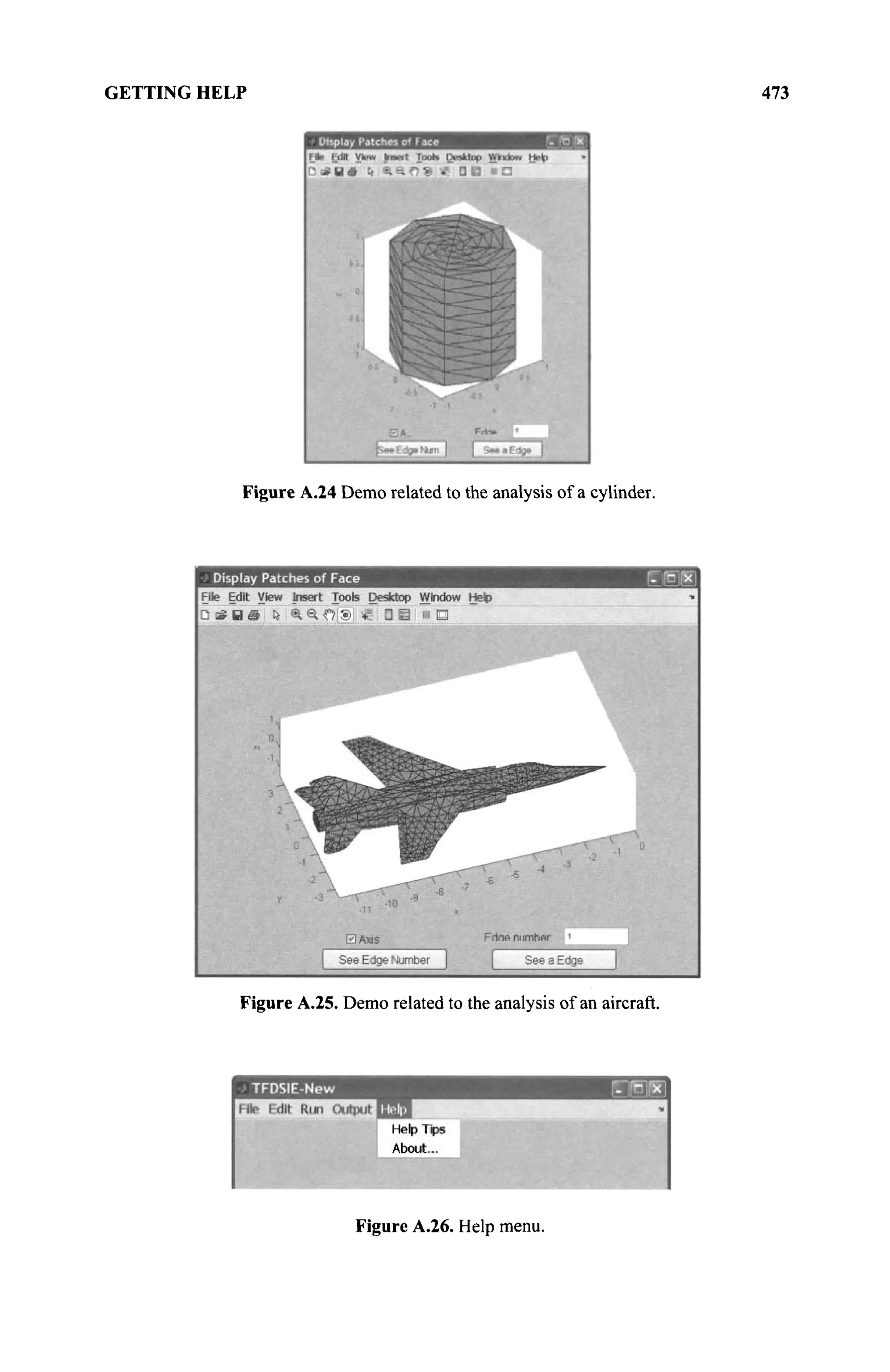
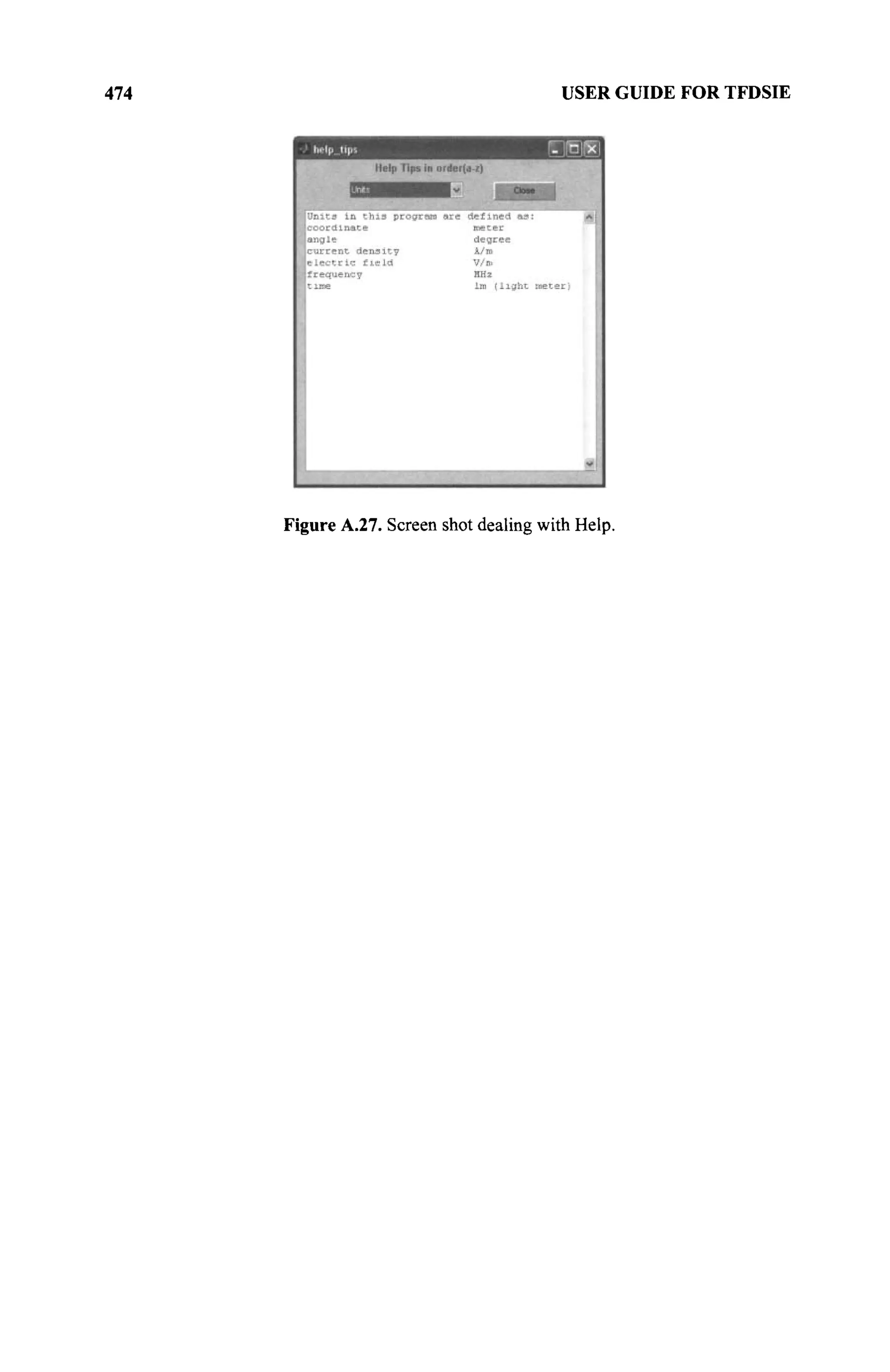
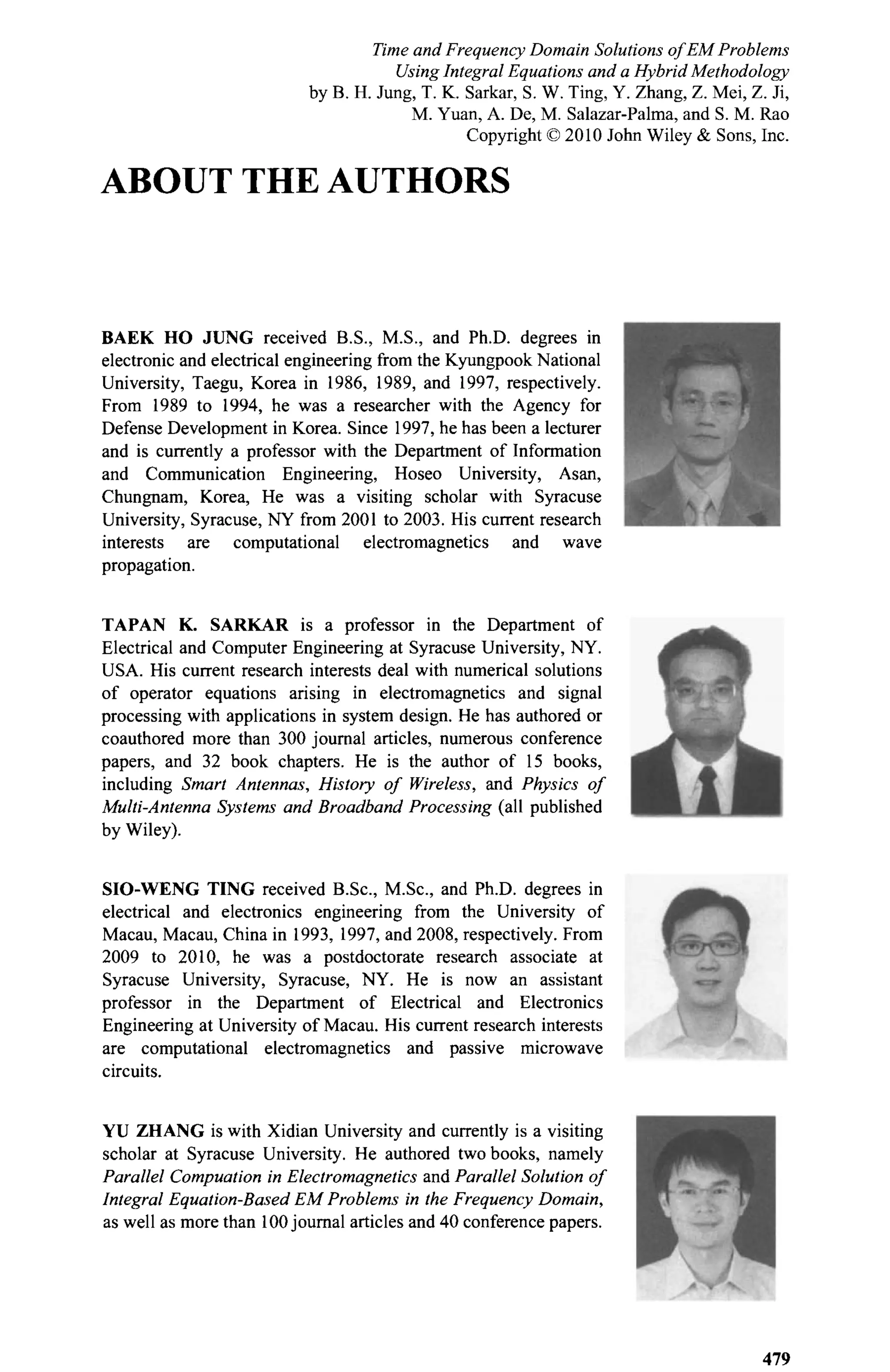
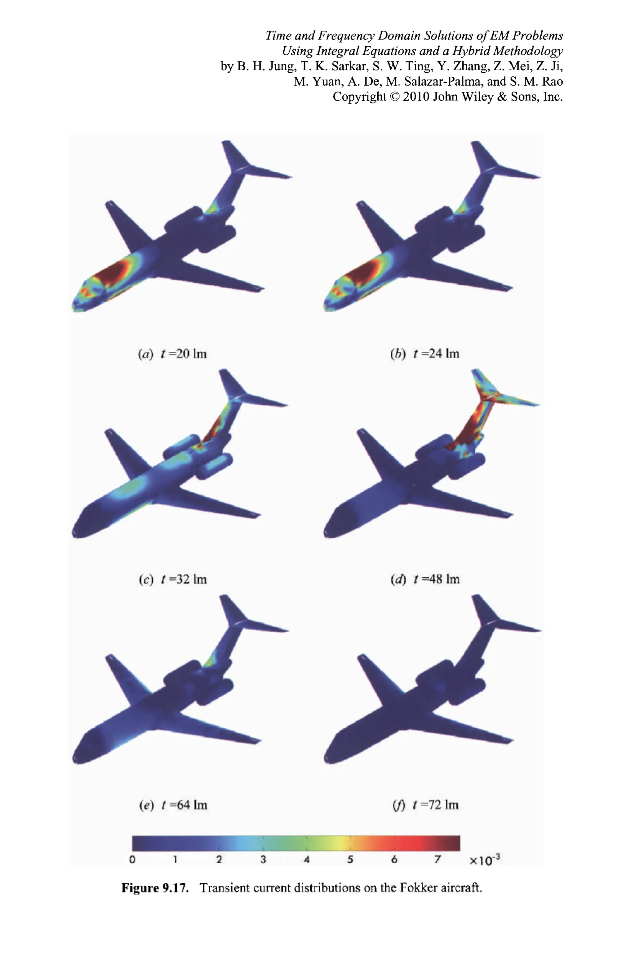
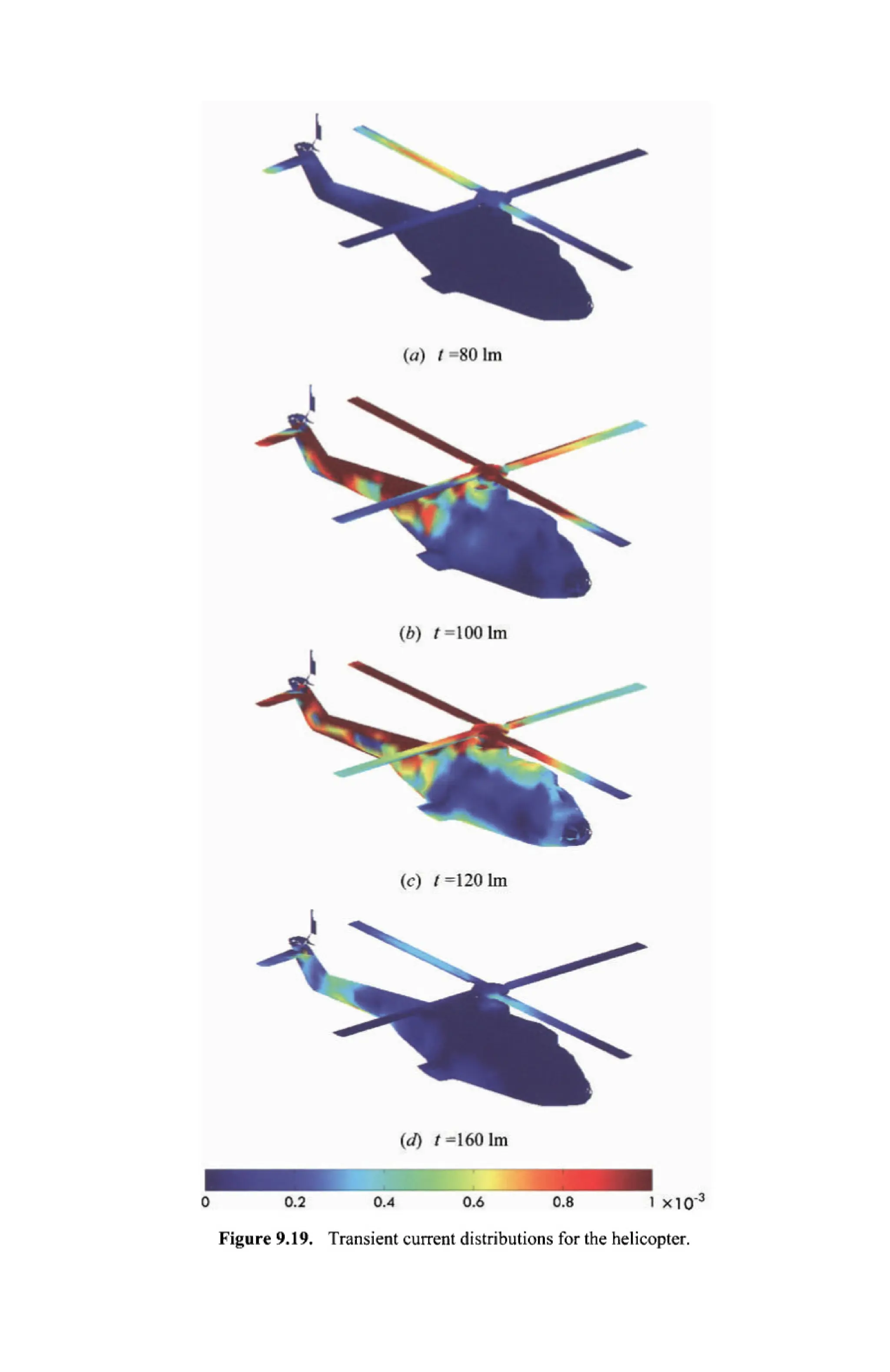
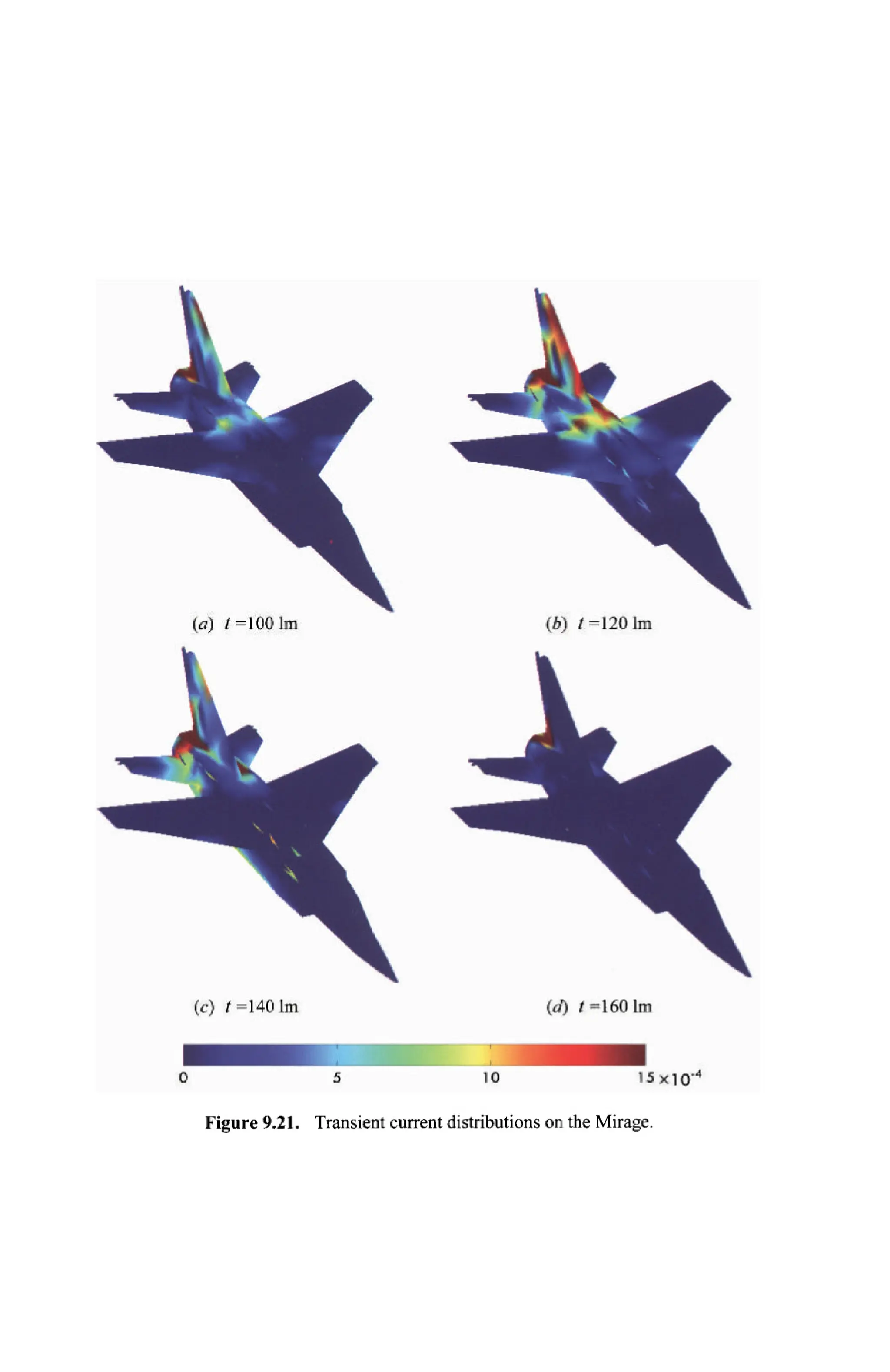
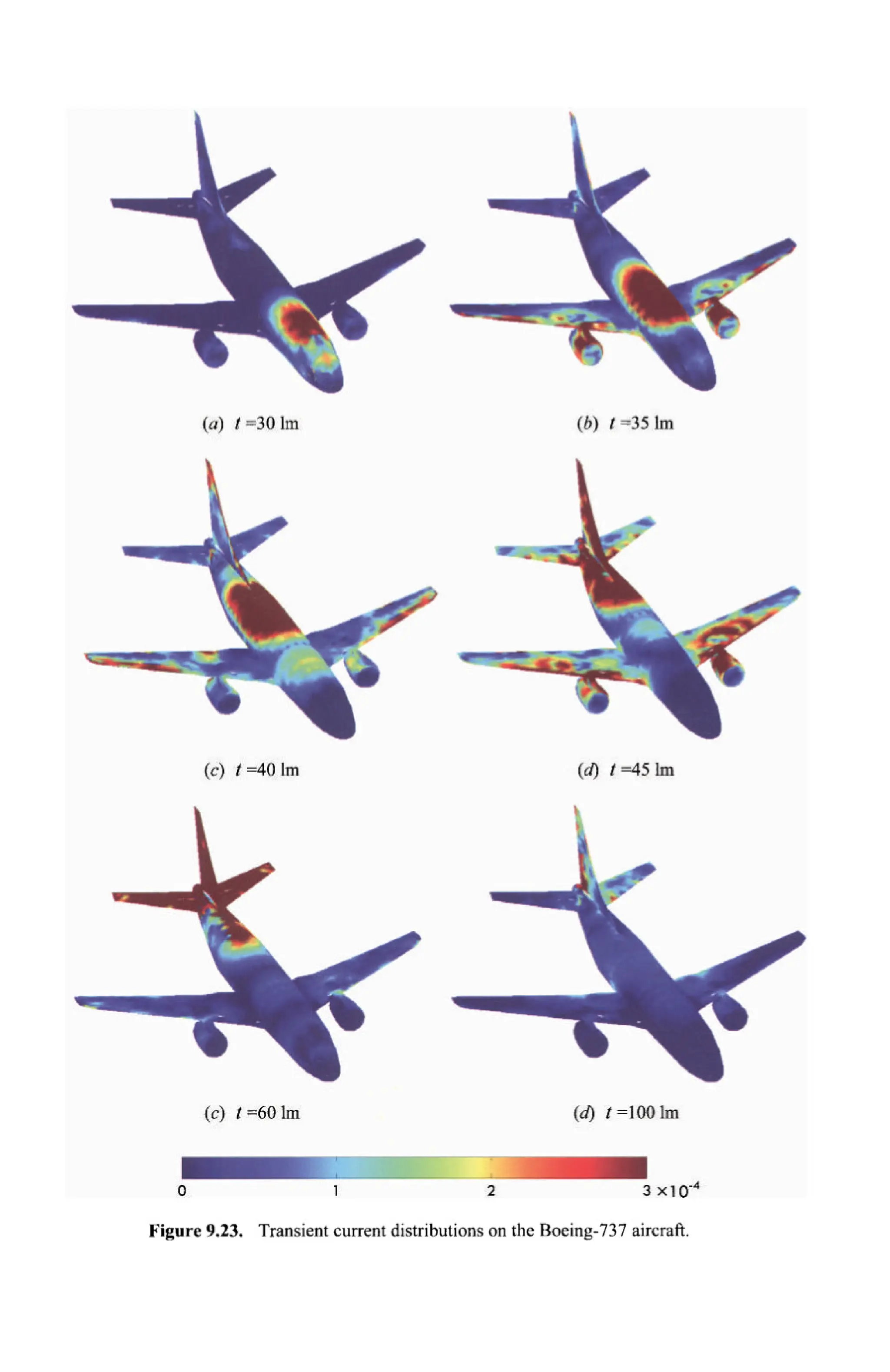


The document is a comprehensive resource on electromagnetic (EM) problems in time and frequency domains utilizing integral equations and hybrid methodologies, edited by Kai Chang. It covers various mathematical methods, numerical solutions, and practical applications related to conducting structures, dielectric objects, and composite materials. The text is published under the Wiley series in Microwave and Optical Engineering and includes extensive references and numerical examples.


![4.[29 34]signal integrity analysis of modified coplanar waveguide structure u...](https://cdn.slidesharecdn.com/ss_thumbnails/4-29-34signalintegrityanalysisofmodifiedcoplanarwaveguidestructureusingadi-fdtdmethod-111203185017-phpapp01-thumbnail.jpg?width=640&height=640&fit=bounds)


