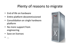
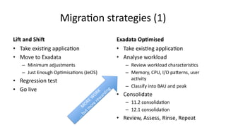
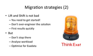
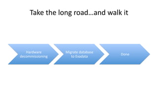
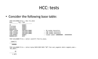
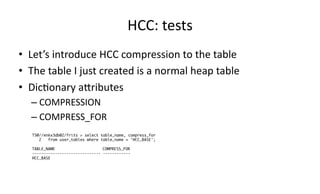
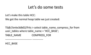
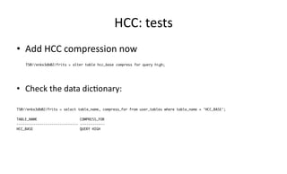
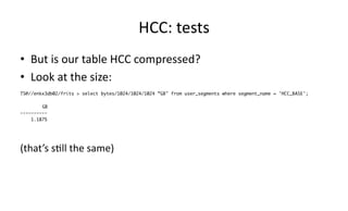
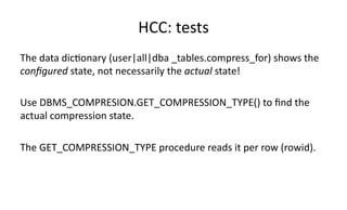
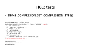
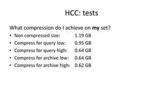
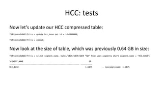
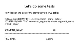
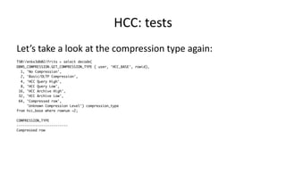
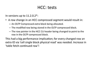
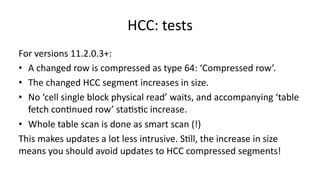
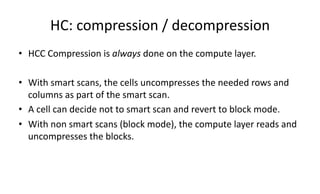
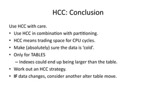
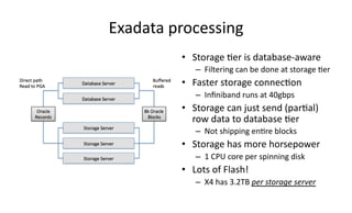
1. Think
Exa!
Learning
what
you
need
to
learn
about
Exadata
Forge5ng
some
of
what
we
thought
important
2.
3. Who
We
Are
• Oracle-centric Consulting Partner focusing on the Oracle Technology
Stack
• Exadata Specialized Partner status (one of a handful globally)
• 200+ successful Exadata implementations
• Dedicated, in-house Exadata lab (POV, Patch Validation)
• Exadata specific: capacity planning, patching, POC, troubleshooting
• Presence in the US, UK, DE and NL.
• That means we are open for a challenge in NL too!!
10. Plenty
of
reasons
to
migrate
• End
of
life
on
hardware
• En>re
plaGorm
decommissioned
• Consolida>on
on
single
hardware
plaGorm
• No
more
support
from
engineering
• Save
on
licenses
• ...
11. Why
and
where
Exadata
can
work
• Shared
infrastructure
– Sharing
your
storage
with
everyone
is
not
efficient
– Sketchy
I/O
performance
• Old
hardware
– End
of
life
for
your
system
• Consolida>on
– You
are
consolida>ng
databases
12. Where
you
might
come
from
All
logos/trademarks
belong
to
their
righGul
owners
13. Migra>on
strategies
(1)
Li:
and
Shi:
• Take
exis>ng
applica>on
• Move
to
Exadata
– Minimum
adjustments
– Just
Enough
Op>misa>ons
(JeOS)
• Regression
test
• Go
live
Exadata
Op=mised
• Take
exis>ng
applica>on
• Analyse
workload
– Review
workload
characteris>cs
– Memory,
CPU,
I/O
paXerns,
user
ac>vity
– Classify
into
BAU
and
peak
• Consolidate
– 11.2
consolida>on
– 12.1
consolida>on
• Review,
Assess,
Rinse,
Repeat
14. Migra>on
strategies
(2)
• Li[
and
Shi[
is
not
bad
– You
need
to
get
started!
– Don’t
over-‐engineer
the
solu>on
– First
results
quickly
• But
– Don’t
stop
there
– Analyse
workload
– Op>mise
for
Exadata
Think Exa!!
15. What
you
would
miss
• If
you
don’t
inves>gate
in
understanding
Exadata
– …
you
don’t
learn
about
Smart
I/O
and
– More
specifically
Smart
Scans
– You
miss
out
on
the
use
of
Hybrid
Columnar
Compression
– …
and
how
to
use
it
most
efficiently
– …
you
don’t
get
to
use
I/O
Resource
Manager
• And
we
forgot
to
men>on
all
the
other
useful
features!
19. Take
the
long
road…and
walk
it
Hardware
decommissioning
Migrate
database
to
Exadata
Done
20. Take
the
long
road…and
walk
it
Hardware
decommissioning
Migrate
database
to
Exadata
Simplify,
op>mise,
21. Common
scenario
• Highly
visible
applica>on
moving
to
Exadata
– Lots
of
TB
of
old,
cold,
historic
data
– Mixed
workload:
OLTP
and
Repor>ng
– Database
started
as
7.x
on
Solaris
2.4
– Thousands
of
data
files
due
to
UFS
limita>ons
• No
one
dares
to
touch
it
• Killed
with
hardware
in
the
past
– Run
out
of
more
powerful
hardware
to
kill
problem
with
22. How
to
migrate?
• Endianness
conversion
needed
– Source
PlaGorm
is
Big
Endian
– Exadata
is
Linux
=
LiXle
Endian
• This
takes
>me
• “The
Best
Way”
to
migrate
depends
on
your
environment
– Many
use
a
combina>on
of
TTS
and
Replica>on
23. One
way
to
migrate
NFS
export
Logical
replica>on
Old
live
system
1.
Convert
datafiles
2.
Apply
transac>ons
24. Think
Exa!
• You
s>ll
have
thousands
of
data
files
– All
of
which
are
2
GB
in
size
– Think
about
backup
>me
• You
are
not
using
Exadata
features
yet
– Simplify
– Op>mise
• Consider
using
bigfile
tablespaces
• Time
to
convert
to
locally
managed
tablespaces
:)
27. Concepts
guide
2
Tables
and
Table
Clusters,
Hybrid
Columnar
Compression
With
Hybrid
Columnar
Compression,
the
database
stores
the
same
column
for
a
group
of
rows
together.
The
data
block
does
not
store
data
in
row-‐major
format,
but
uses
a
combina>on
of
both
row
and
columnar
methods.
Storing
column
data
together,
with
the
same
data
type
and
similar
characteris>cs,
drama>cally
increases
the
storage
savings
achieved
from
compression.
The
database
compresses
data
manipulated
by
any
SQL
opera>on,
although
compression
levels
are
higher
for
direct
path
loads.
Database
opera>ons
work
transparently
against
compressed
objects,
so
no
applica>on
changes
are
required.
28. Oracle
compression
This
means
HCC
is
radically
different
from
the
other
compression
methods
available
in
Oracle:
• Table
compression
/
OLTP
compression
– Values
are
stored
in
a
symbol
table
per
block,
rows
use
pointer
to
symbol
table.
• Index
compression
– One
or
more
columns
are
stored
in
a
symbol
table
per
block,
“rows”
use
pointer
to
symbol
table.
• These
compression
types
are
essen>ally
deduplica>on.
29. HCC:
tests
• Consider
the
following
base
table:
TS@//enkx3db02/frits > desc hcc_base
Name Null Type
------------ ---- --------------
ID NUMBER
CLUSTERED NUMBER
SCATTERED NUMBER
RANDOMIZED NUMBER
SHORT_STRING VARCHAR2(4000) -- 30 random characters
LONG_STRING1 VARCHAR2(4000) -- 130 random characters
LONG_STRING2 VARCHAR2(4000) -- 130 random characters
LONG_NUMBER NUMBER -- random number 1000000000 - 9999999999
RANDOM_DATE DATE
TS@//enkx3db02/frits > select count(*) from hcc_base;
COUNT(*)
----------
3000000
TS@//enkx3db02/frits > select bytes/1024/1024/1024 “GB” from user_segments where segment_name =
'HCC_BASE';
GB
----------
1.1875
30. HCC:
tests
• Let’s
introduce
HCC
compression
to
the
table
• The
table
I
just
created
is
a
normal
heap
table
• Dic>onary
aXributes
– COMPRESSION
– COMPRESS_FOR
TS@//enkx3db02/frits > select table_name, compress_for
2 from user_tables where table_name = 'HCC_BASE';
TABLE_NAME COMPRESS_FOR
------------------------------ ------------
HCC_BASE
31. Let’s
do
some
tests
Let’s
make
this
table
HCC:
We
got
the
normal
heap
table
we
just
created:
TS@//enkx3db02/frits
>
select
table_name,
compress_for
from
user_tables
where
table_name
=
'HCC_BASE';
TABLE_NAME
COMPRESS_FOR
-‐-‐-‐-‐-‐-‐-‐-‐-‐-‐-‐-‐-‐-‐-‐-‐-‐-‐-‐-‐-‐-‐-‐-‐-‐-‐-‐-‐-‐-‐
-‐-‐-‐-‐-‐-‐-‐-‐-‐-‐-‐-‐
HCC_BASE
32. HCC:
tests
• Add
HCC
compression
now
TS@//enkx3db02/frits > alter table hcc_base compress for query high;
• Check
the
data
dic>onary:
TS@//enkx3db02/frits > select table_name, compress_for from user_tables where table_name = 'HCC_BASE';
TABLE_NAME COMPRESS_FOR
------------------------------ ------------
HCC_BASE QUERY HIGH
33. HCC:
tests
• But
is
our
table
HCC
compressed?
• Look
at
the
size:
TS@//enkx3db02/frits > select bytes/1024/1024/1024 ”GB" from user_segments where segment_name = 'HCC_BASE';
GB
----------
1.1875
(that’s
s>ll
the
same)
34. HCC:
tests
The
data
dic>onary
(user|all|dba
_tables.compress_for)
shows
the
configured
state,
not
necessarily
the
actual
state!
Use
DBMS_COMPRESION.GET_COMPRESSION_TYPE()
to
find
the
actual
compression
state.
The
GET_COMPRESSION_TYPE
procedure
reads
it
per
row
(rowid).
36. HCC:
tests
Actually,
if
an
HCC
mode
is
set
on
a
table,
a
direct
path
insert
method
(kcbl*
code)
is
needed
in
order
to
make
the
rows
HCC
compressed.
This
is
not
en>rely
uncommon,
basic
compression
works
the
same
way.
37. HCC:
tests
Direct
path
inserts
methods
include:
-‐ Insert
/*+
append
*/
-‐ Create
table
as
select
-‐ Parallel
DML
-‐ SQL*loader
direct
path
loads
-‐ Alter
table
move
-‐ Online
table
redefini>on
38. HCC:
tests
Now
we
got
an
HCC
mode
set
on
this
table,
we
can
use
‘alter
table
move’
to
make
it
truly
HCCed!
TS@//enkx3db02/frits > alter table hcc_base move;
Let’s
look
at
the
size
again:
TS@//enkx3db02/frits > select bytes/1024/1024/1024 ”GB" from user_segments where segment_name = 'HCC_BASE';
GB
----------
0.640625 -- was 1.1875
39. HCC:
tests
Actually,
this
can
be
done
in
one
go:
TS@//enkx3db02/frits > alter table hcc_base move compress for query high;
Now
let’s
look
with
DBMS_COMPRESSION.GET_COMPRESSION_TYPE
again:
41. HCC:
tests
What
compression
do
I
achieve
on
my
set?
• Non
compressed
size:
1.19
GB
• Compress
for
query
low:
0.95
GB
• Compress
for
query
high:
0.64
GB
• Compress
for
archive
low:
0.64
GB
• Compress
for
archive
high:
0.62
GB
42. HCC:
tests
Now
let’s
update
our
HCC
compressed
table:
TS@//enkx3db02/frits > update hcc_base set id = id+1000000;
TS@//enkx3db02/frits > commit;
Now
look
at
the
size
of
table,
which
was
previously
0.64
GB
in
size:
TS@//enkx3db02/frits > select segment_name, bytes/1024/1024/1024 ”GB" from user_segments where segment_name = 'HCC_BASE';
SEGMENT_NAME GB
------------------------------------------------------------ ----------
HCC_BASE 1.6875 -- noncompressed: 1.1875
43. Let’s
do
some
tests
Now
look
at
the
size
of
my
previously
0,64
GB
table:
TS@//enkx3db02/frits
>
select
segment_name,
bytes/
1024/1024/1024
"Gb"
from
user_segments
where
segment_name
=
'HCC_BASE';
SEGMENT_NAME
Gb
-‐-‐-‐-‐-‐-‐-‐-‐-‐-‐-‐-‐-‐-‐-‐-‐-‐-‐-‐-‐-‐-‐-‐-‐-‐-‐-‐-‐-‐-‐-‐-‐-‐-‐-‐-‐-‐-‐-‐-‐-‐-‐-‐-‐-‐-‐-‐-‐-‐-‐-‐-‐-‐-‐-‐-‐-‐-‐-‐-‐-‐-‐-‐-‐-‐-‐-‐-‐-‐-‐-‐-‐-‐-‐-‐-‐-‐-‐-‐-‐-‐
-‐-‐-‐-‐-‐-‐-‐-‐-‐-‐
HCC_BASE
1.6875
44. HCC:
tests
Let’s
take
a
look
at
the
compression
type
again:
TS@//enkx3db02/frits > select decode(
DBMS_COMPRESSION.GET_COMPRESSION_TYPE ( user, 'HCC_BASE', rowid),
1, 'No Compression',
2, 'Basic/OLTP Compression',
4, 'HCC Query High',
8, 'HCC Query Low',
16, 'HCC Archive High',
32, 'HCC Archive Low',
64, 'Compressed row',
'Unknown Compression Level') compression_type
from hcc_base where rownum <2;
COMPRESSION_TYPE
-------------------------
Compressed row
45. HCC:
tests
In
versions
up
to
11.2.0.2*:
• A
row
change
in
an
HCC
compressed
segment
would
result
in:
– An
OLTP
Compressed
extra
block
being
allocated.
– The
modified
row
being
stored
in
the
OLTP
compressed
block.
– The
row
pointer
in
the
HCC
CU
header
being
changed
to
point
to
the
row
in
the
OLTP
compressed
block.
This
had
a
big
performance
implica>on;
for
every
changed
row
an
extra
IO
via
‘cell
single
block
physical
read’
was
needed.
Increase
in
‘table
fetch
con>nued
row’!
46. HCC:
tests
For
versions
11.2.0.3+:
• A
changed
row
is
compressed
as
type
64:
‘Compressed
row’.
• The
changed
HCC
segment
increases
in
size.
• No
‘cell
single
block
physical
read’
waits,
and
accompanying
‘table
fetch
con>nued
row’
sta>s>c
increase.
• Whole
table
scan
is
done
as
smart
scan
(!)
This
makes
updates
a
lot
less
intrusive.
S>ll,
the
increase
in
size
means
you
should
avoid
updates
to
HCC
compressed
segments!
47. HC:
compression
/
decompression
• HCC
Compression
is
always
done
on
the
compute
layer.
• With
smart
scans,
the
cells
uncompresses
the
needed
rows
and
columns
as
part
of
the
smart
scan.
• A
cell
can
decide
not
to
smart
scan
and
revert
to
block
mode.
• With
non
smart
scans
(block
mode),
the
compute
layer
reads
and
uncompresses
the
blocks.
48. HCC:
Conclusion
Use
HCC
with
care.
• Use
HCC
in
combina>on
with
par>>oning.
• HCC
means
trading
space
for
CPU
cycles.
• Make
(absolutely)
sure
the
data
is
‘cold’.
• Only
for
TABLES
– Indexes
could
end
up
being
larger
than
the
table.
• Work
out
an
HCC
strategy.
• IF
data
changes,
consider
another
alter
table
move.
51. Exadata
processing
• Storage
>er
is
database-‐aware
– Filtering
can
be
done
at
storage
>er
• Faster
storage
connec>on
– Infiniband
runs
at
40gbps
• Storage
can
just
send
(par>al)
row
data
to
database
>er
– Not
shipping
en>re
blocks
• Storage
has
more
horsepower
– 1
CPU
core
per
spinning
disk
• Lots
of
Flash!
– X4
has
3.2TB
per
storage
server
52. The
buffer
cache
size
• Size
does
maXer
– Warehouse
workloads
benefit
from
small
buffer
cache
– You
need
direct
path
reads
for
smart
scans
• Small
Table
Threshold
• Size
of
the
segment
– Shrinking
SGA
is
ok
for
warehouse
workloads
• Mixed
workload
in
same
database
is
different
story
53. The
ques>on
about
par>>oning
• On
non-‐Exadata
plaGorms
you
tried
to
– Eliminate
as
much
I/O
as
possible
• Star
schema
• Star
transforma>on
• Bitmap
indexes
• Subpar>>ons
• On
Exadata
– Not
such
a
good
idea
– See
why
56. Smart
Scan
Is
Always
BeXer
™
SQL ID: 5yc3hmz41jf3q Plan Hash: 2481424394
select /* sdr_always */ count(1)
from
t1_subpart
call count cpu elapsed disk query current rows
------- ------ -------- ---------- ---------- ---------- ---------- ----------
Parse 1 0.00 0.00 0 0 0 0
Execute 1 0.00 0.00 0 0 0 0
Fetch 2 2.82 10.99 19996 30894 0 1
------- ------ -------- ---------- ---------- ---------- ---------- ----------
total 4 2.82 11.00 19996 30894 0 1
Elapsed times include waiting on following events:
Event waited on Times Max. Wait Total Waited
---------------------------------------- Waited ---------- ------------
library cache lock 1 0.00 0.00
library cache pin 1 0.00 0.00
SQL*Net message to client 2 0.00 0.00
reliable message 4954 0.00 2.96
enq: KO - fast object checkpoint 9902 0.00 1.21
Disk file operations I/O 1 0.00 0.00
cell smart table scan 7936 0.02 4.44
latch: ges resource hash list 3 0.00 0.00
KJC: Wait for msg sends to complete 2 0.00 0.00
SQL*Net message from client 2 0.00 0.00
********************************************************************************
Well,
maybe
not
57. In
this
case,
surely
not
SQL ID: ctp93ksgpr72s Plan Hash: 2481424394
select /* sdr_auto */ count(1)
from
t1_subpart
call count cpu elapsed disk query current rows
------- ------ -------- ---------- ---------- ---------- ---------- ----------
Parse 1 0.00 0.00 0 0 0 0
Execute 1 0.00 0.00 0 0 0 0
Fetch 2 0.11 0.12 0 30894 0 1
------- ------ -------- ---------- ---------- ---------- ---------- ----------
total 4 0.11 0.12 0 30894 0 1
Elapsed times include waiting on following events:
Event waited on Times Max. Wait Total Waited
---------------------------------------- Waited ---------- ------------
SQL*Net message to client 2 0.00 0.00
SQL*Net message from client 2 6.55 6.55
********************************************************************************
58. Think
Exa!
• Smart
Scans
are
great
for
data
retrieval
– Data
processing
<>
data
retrieval
– Data
to
be
retrieved
should
be
large
• Smart
Scans
don’t
help
retrieve
small
amounts
of
data
– Classic
OLTP-‐style
workload
– Refrain
from
se€ng
_serial_direct_read
=
ALWAYS
system-‐wide
59. Think
Exa!
• Run>me
par>>on
pruning
used
to
be
essen>al
– Small
and
smallest
par>>ons
– Index
based
access
paths
– Very
liXle
I/O,
good
response
>me,
happy
user
• Exadata
can
scoop
lots
of
data
effec>vely
– Don’t
stop
par>>oning
your
data
(-‐>
ILM,
performance)
– But
review
the
strategy
62. Drop
indexes?
• Should
you
drop
all
your
indexes,
when
going
to
the
Exadata
plaGorm?
• What
does
an
index
actually
do?
63. Drop
indexes?
• There
are
two
essen>al
methods
to
find
a
certain
row
in
a
table:
– Scan
the
whole
table
from
beginning
to
end
for
row(s)
matching
your
criteria.
–
Look
up
the
rows
you
need
in
an
ordered
subset
of
the
data*,
then
retrieve
the
rows
via
their
rowids.
– Par>>on
pruning
64. Drop
indexes?
• Let’s
take
the
HCC_BASE
table
from
the
HCC
example.
(Uncompressed)
– Table
size:
1.19GB,
number
of
blocks:
155648.
– The
ID
column
contains
a
unique
ID/number.
• Just
like
the
PK
in
a
lot
of
tables.
65. Drop
indexes?
TS@//enkx3db02/frits > select * from hcc_base where id = 1;
Row
source
sta>s>cs
from
sql_trace:
Physical
reads
TABLE ACCESS STORAGE FULL HCC_BASE (cr=149978 pr=149971 pw=0 time=358570 us cost=40848 size=10074560 card=1657)
Consistent
reads
0.36
seconds
66. Drop
indexes?
• Let’s
create
an
index
on
hcc_base.id:
TS@//enkx3db02/frits > create index i_hcc_base on hcc_base ( id );
• It
results
in
an
object
with
the
following
size:
– Index
size:
0.05GB,
number
of
blocks:
7168
67. Drop
indexes?
Row
source
sta>s>cs
from
sql_trace:
And
1
block
read
to
get
the
row
belonging
to
the
id!
TABLE ACCESS BY INDEX ROWID HCC_BASE
(cr=4 pr=0 pw=0 time=15 us cost=4 size=6080 card=1)
INDEX RANGE SCAN I_HCC_BASE
(cr=3 pr=0 pw=0 time=9 us cost=3 size=0 card=1)
3
blocks
read
from
the
index!
(index
root,
branch,
leaf)
Total
>me
needed
is
0.000015
seconds
68. Drop
indexes:
conclusion
• Dropping
all
indexes
on
Exadata
is
a
myth.
– Some
table
constraints
require
an
index
(PK,
unique).
69. Drop
indexes:
conclusion
• However…
– Some>mes
response>me
can
be
improved
by
removing
indexes.
– Almost
always
these
are
unselec>ve
indexes.
• Exadata
has
far
beXer
full
scan
capability
than
average
non-‐
Exadata
plaGorms.
– This
makes
the
point
where
a
full
scan
gives
a
beXer
response>me
different
on
exadata
versus
non-‐exadata.
70. Drop
indexes:
conclusion
• The
CBO
has
no
Exadata
specific
decisions.
– But
we
just
concluded
that
the
dynamics
of
full
scans
are
different
with
Exadata.
• Resolu>on:
Exadata
(specific)
system
stats:
– exec
dbms_stats.gather_system_stats(‘EXADATA’);
– Sets
op>mizer
internal
calculated
MBRC
value
to
128
(instead
of
8),
which
makes
full
scans
“cheaper”.
73. Simplify
• Try
to
make
everything
as
simple
as
possible.
– Do
NOT
use
privilege
separa>on,
unless
explicitly
needed.
– Do
NOT
change
the
compute
node
filesystem
layout.
• Especially
with
the
new
computenodeupdate
script.
– Use
as
less
Oracle
homes
as
possible.
• Only
having
an
home
for
grid
and
one
db
oracle
home
is
actually
common!
– Do
not
apply
the
resecure
step
in
onecommand.
• This
keeps
ssh
keys
among
other
things.
74. Simplify
• Run
exachk
(exacheck)
monthly.
– When
applying
defaults,
less
errors
will
be
detected.
– Exacheck
changes
with
new
insight
and
new
standards
implemented
in
the
O/S
image.
– This
means
a
new
version
of
exacheck
can
come
up
with
new
or
different
checks.
75. Simplify
• Tablespaces
– Use
ASSM
tablespaces.
– Make
the
tablespaces
bigfile
tablespaces.
• There
are
excep>ons
in
specific
cases,
like
much
sessions
using
temp.
– Group
all
data
belonging
together
into
a
single
tablespace.
• Of
course
there
can
be
excep>ons,
if
there
is
a
good
reason.
– Use
autoextent,
limit
tablespaces
if
there’s
need
to.
76. Simplify
• Tablespaces
(con>nued)
– Try
to
reduce
the
number
of
tablespaces
as
much
as
possible.
– Move
the
audit
table
(AUD$)
from
the
SYSTEM
tablespace.
– Use
8
KB
blocksize,
even
with
a
DWH.
• If
you
have
performance
considera>ons,
do
a
POC
to
measure
performance
impact
between
8KB
and
16KB
(32KB?)
blocksizes.