Download as PDF, PPTX
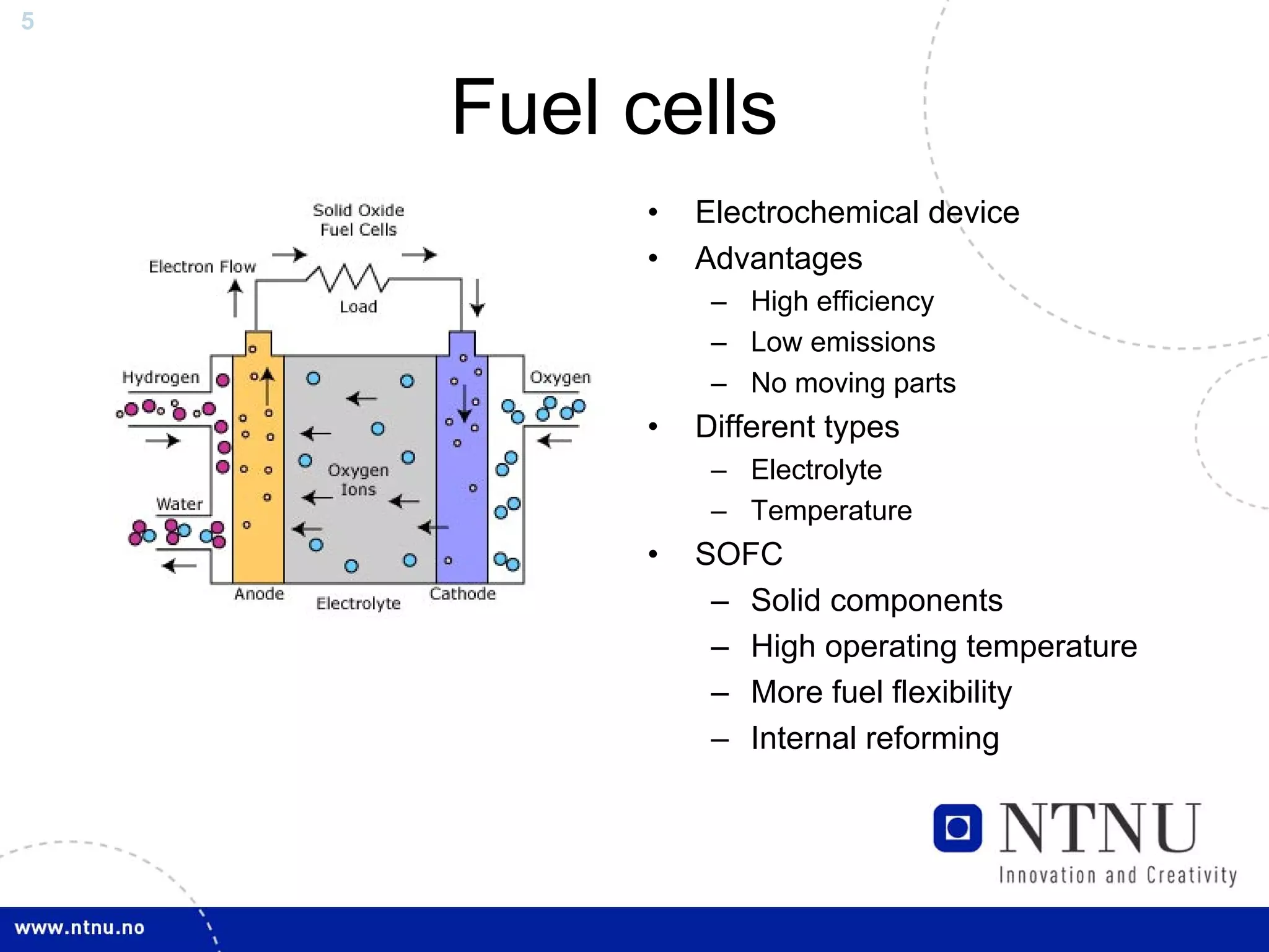
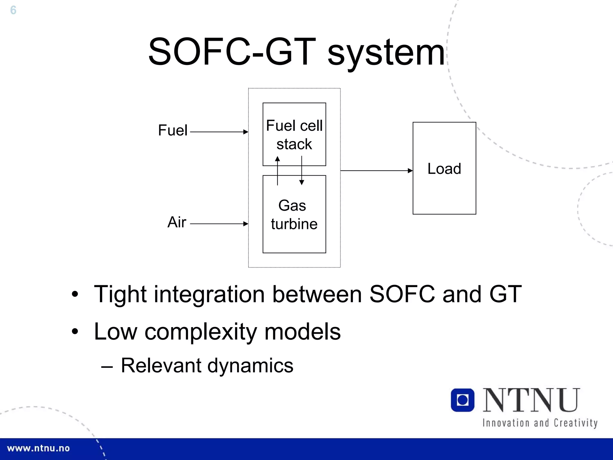
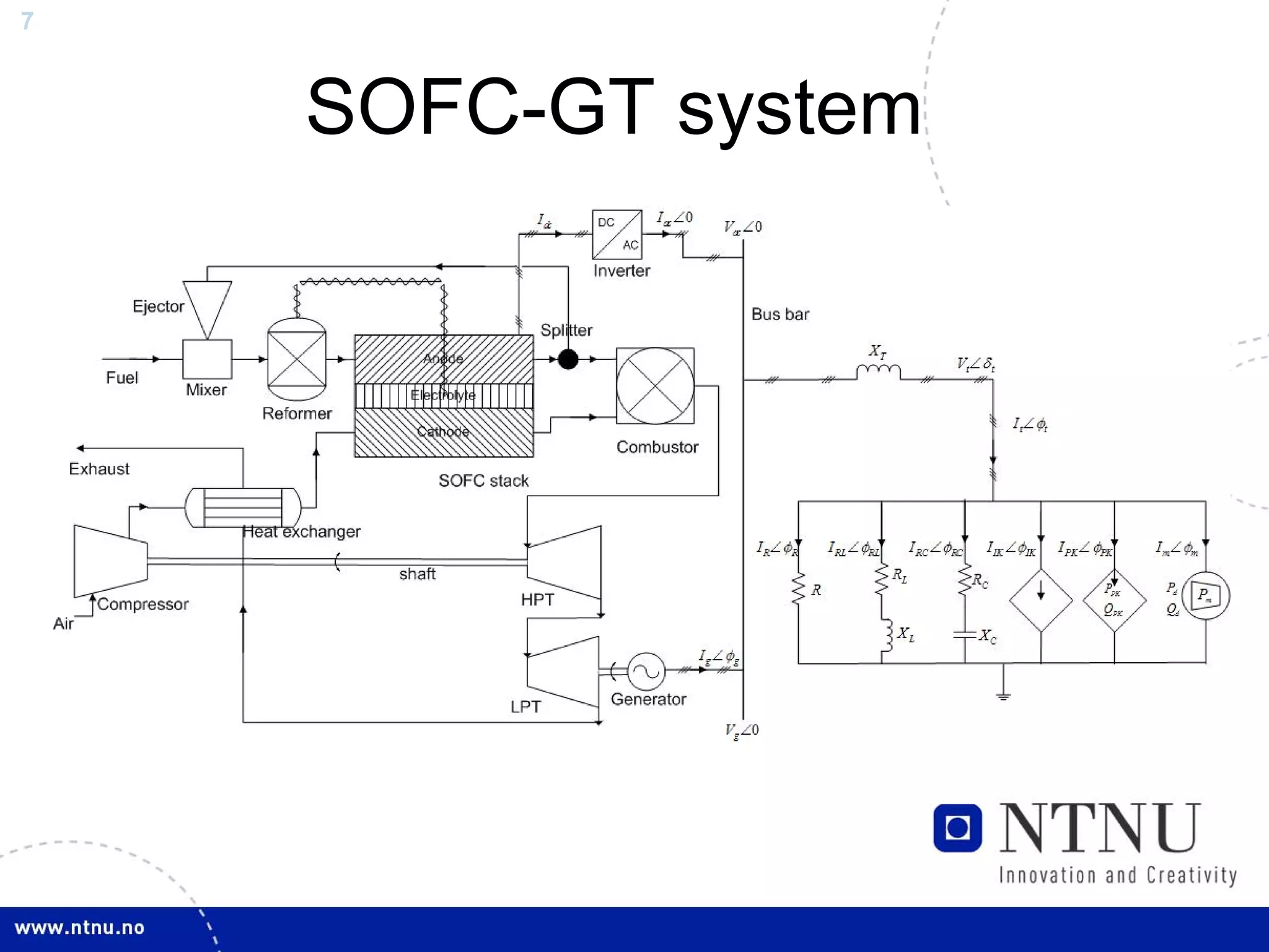
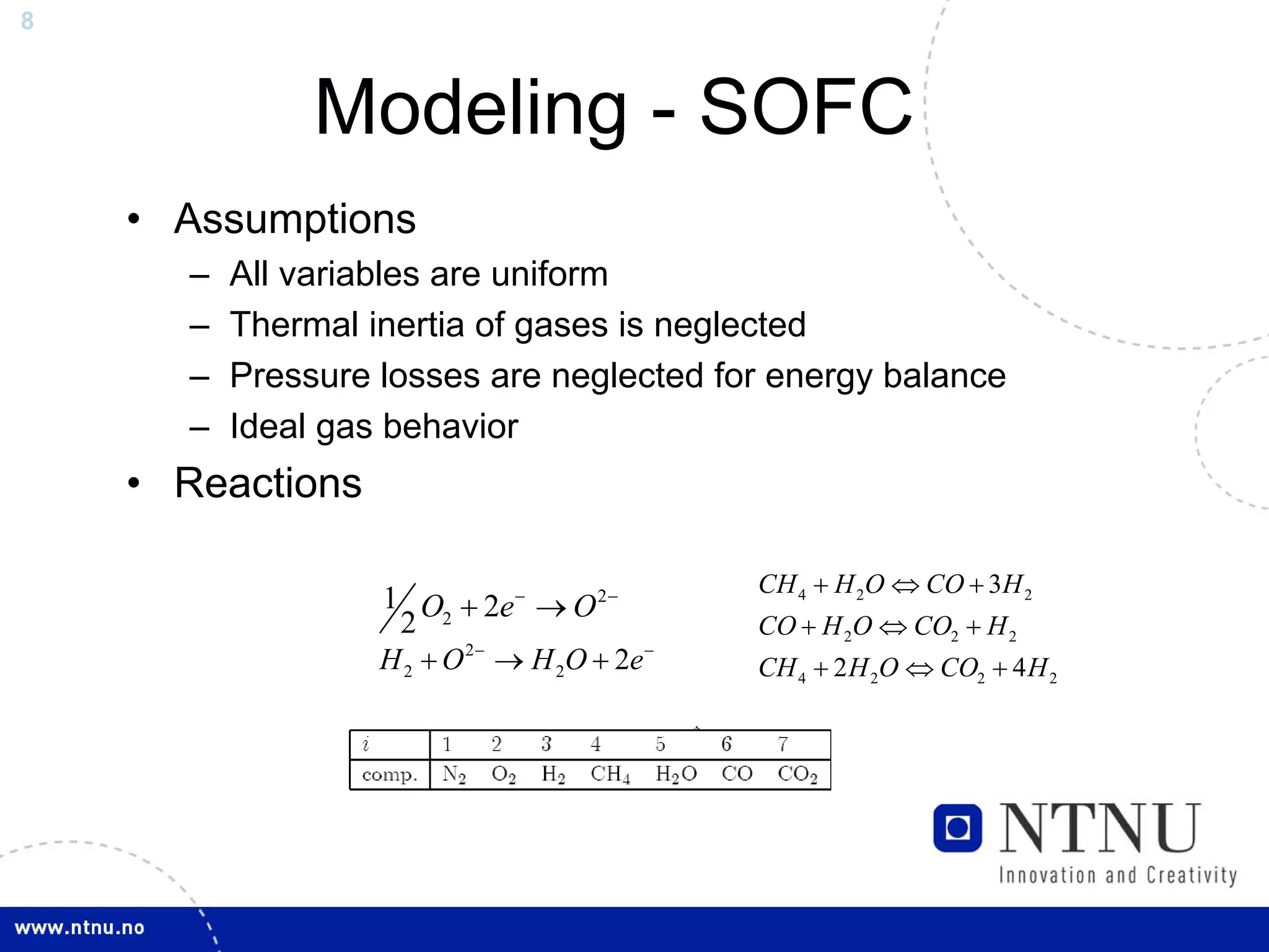
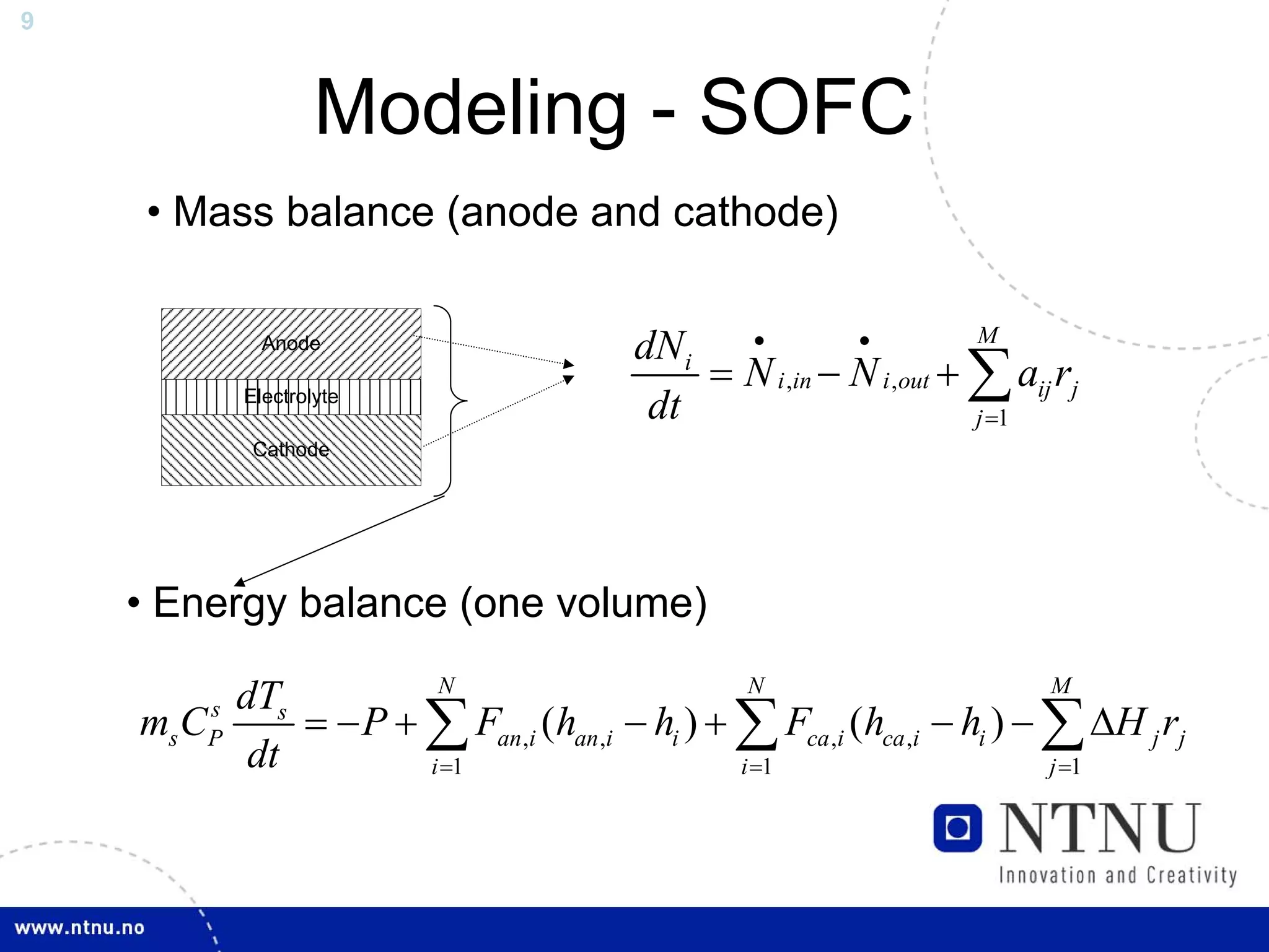
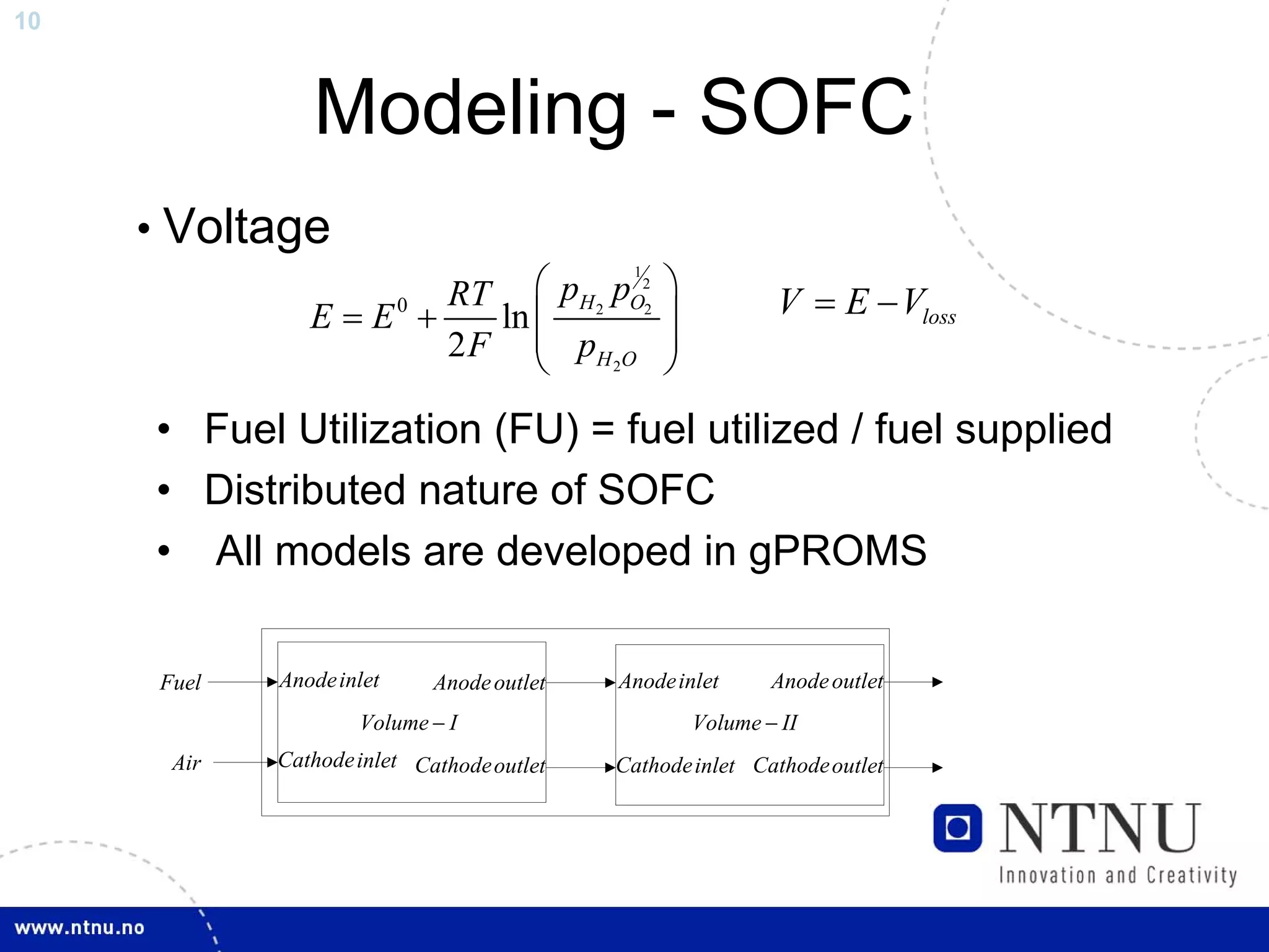
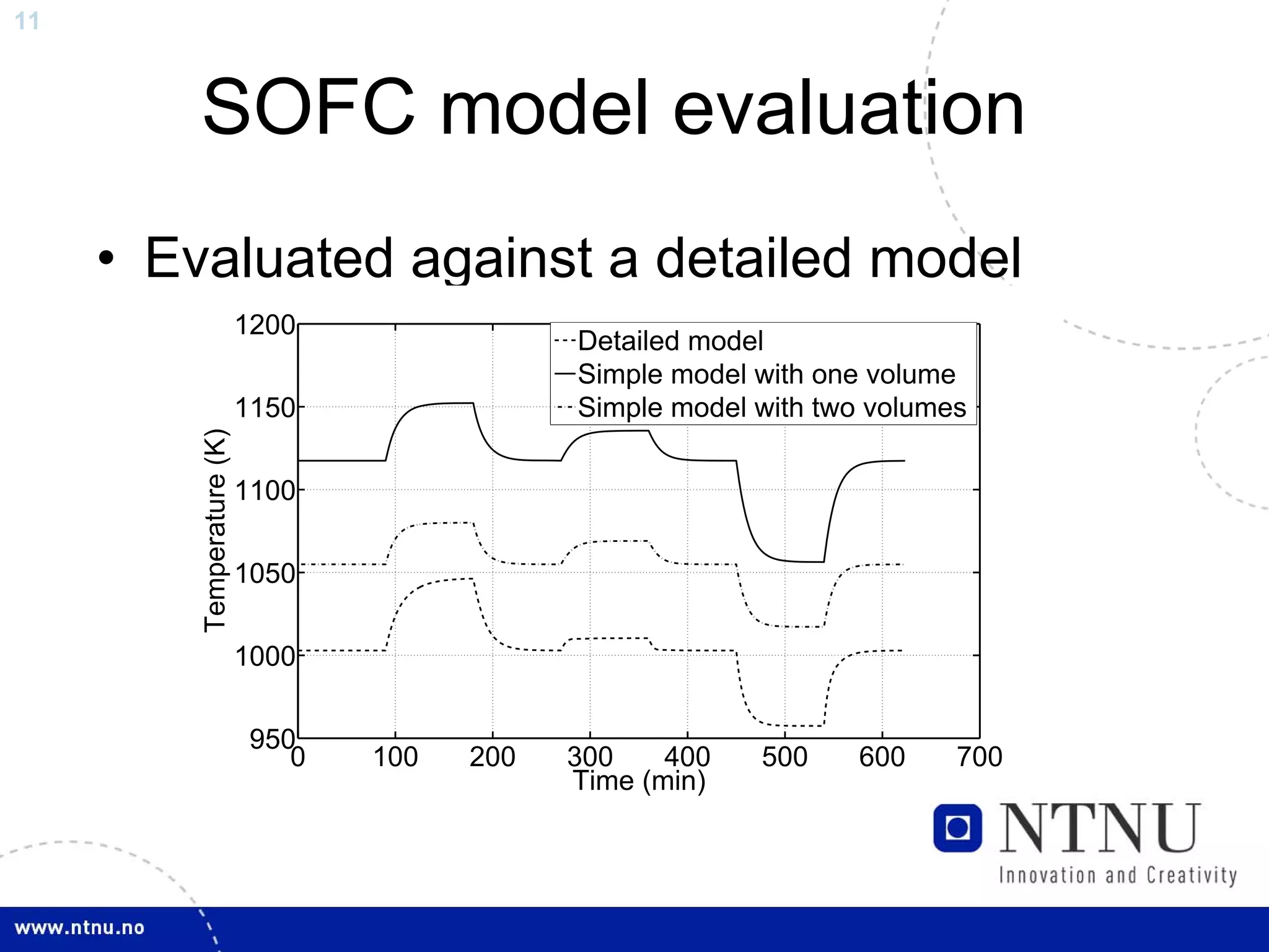
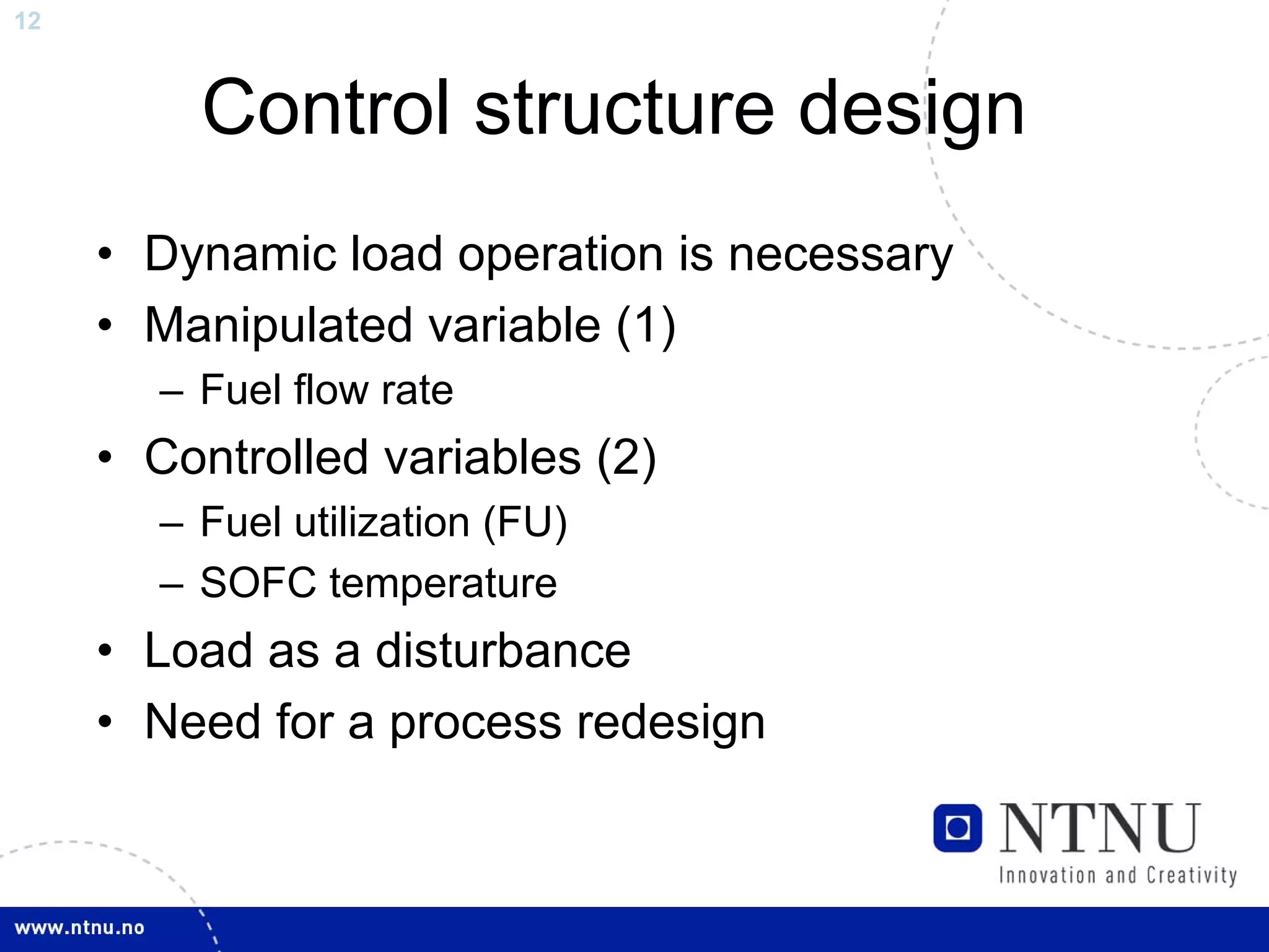
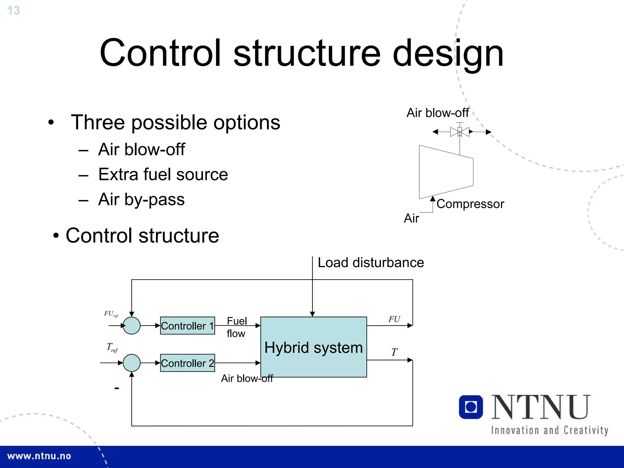
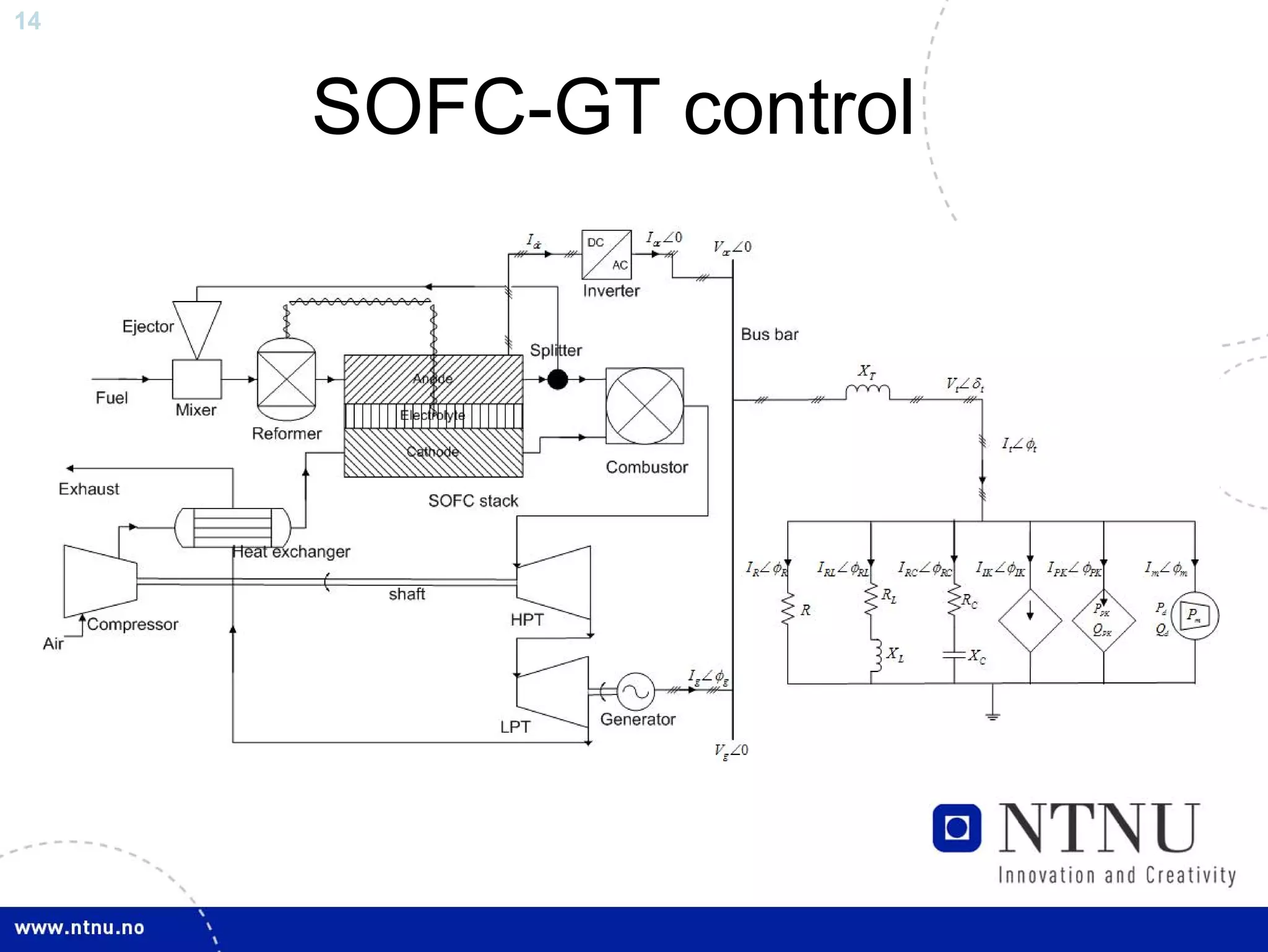
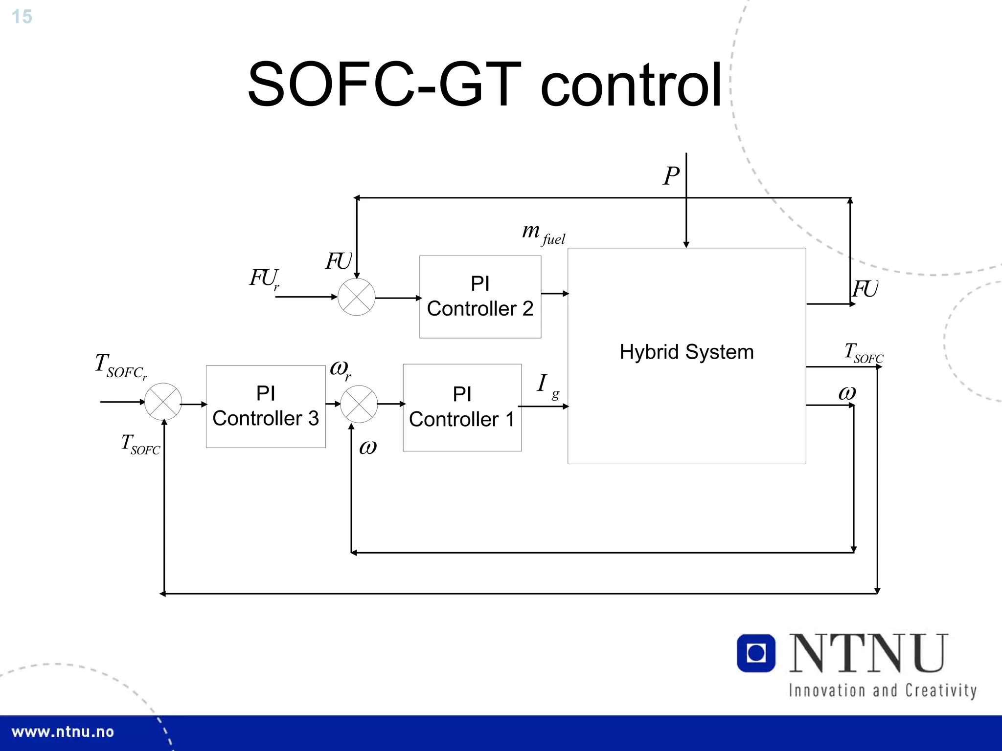
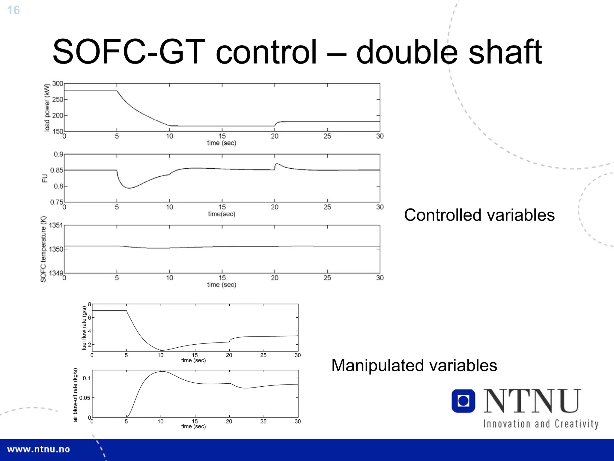
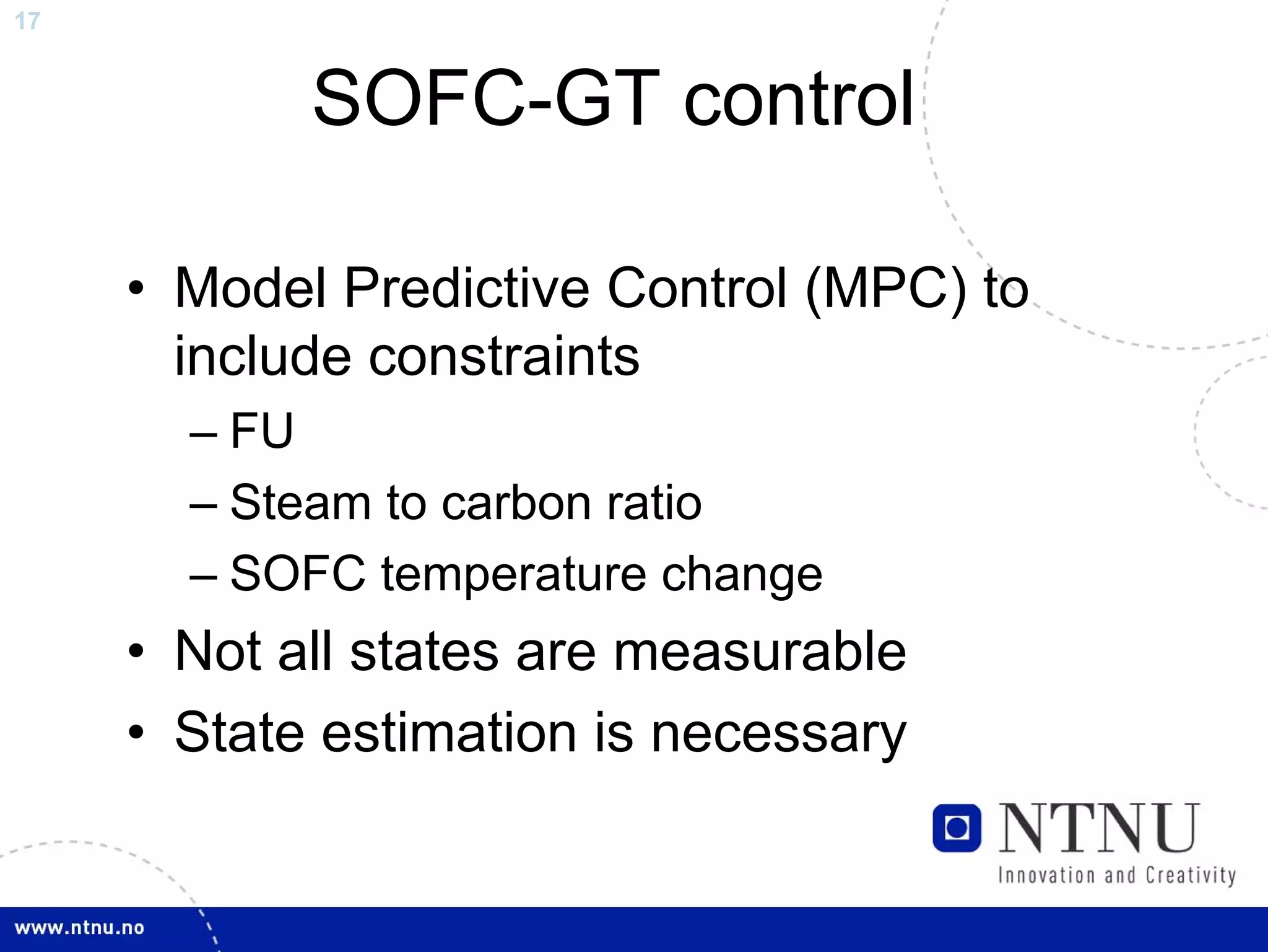
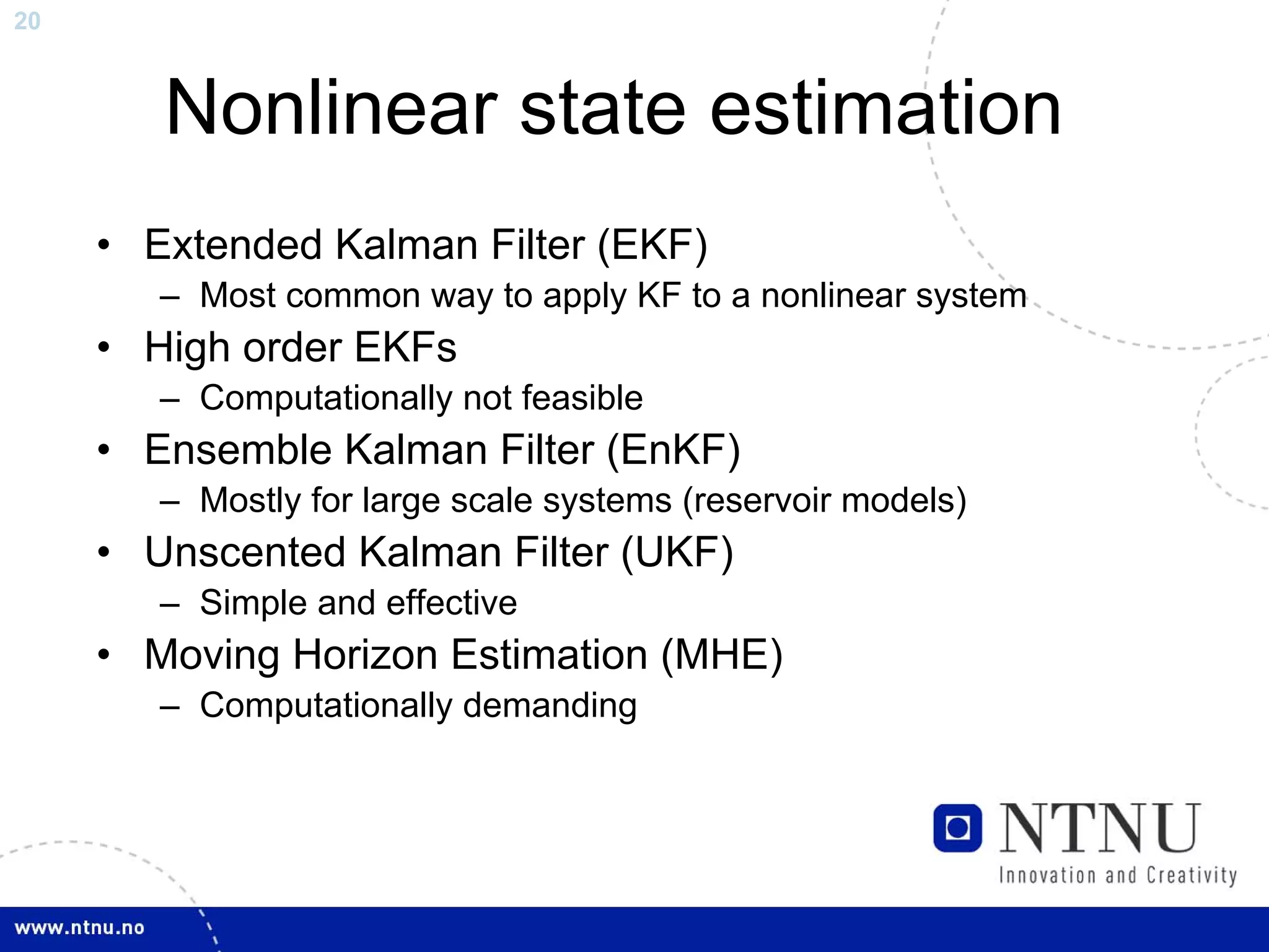
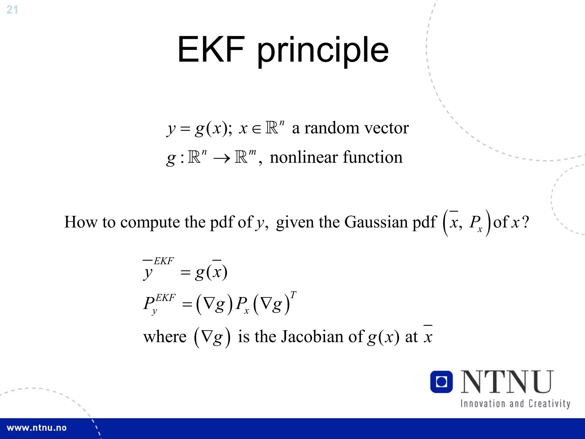
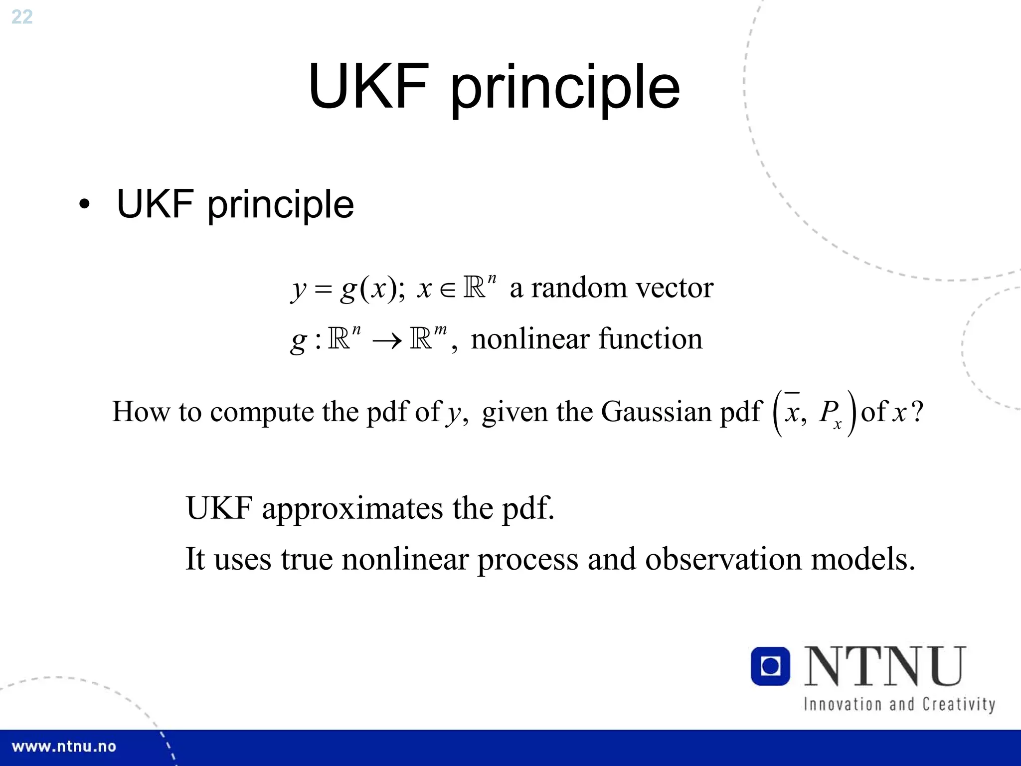

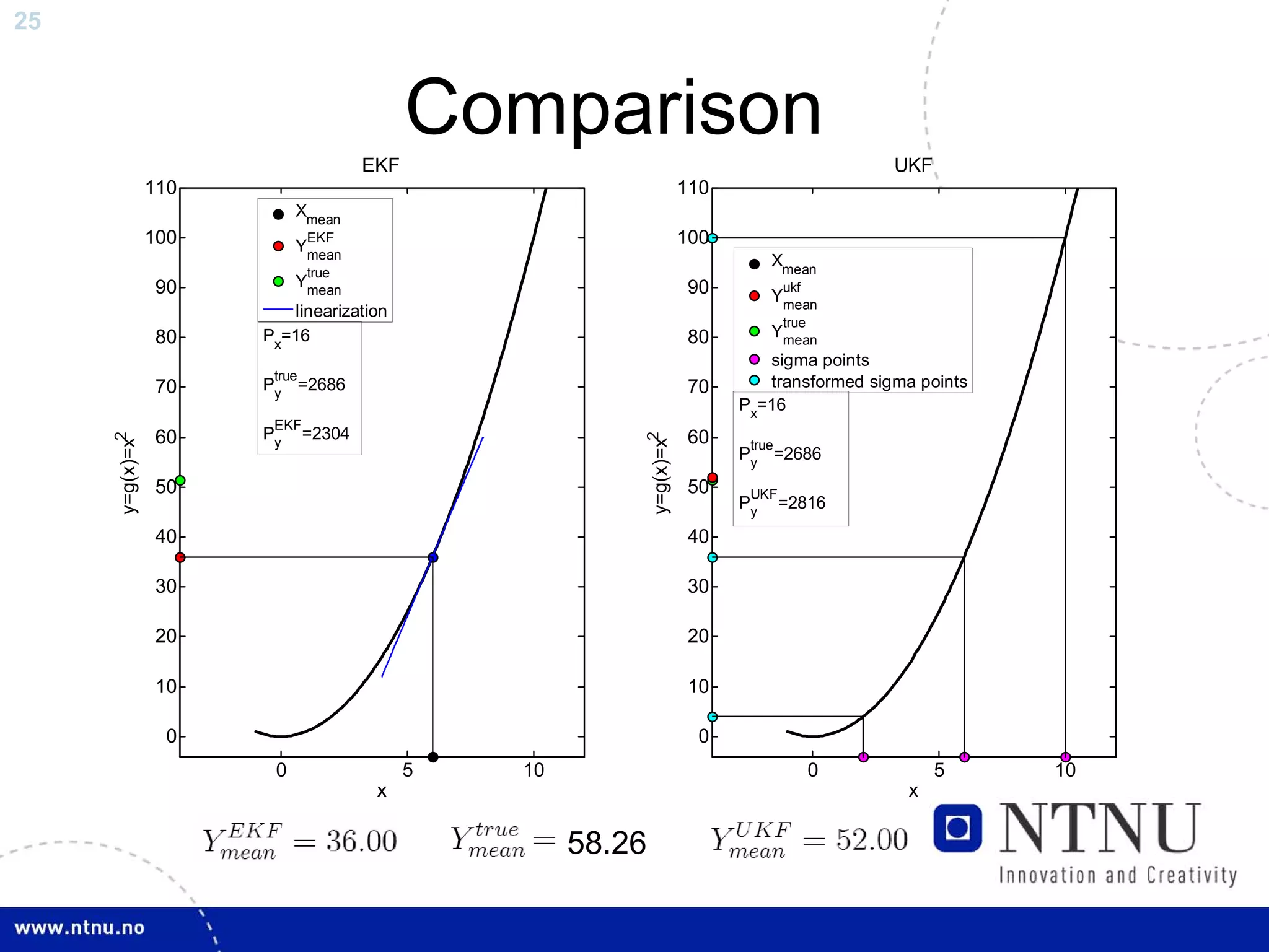
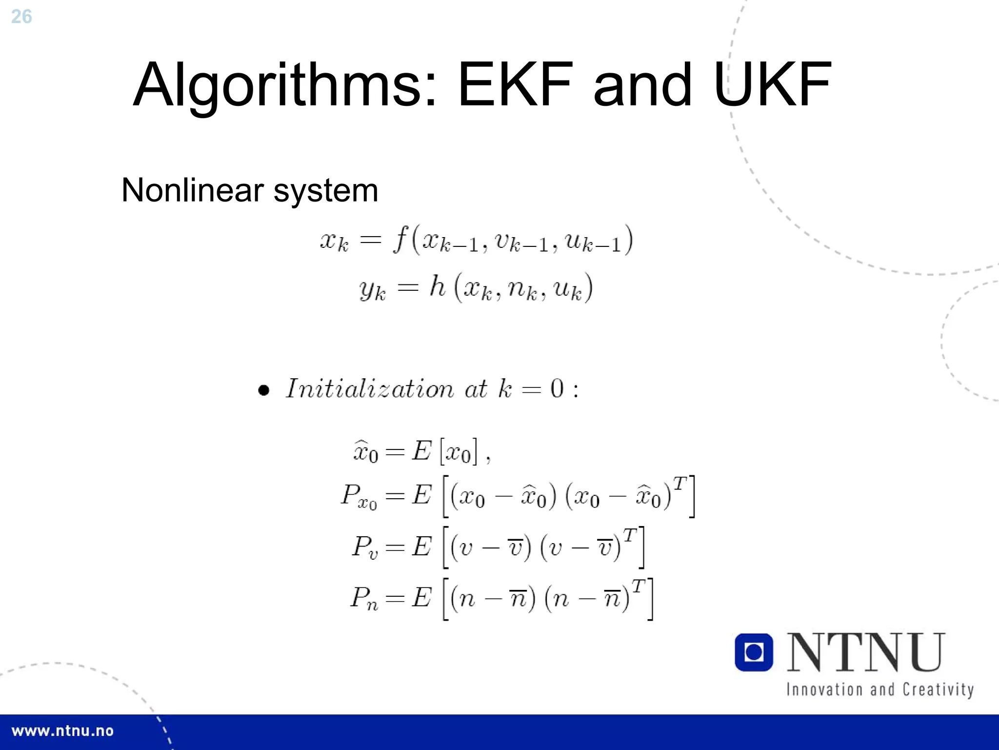
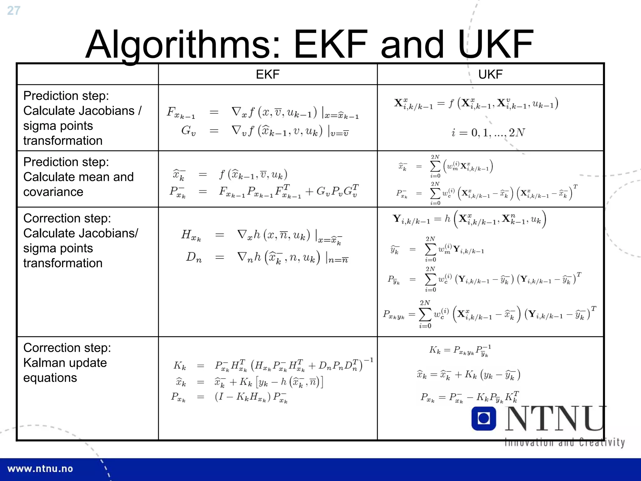
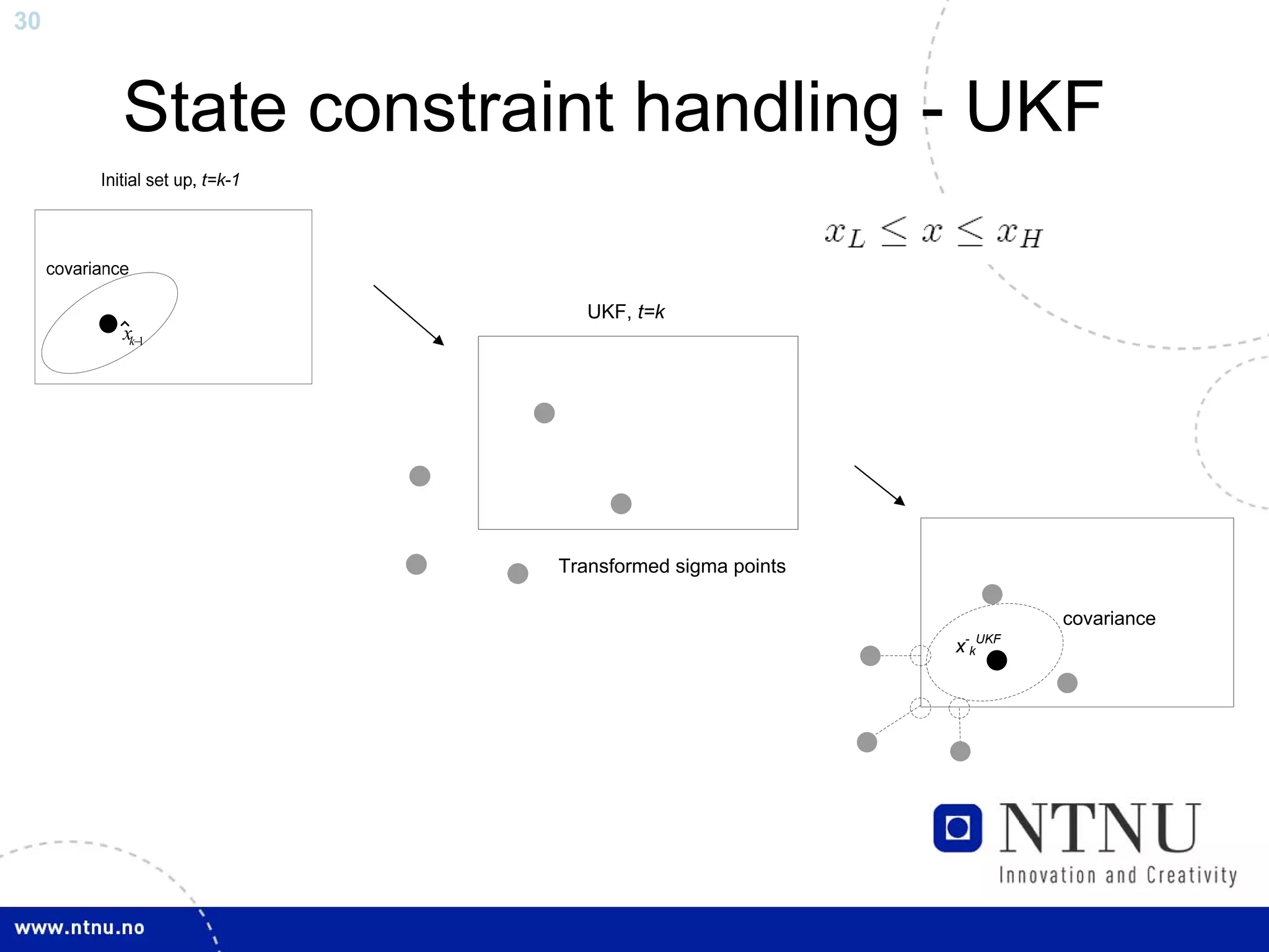
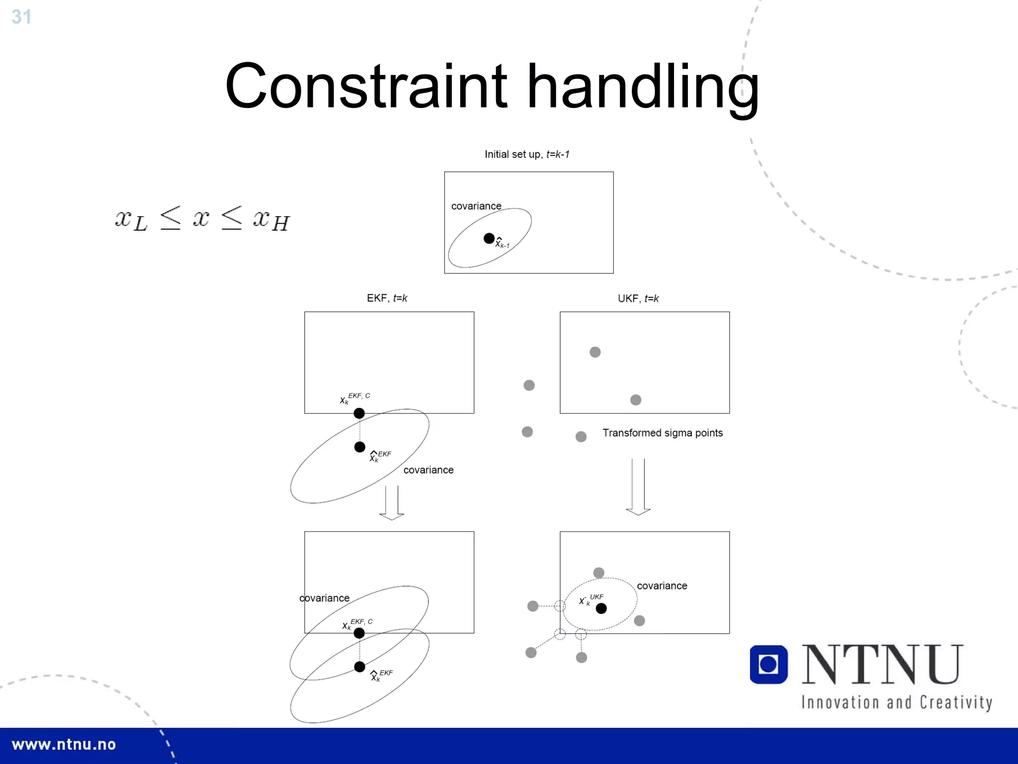
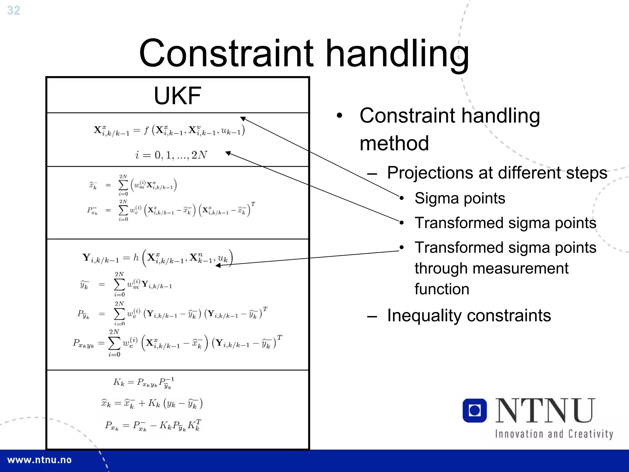
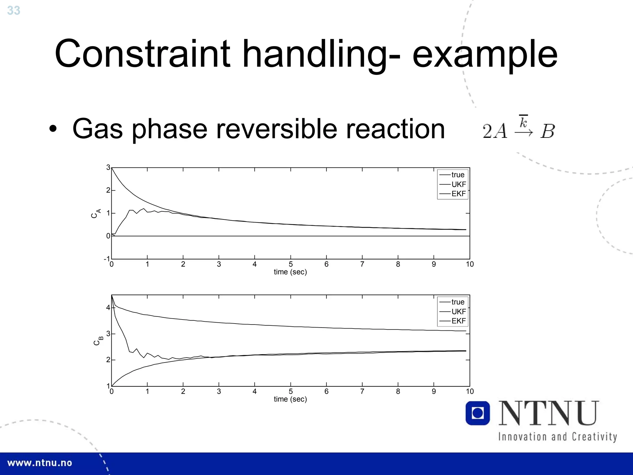
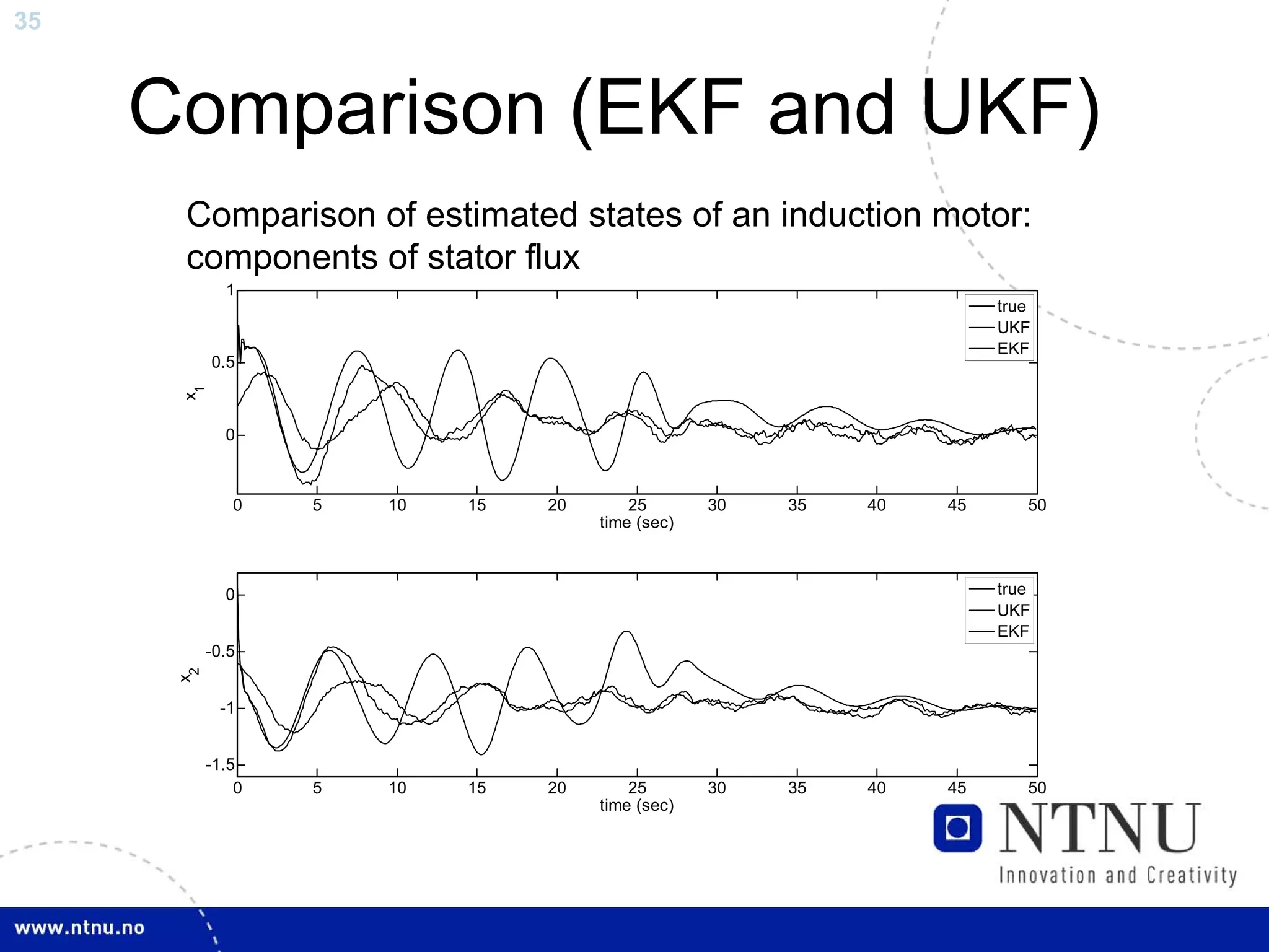
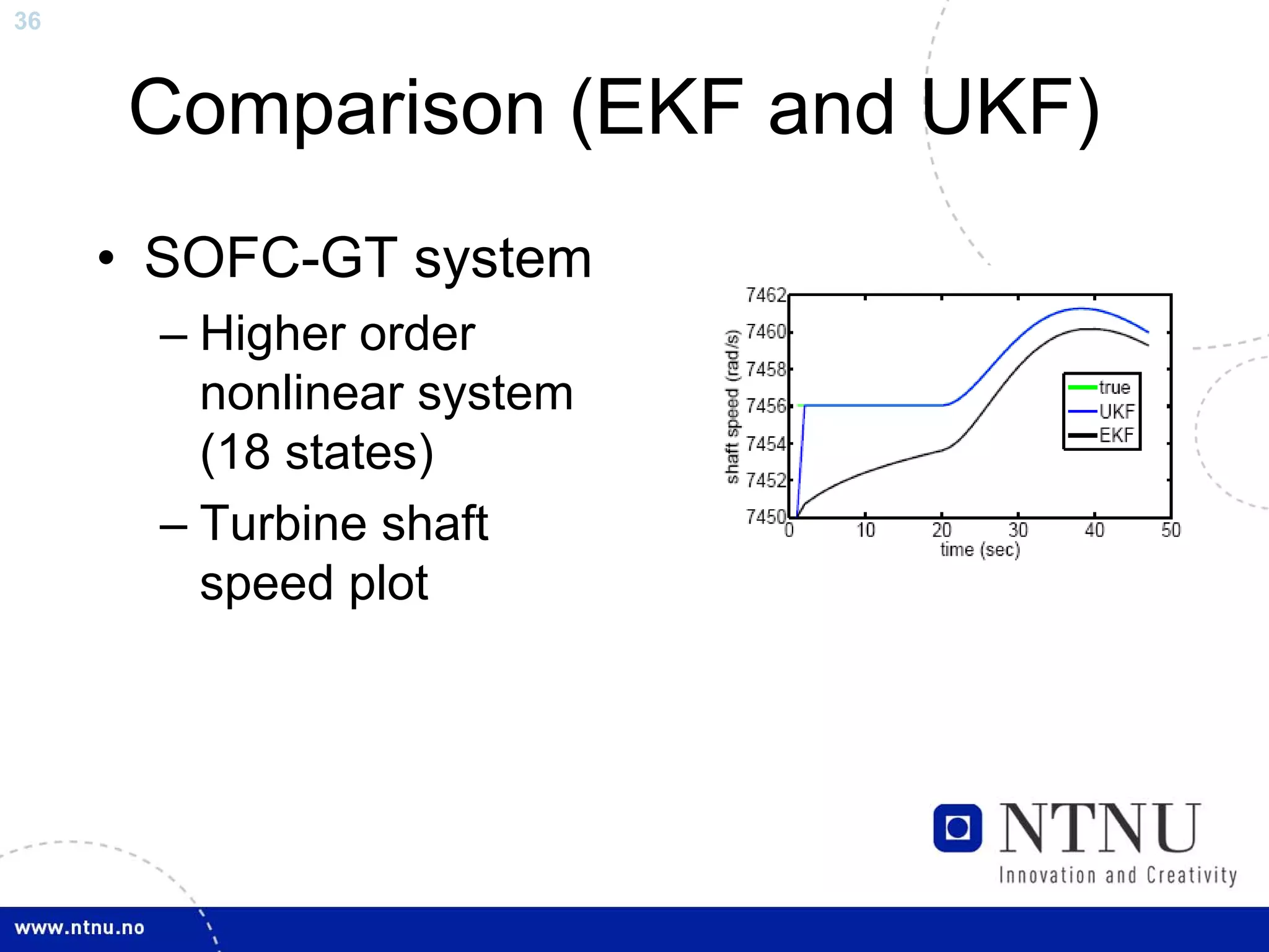


The document discusses control and state estimation techniques applied to solid oxide fuel cell-gas turbine (SOFC-GT) power systems. It motivates modeling and control of SOFC-GT systems to meet increasing energy demands efficiently with low emissions. Nonlinear state estimation using the Extended Kalman Filter (EKF) and Unscented Kalman Filter (UKF) is examined. The UKF is found to provide faster state estimation convergence and better robustness to model errors compared to the EKF for nonlinear systems like the SOFC-GT.


