Downloaded 14 times
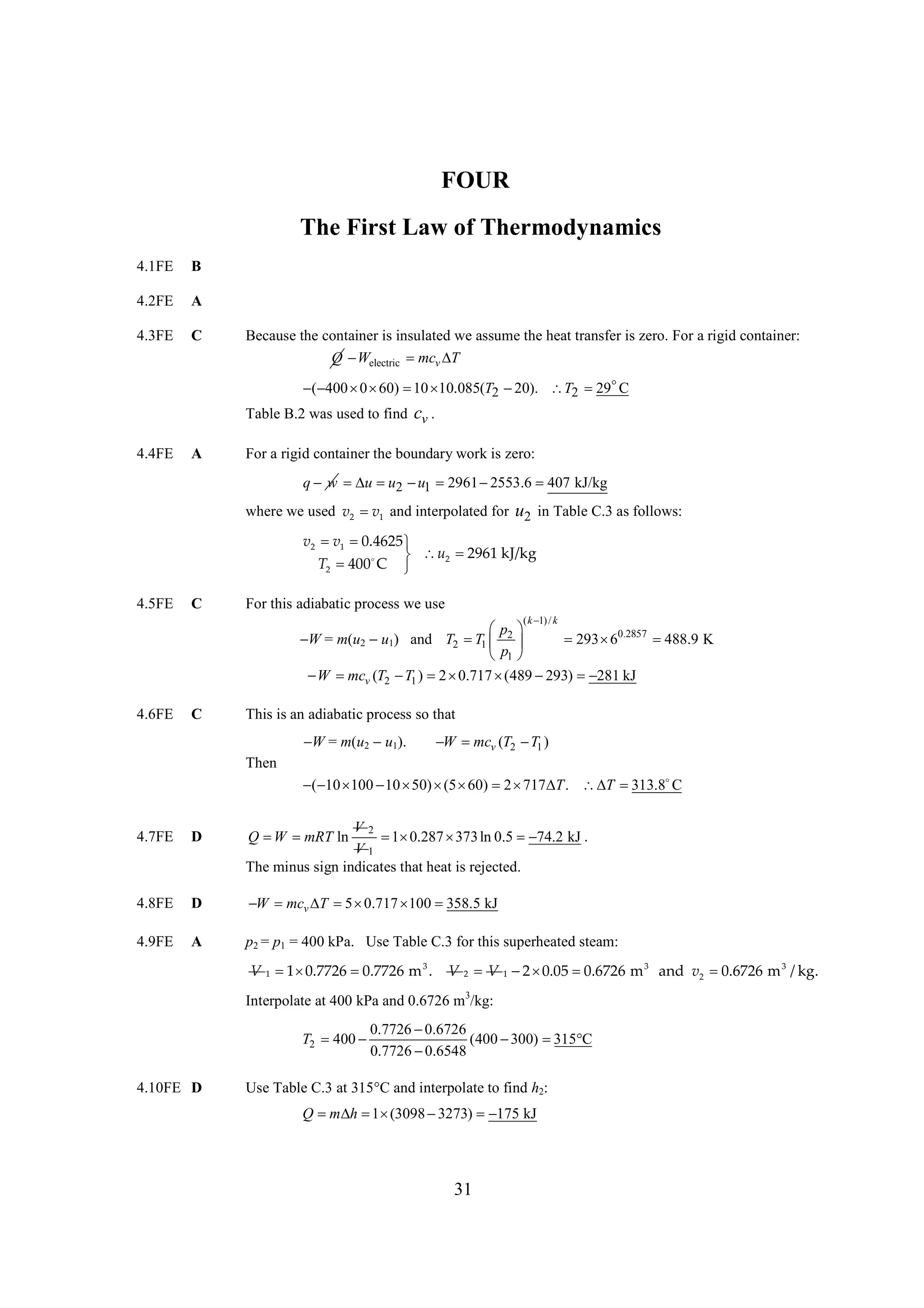
![4.11FE A
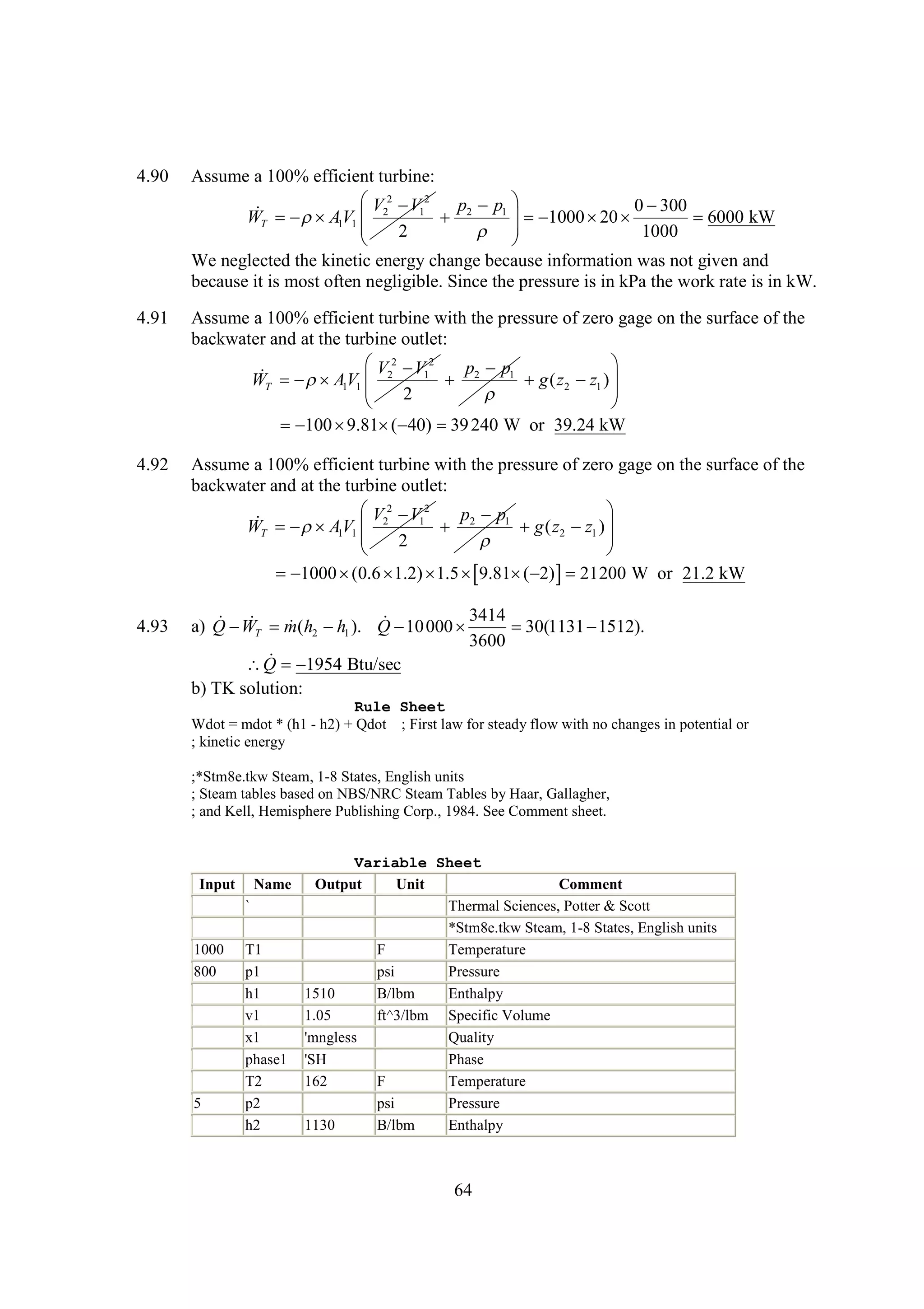
Use Tables C.3 and C.2 with W = 0:
Q (u3 2 )
m
u
1 (1245
2829) = 1584 kJ
We interpolated at 315 in Table C.3 to find u2 = 2829 kJ/kg and used v2 = v3 =
C
0.672 m3/kg which is in the quality region. Then using Table C.2,
x3 = 0.3963 and u3 = 1245 kJ/kg.
4.12FE D
If T = const,
Q
W mRT ln
4.13FE C
p1
100
10 0.287
333 ln
1987 kJ
p2
800
For p = const,
q h2 1
h 3273
604.7
2668 kJ/kg
4.14FE C
For p = const,
Q (h2 1 ).
m
h
170 h2
1 (
3108).
h2
3278 and T2
402 C
We interpolated at 320 in Table C.3 to find h1 and then to find T2.
C
4.15FE D
For p = const,
W ( v2 1 )
mp
v
1 400 (0.7749
0.6784)
38.6 kJ
We interpolated in Table C.3 to find v1 and
v2 and the two temperatures.
4.16FE D
In Table C.3 we observe that u =2949 kJ/kg is between p = 1.6 MPa and 1.8 MPa but
closer to 1.6 MPa so the closest answer is 1.7 MPa.
4.17FE C
Interpolate in Table C.3 and find h = 3459 kJ/kg.
4.18FE C
Use a central difference for accuracy:
3213.6
h
2960.7
cp
2.53 kJ/kg
蚓
T
400
300
4.19FE C
We use q because the mass is not known:
q p (T2 1 )
c
T
2.254
300 676.2 kJ/kg
4.20FE B
The copper gains heat and the water losses an equal amount of heat:
mc c p ,c (T2 w c p , w (30 2 ).
0) m
T
4.21FE B
20
0.38 2
T 10 4.18 2 ). T2
(30 T
25.4
C
First the ice melts and then the ice water heats up:
mi ( i p , w i ) w c p , w w .
h c
T
m
T
10
[333
4.18(T2
0)] 60 4.18 2 ) .
(20 T
4.22FE C
For process 1:
Q = W =100 = a.
For process 2:
b = 40 + 60 = 100.
W or 100 .
100 40 100 60 c
Q
32
c
80
T2 = 5.85蚓](https://image.slidesharecdn.com/ch04-131023024337-phpapp02/75/thermal-science-Ch-04-2-2048.jpg)
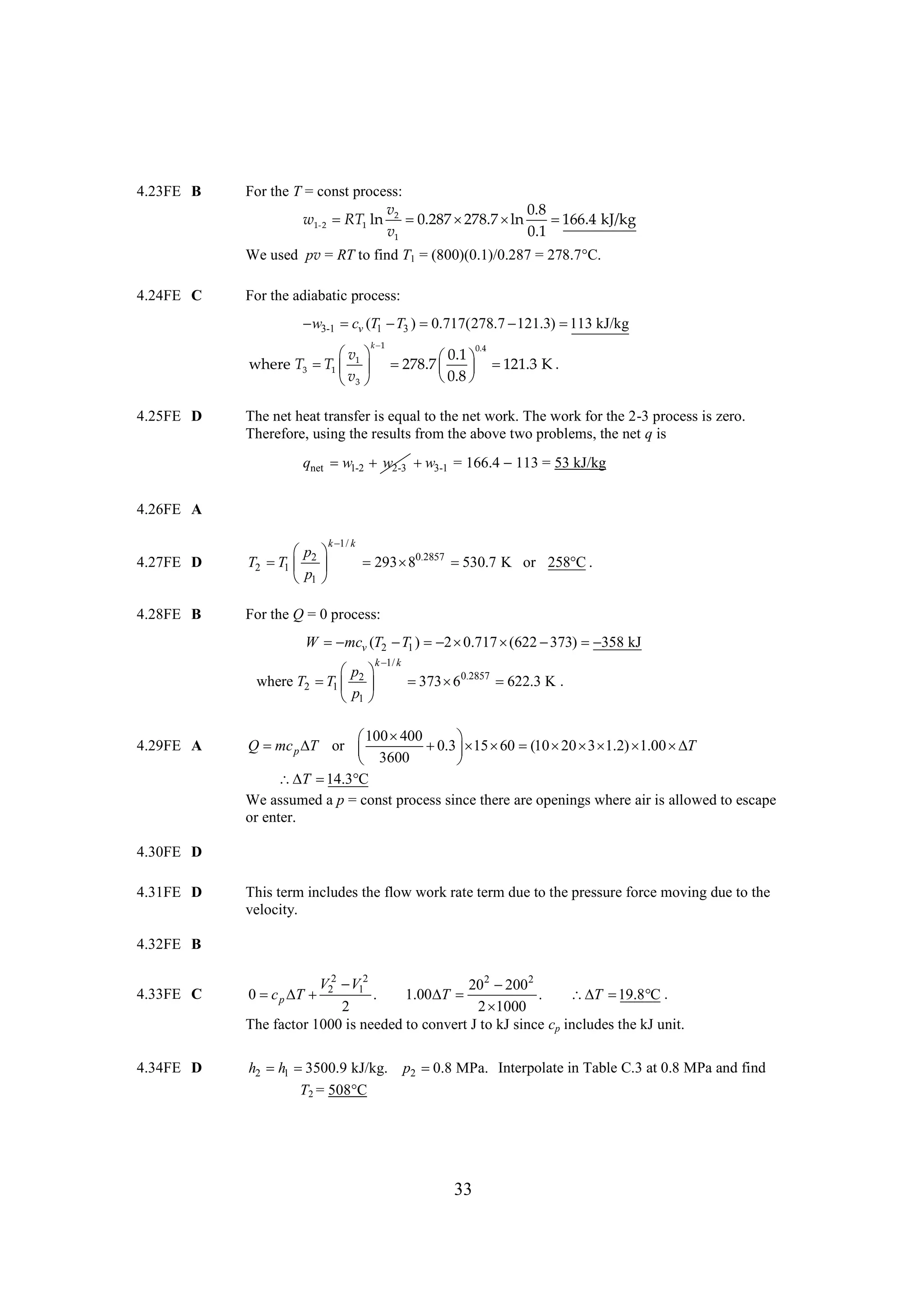
![4.1
Qnet net
W
100 m
9.81 m
3.
3.398 kg
4.2
1
1
Qnet net . Qnet mV 2
W
1500 2
30
675000 J
2
2
4.3
0.
F
pA patm A
mg
0
p 2
0.05 10 9.81 000 2. p 490 Pa
100
0.05
112
Q .
W
U
U 300 (112 490 2 )
0.05
0.2 123.3 J
4.4
24)] ft-lbf or
U Q W
2 778 [ 600 (2 1/
381
0.49 Btu
4.5
a) 20 kJ E2 E2 kJ
E Q W
5 15
7.
22
b) Q 6 kJ. E2 E2 kJ
E W
3 3
8 6.
14
c) W E 40 25 kJ. kJ
Q
(30 15)
E 30 15 15
d) W E kJ. 20 1 . E1 kJ
Q
10 20
30
10 E
10
e) Q kJ. kJ
E W
8 6 10
4
E
8 6
14
4.6
a 1-2 1-2 U kJ
W
Q
200 0
200
( )cycle 0. 0
U
c 400 1200 c
0.
800 kJ
b 2-3 2-3 U kJ
W
Q
800 800 0
d 3-4 3-4 400
Q
U W
600 1000 kJ
e 4-1 4-1 U
W
Q
0 ( 1200)
1200 kJ or we could use Qnet net
W
4.7
a 1-2 1-2 200 kJ
Q
E W
100 100
( )cycle 100
E
0.
c 200 c kJ
0.
100
b 2-3 2-3 kJ
Q
E W
100 50 50
d 3-1 3-1 E
W
Q
100 ( 200)
300 kJ or we could use Qnet net
W
35](https://image.slidesharecdn.com/ch04-131023024337-phpapp02/75/thermal-science-Ch-04-5-2048.jpg)
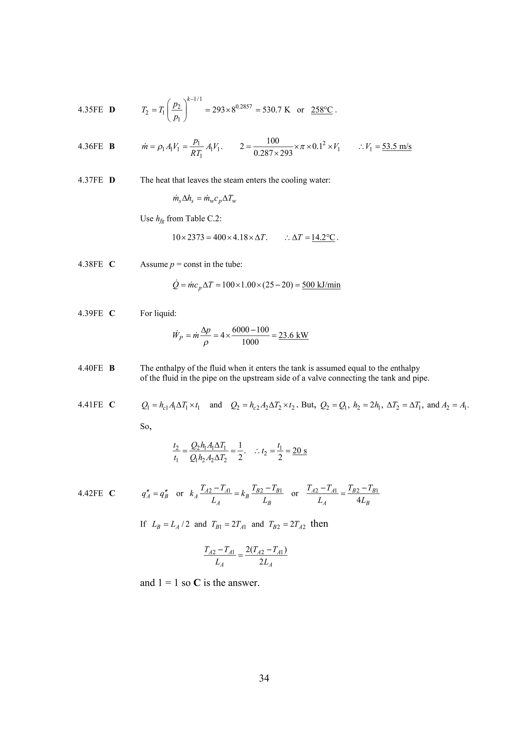
![4.8
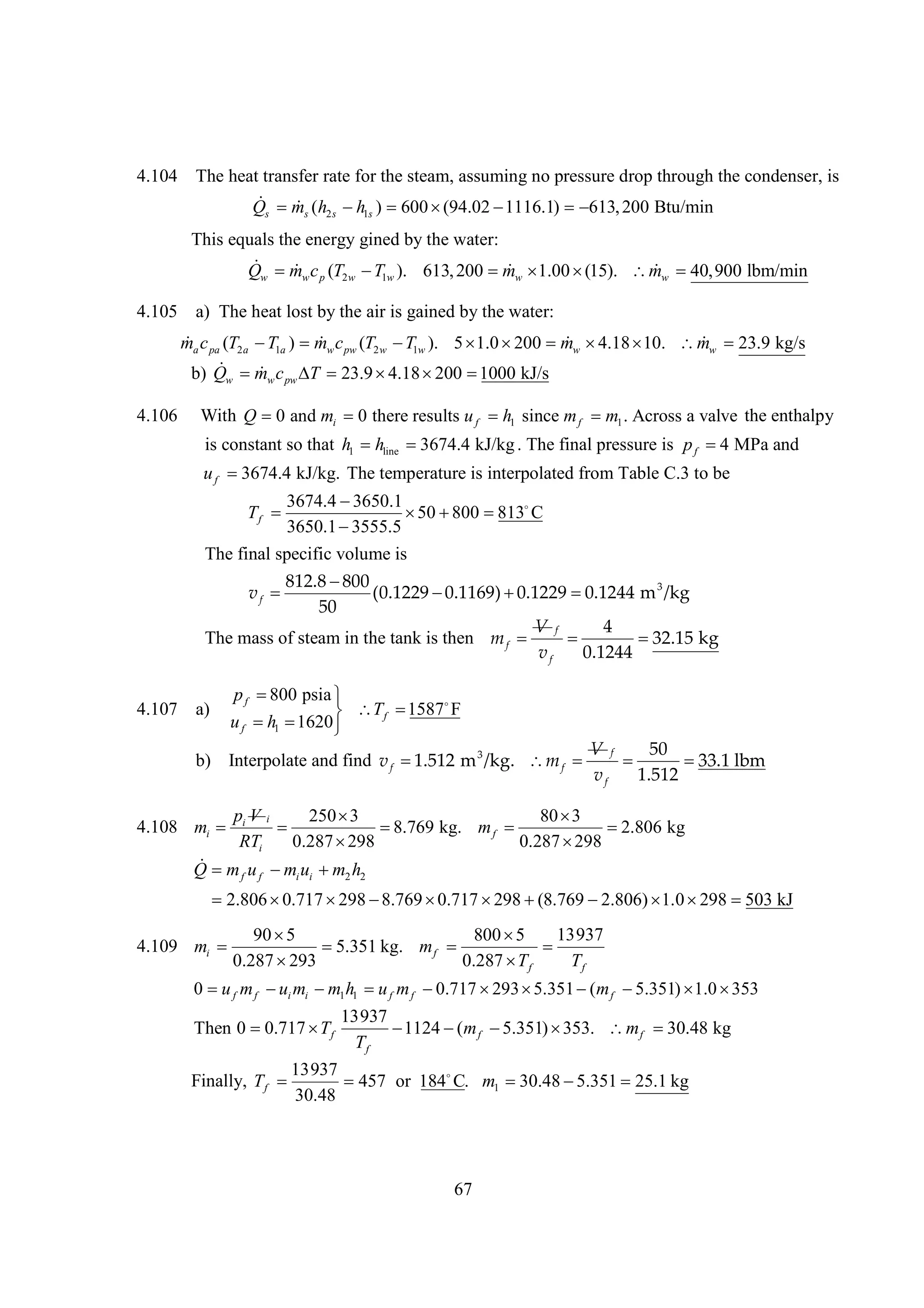
First, find the initial pressure in the cylinder:
W
60
9.81
p patm
000 000 Pa
100
119
A
2
0.1
Now, apply the 1st law adding the work of the pressure force and the work to
compress the spring:
1
Q .
W
U
Q pA Kx 2 )
(
h
U
2
1
200
U
(119 000 2
0.1 0.05 000 2 ) J
50
0.05
49
2
4.9
W1-2 6 000 J.
VI t
5 (20 60) 36
Q1-2 1-2 2-1 W2-1 )cycle 0. Q2-1 1-2 kJ
W
Q
( U
W
36
4.10
Q 000 600 J or 377.6 kJ
U W
400
12 3 (6 60 60) 377
4.11
Q U 300 000 84 000 J or kJ
W
12 10 (30 60)
84
4.12
Q
U W 8000 /1055
110 15 (2 60 60)
3260 Btu
w e t f t 15 cne s tBus
hr h a o 05 ovr Jo t .
e e cr
t
’
4.13
The only transfer of energy across the boundary of the system is via the
electrical wires leading to the refrigerator. The 1st law is
Q . ) 2
W
U
U
W
( VI t
0.746 2686 kJ
(30 60)
V
0.3
(u2 1 )
u
(3655.3
2621.9)
1505 kJ
v
0.206
4.14
Q W
m u
4.15
a) Q W
m u
V
(u2 1 )
u
v
0.2
1000
{u2
[669.9
0.8(2567.4
669.9)]}
0.0011
0.8(.3157
.0011)
u2
3452 kJ/kg and v2
0.2528 m 3 /kg . We must find where in Table C.3
this state exists. After checking the table we interpolate for the following:
p2 MPa, v2
1.5
0.2528, u2
3216 : T2
556 C
686
C
T2
p2 MPa, v2
2.0
0.2528, u2
3706 : T2
826 C
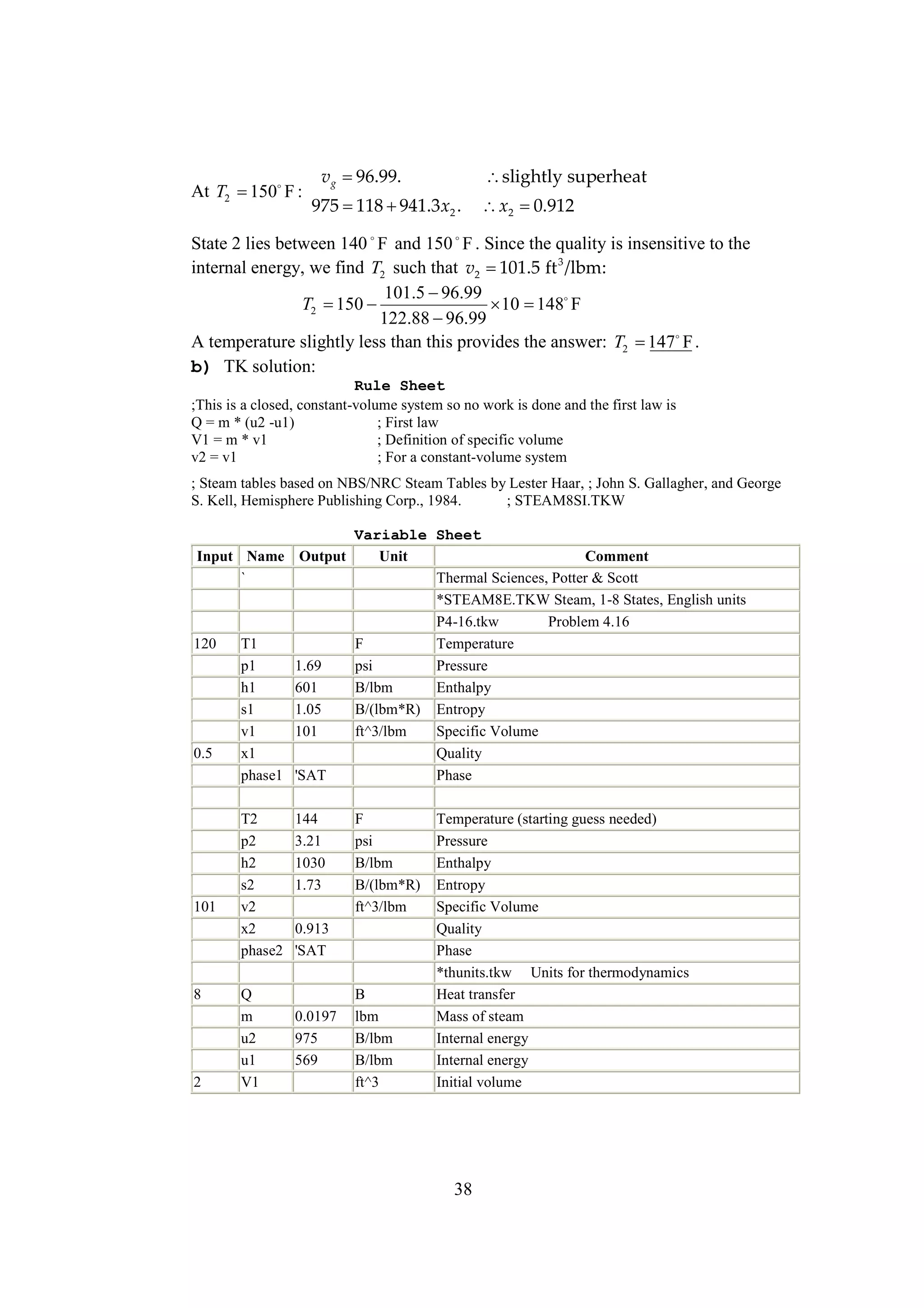
b) TK solution:
Rule Sheet
;This is a closed, constant-volume system so no work is done and the first law is
Q = m * (u2 -u1)
; First law
V1 = m * v1
; Definition of specific volume
v2 = v1 ; For a constant-volume system
; Steam tables based on NBS/NRC Steam Tables by Lester Haar, ; John S. Gallagher, and George S.
Kell, Hemisphere Publishing Corp., 1984.
; STEAM8SI.TKW
36](https://image.slidesharecdn.com/ch04-131023024337-phpapp02/75/thermal-science-Ch-04-6-2048.jpg)
![V 100 / 1728
0.01633 lbm
v
3.544
120
144
100
Q m(u2 1 )
u
W 0.01633{1371.5
[312.3
0.95(796)]}
(7.208
)
778
1728
6.28 Btu
4.17 v1
0.0179
0.95(3.73
0.0179)
3.544. m
4.18
First, find the mass: m
V 1 0.004
0.0302 kg . The 1st law is Q m(u2 1 )
W
u
v1
0.1325
which takes the form
40
1500
0.03019( v2
0.1325)
0.0302(u2
2598) or 124.4 v2
45.3
0.0302u2
The above equation has two variables but the steam tables represent the 2nd equation.
'
This requires trial-and-error (let u2 be the u2 from the above equation):
'
At T2
600, p2 : v2
1.5
.2668, u2
3294. u2
3720
'
At T2
780, p2 : v2
1.5
.3230, u2
3622. u2
3636 T2
785 C
'
At T2
800, p2 : v2
1.5
.3292, u2
3627. u2
3720
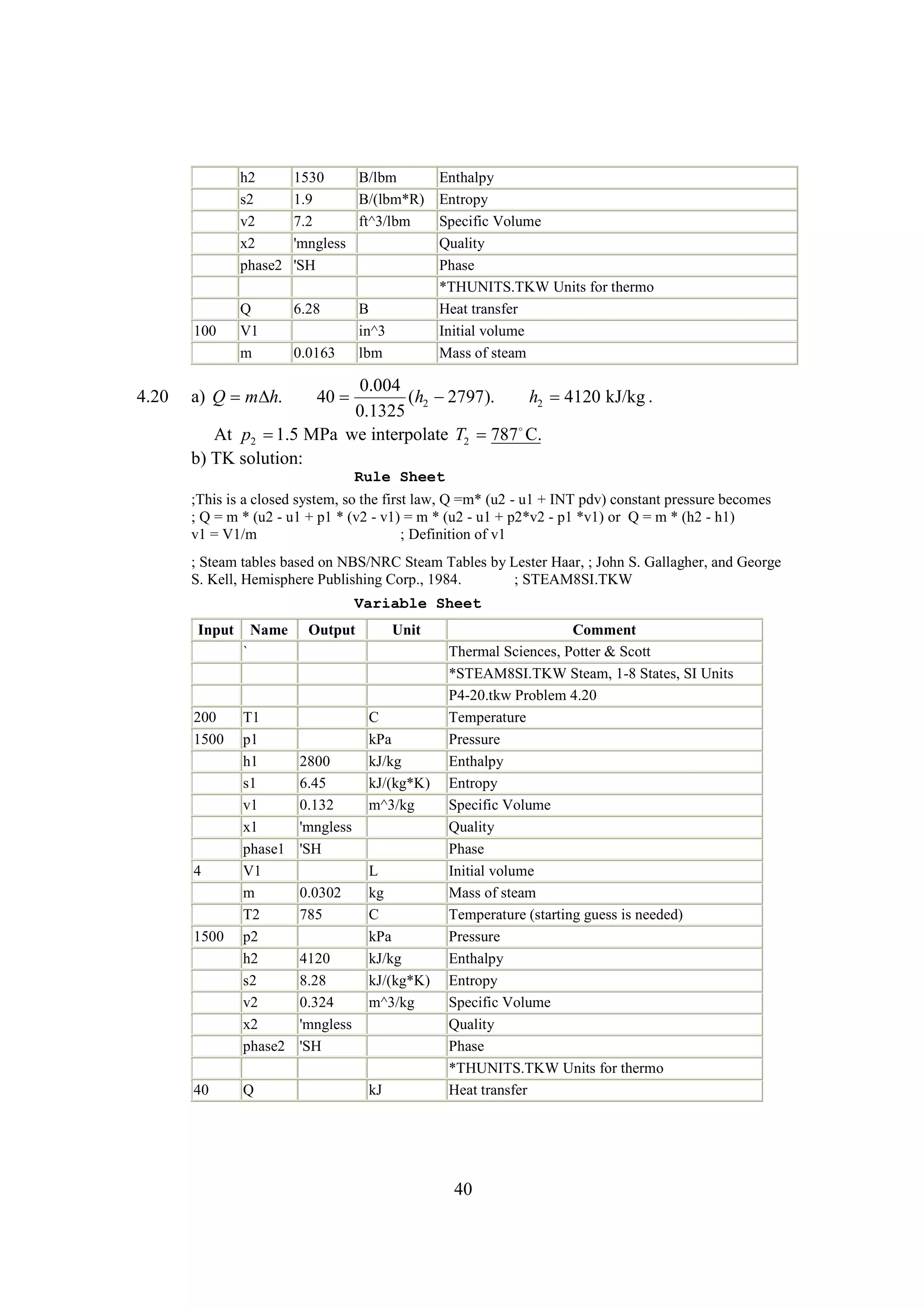
4.19
100 /1728
a) Q m(h2 1 )
h
{1531.5
[312.7
0.95(878.5)]}
6.27 Btu
3.544
b) TK solution:
Rule Sheet
;This is a closed system, so the first law, Q =m* (u2 - u1 + INT pdv), at constant pressure
becomes
; Q = m * (u2 - u1 + p1 * (v2 - v1) = m * (u2 - u1 + p2*v2 - p1 *v1) or
Q = m * (h2 - h1)
v1 = V1/m
; Definition of v1
; Steam tables based on NBS/NRC Steam Tables by Lester Haar, ; John S. Gallagher, ;and George
S. Kell, Hemisphere Publishing Corp., 1984. ; STEAM8E.TKW
Variable Sheet
Input Name
`
120
0.95
1000
120
T1
p1
h1
s1
v1
x1
phase1
T2
p2
Output
341
1150
1.53
3.54
'SAT
Unit
Comment
Thermal Sciences, Potter & Scott
*STEAM8E.TKW Steam, 1-8 States, English units
P4-19.tkw Problem 4.19
F
Temperature
psi
Pressure
B/lbm
Enthalpy
B/(lbm*R) Entropy
ft^3/lbm
Specific Volume
Quality
Phase
F
Temperature
psi
Pressure
39](https://image.slidesharecdn.com/ch04-131023024337-phpapp02/75/thermal-science-Ch-04-9-2048.jpg)
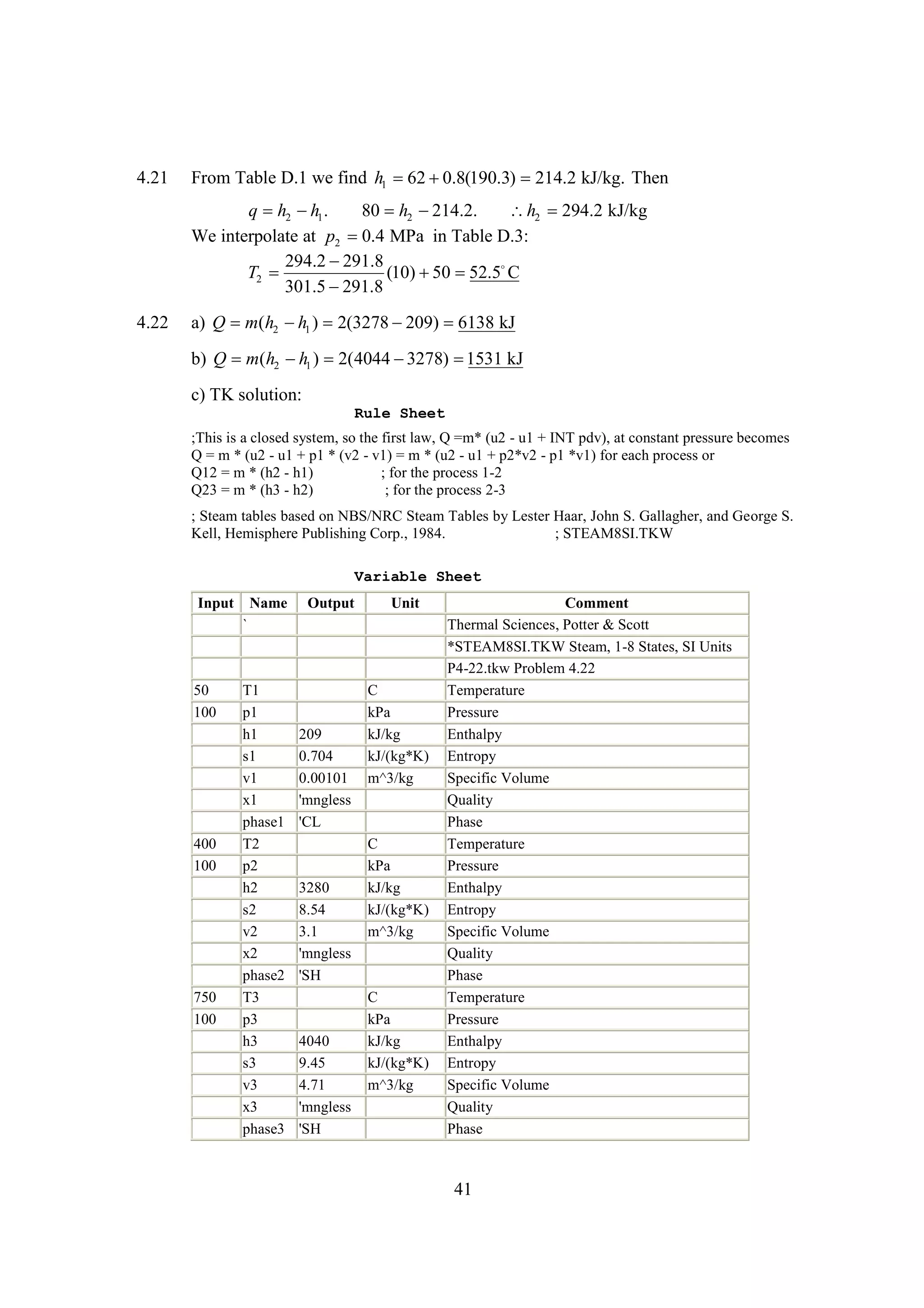
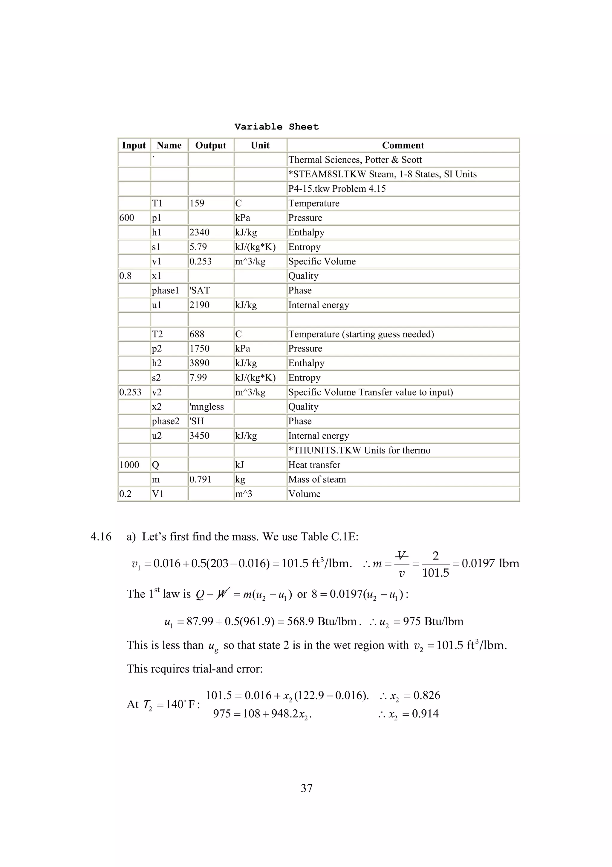
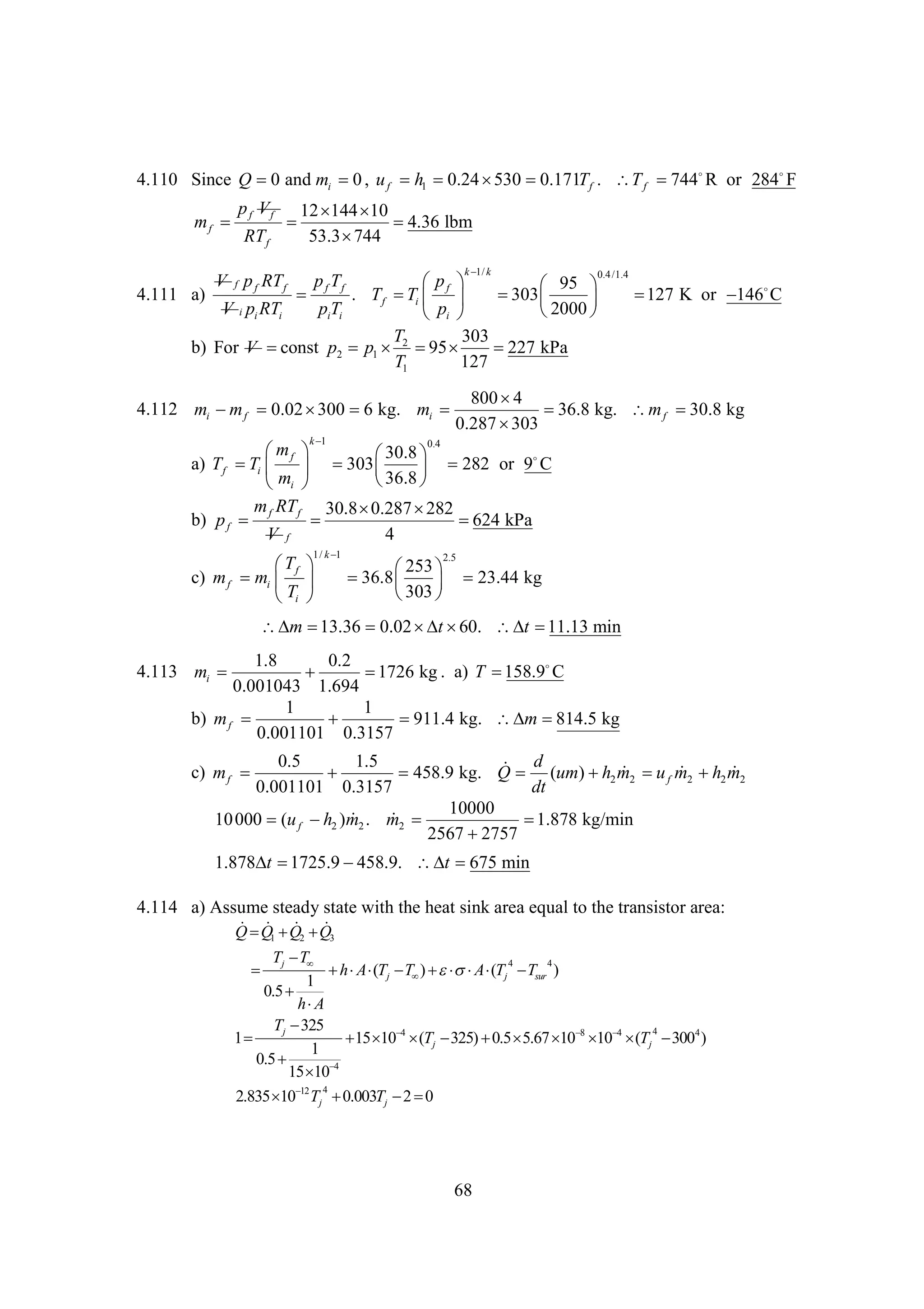
![d) The error in (a) is
2.6% and that in (b) is 1.1% assuming that of (c) is the
best answer. All three methods are acceptable for the temperature range of
this problem.
4.29
a) mc p (T2 1 ) 2
H
T
.006
(600
400) 402 kJ
.213
10 3
.031
10 6
b) 2
H
.946 200
(6002 2 )
400
(6003 3 ) 418 kJ
400
2
3
c) m(h2 1 ) 2(607
H
h
401) 412 kJ
4.30
water mc p 2
H
T
4.18(60 418 kJ
10)
ice mc p 2
H
T
1.86[ kJ
10 ( 60)] 186
where we averaged the (c p )ice between and in Table B.4.
10 C
60 C
4.31
Assume that all of the ice melts. The ice warms up to 0 , melts at 0 , then
C
C
warms up to the final temperature T2 . Fr, t f dh m so t ice:
it e si t as fh
s l’ n e
e
6
V 16
8 10
mi
0.1174 kg
v
0.00109
where we found v in Table C.5. Energy is conserved so that the heat gained by the
ice equals the heat lost by the water:
mi p )i ( )i if c p ) w ( )iw mw (c p ) w ( ) w
(c
T
h (
T
T
0.1174
2.1 10 330 4.18(T2 (1000 )
0)
10 3 4.18(20 2 )
T
T2
9.07
C
4.32
a) Assume the ice melts and then the water is heated:
Q m(c p )i ( )i if (c p ) w ( ) w
T
mh m
T
2000 2.3 T2 T2
1.89 60 330 4.18 .
102 C
b) Assume the ice melts and then the water is heated:
Q mhif (c p ) w ( ) w
m
T
2000 2.3 T2 T2
330 4.18 .
129.1
C
This is in the superheat region so the above temperature is too high. The water
must first vaporize at T2
as e n m a r
120.2 ,o ht t f at pr ue
C s t ’ h i le e t .
46](https://image.slidesharecdn.com/ch04-131023024337-phpapp02/75/thermal-science-Ch-04-16-2048.jpg)
![1
10
30
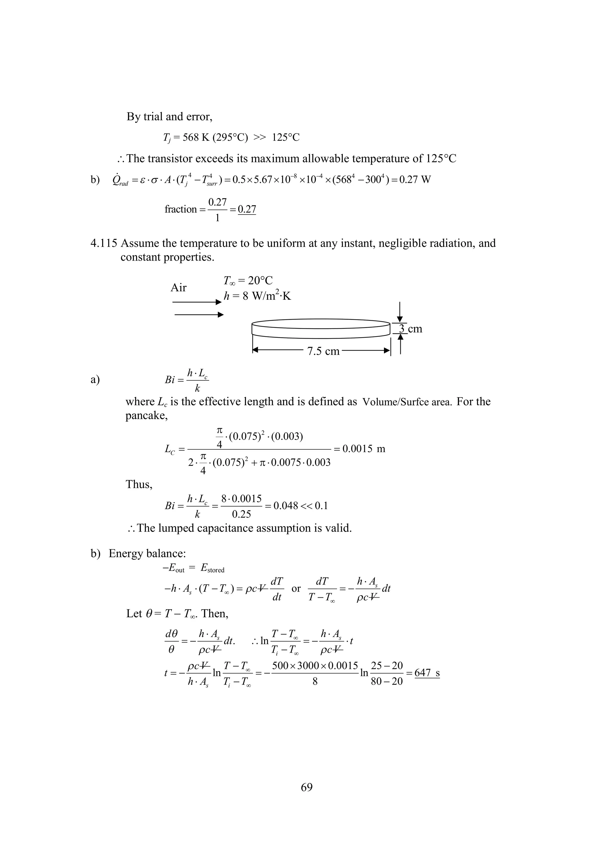
4.94
4.95
v2
x2
phase2
Wdot
mdot
Qdot
73.5
ft^3/lbm
'SAT
MW
lbm/s
B/s
-1950
Specific Volume
Quality
Phase
*THUNITS.TKW Units for thermo
Power output
Mass flow rate
Heat is removed at a rate of 1950 B/s
1000
m(
WT h2 1 )
h
(1116.1
1623.8)
8462 Btu/sec or 11,970 hp
60
m
1000 / 60
V
230 fps
A 2 /173.75
2
where we used v.
1/
h1
3445.2 kJ/kg, h2 h f x2 h fg 251.4
0.9(2358.3) 2374 kJ/kg
m(
WT h2 1 )
h
6(2374
3445)
6430 kW
m
6
V2
82.2 m/s
2
A
0.4 /[0.001
0.9(7.649
0.001)]
4.96
4.97
600
2
0.05 100
0.287
373
A2V2 AV1 . V2
18.17 m/s
2
1 1
140
2
0.2
0.287
253
600
1 1
m AV1
2 4.402 kg/s
0.05 100
0.287
373
V 2 12
V
18.17 2 2
100
m
WT c p (T2 1 ) 2
T
4.402
1.00( 20 100)
539 kW
2
2
1000
T eat “00 it dnm nt o t k ec nrye cne s t k
h f o 10”n h eo i o fh i t ee t m ovr W o W.
cr
e
ar e ni
g r
t
800
1 1
m AV1
2
0.05 20 0.9257 kg/s
0.287
473
Q mc (T ) 0.9257
T W
1.0(200
20) ( 400) kJ/s
233
p
2
1
S
The negative sign indicates a heat loss, as expected.
4.98
450
Q mc p (T2 1 )
T WS
2
.06 150 1.0 (20 100)
500
70.5 kJ/s
.287
373
65](https://image.slidesharecdn.com/ch04-131023024337-phpapp02/75/thermal-science-Ch-04-35-2048.jpg)
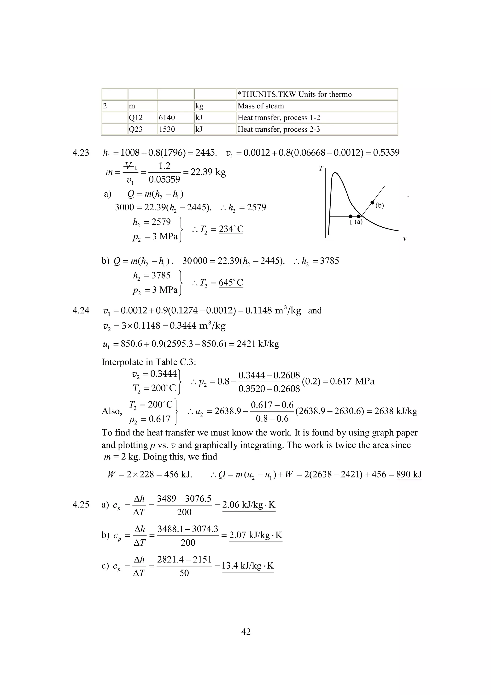
![4.99
Fr, t cl leh vl ie:
it e s a u tt e ci
s l’ c a e o ts
m
30
30
V1
5.509 fps, V2
137.7 fps
2
A1 62.4 /144
2
62.4 2 /144
0.4
1
2 V2
V 1 p2 p1
Q WS m 2
2
137.7 2
5.5092 (14.7 1 )
P 144
0
30
.
142
p1 psia
32.2
62.4
2
The factor 32.2 above converts slugs to lbm.
4.100 The energy equation: V22 12 c p (T1 2 ) 202
V
2
T
2 1.0(293 2 )
T
p1
AV1 A2V2
1
2
RT1
80
2
4
V2
20 5.384 kg/m 2
s
2
0.287
293 2
3
Assume an adiabatic expansion using v :
1/
Continuity equation: AV1 A2V2 .
1 1
2
k-1
T2 2
T2
293
298.9
or 0.4
T1 1
[80 / 0.287 0.4
293]
2
The above three equations include three unknowns , V2 , and T2 . They are solved
2
by trial-and-error to give
3.47 kg/m3 , V2
1.55 m/s and T2 219
C
2
k /k
1
p
4.101 a) Assume an adiabatic process: T2 1 2
T
p
1
0.4 /1.4
585
468
85
812 K or 539
C
2 12
2 2
V V
V 100
b) 0 2
p (T2 1 ) 2
c
T
1.0(812
468) V2
.
835 m/s
1000
2
2
p
p
585 2
0.1 100 812
c) 2 ( d 22 / 4)V2 1 12 1 . d22
r V
. d2
0.239 m
RT2
RT1
185 / 4
468 835
p
80
4.102 a) m AV
2
0.05 200 1.672 kg/s
RT
0.297
253
V22 12
V
152 2
200
b) 0
p (T2 1 ). 0
c
T
1.042(T2
20). T2
0.91 C
2
2
1000
V 2 12
V
502 2
600
4.103 0 2
2 1. 0
h h
2
h 1154.
2
2
1000
P2 20 psia
T2 238 F
h2
1161
66
h2
1161 Btu/lbm](https://image.slidesharecdn.com/ch04-131023024337-phpapp02/75/thermal-science-Ch-04-36-2048.jpg)

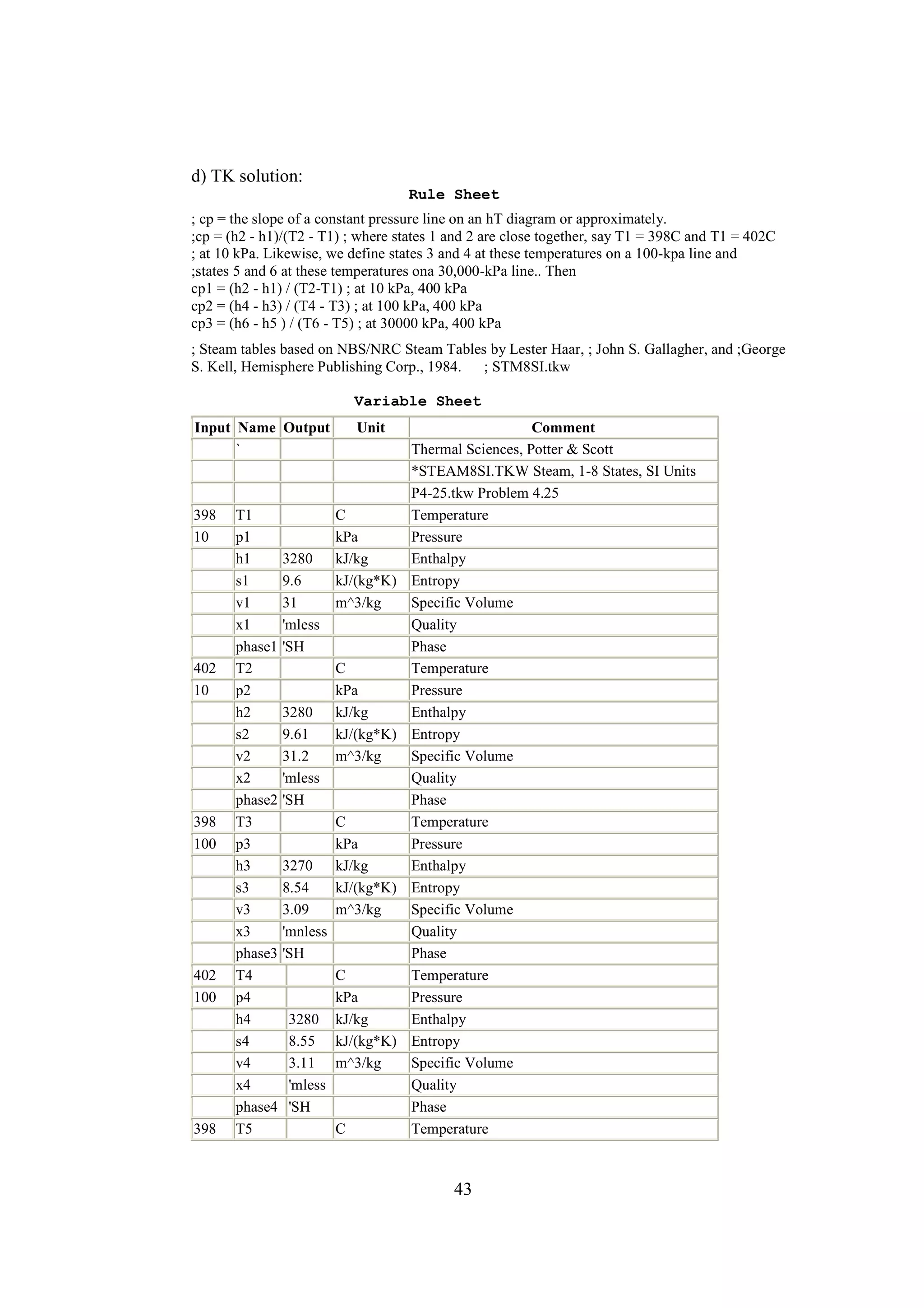
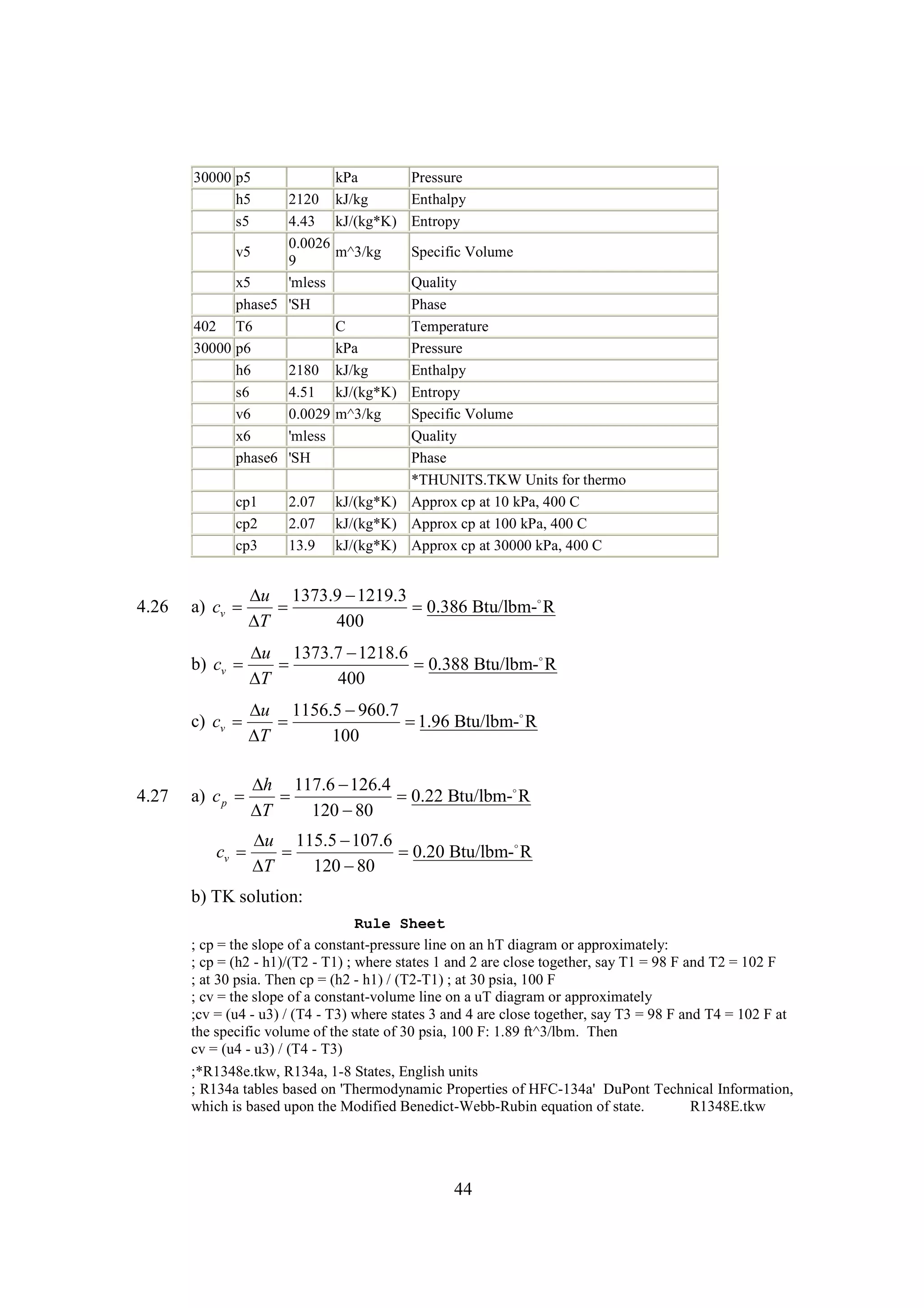
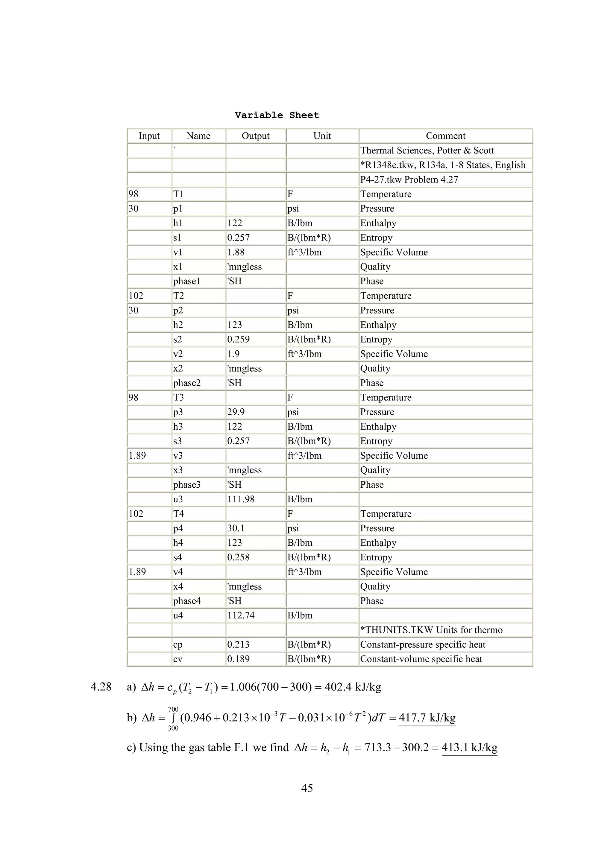
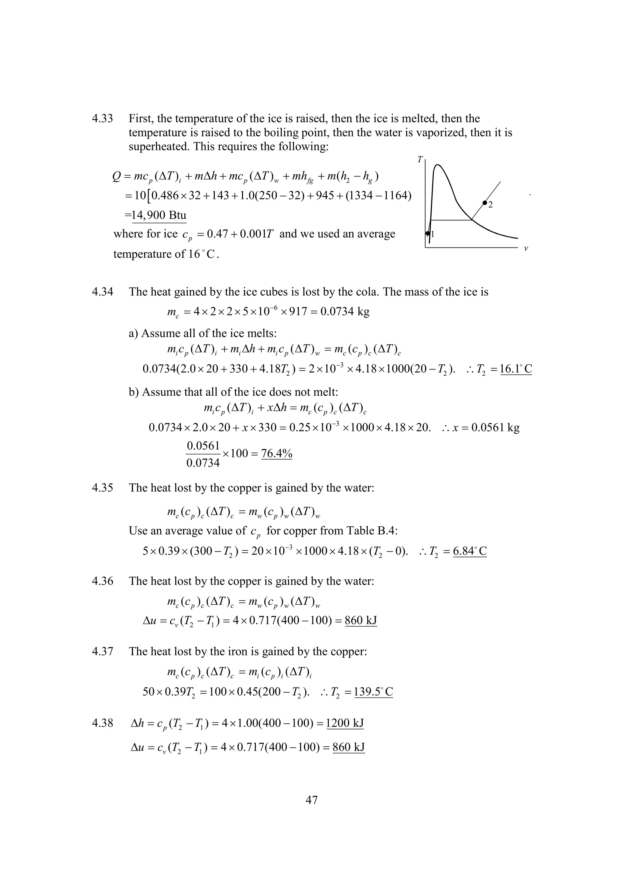
The document discusses various concepts and calculations related to the first law of thermodynamics, focusing on processes involving heat transfer, work, and internal energy changes in thermodynamic systems. It includes specific computations for adiabatic processes, superheated steam, and interpolations using thermodynamic tables. The calculations illustrate principles such as heat loss, energy conservation, and temperature changes in rigid containers under different conditions.
![Introduction to chemical engineering thermodynamics, 6th ed [solution]](https://cdn.slidesharecdn.com/ss_thumbnails/introductiontochemicalengineeringthermodynamics6thedsolution-160504021702-thumbnail.jpg?width=640&height=640&fit=bounds)


![[W f stoecker]_refrigeration_and_a_ir_conditioning_(book_zz.org)](https://cdn.slidesharecdn.com/ss_thumbnails/wfstoeckerrefrigerationandairconditioningbookzz-161019162540-thumbnail.jpg?width=640&height=640&fit=bounds)


![Coded Agents – with UiPath SDK + LangGraph [Virtual Hands-on Workshop]](https://cdn.slidesharecdn.com/ss_thumbnails/codedagentsdeck-251215155422-5497c599-thumbnail.jpg?width=640&height=640&fit=bounds)


