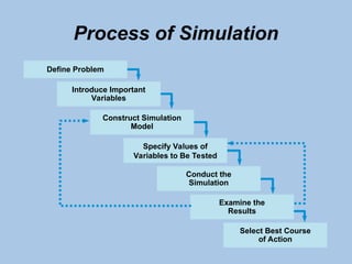
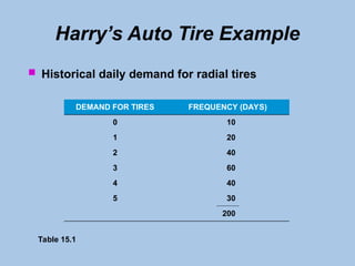
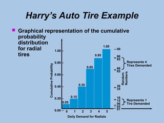
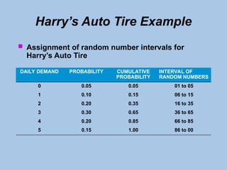
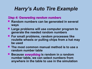
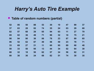
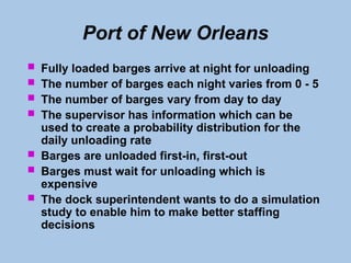
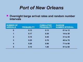
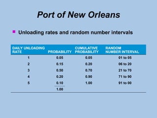
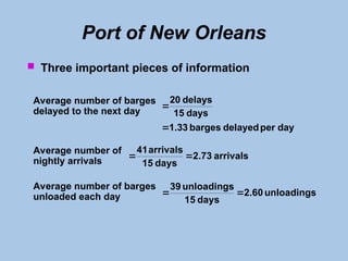
The document outlines the principles and processes of simulation modeling, focusing on its utility in analyzing complex real-world problems through a mathematical approach. It covers the seven steps of conducting a simulation, discusses advantages and disadvantages, and introduces the Monte Carlo method for handling probabilistic elements. Additionally, it presents practical examples, such as managing inventory at Harry's Auto Tire and simulating unloading operations at the Port of New Orleans.

1. Simulation Modeling

2. Learning Objectives
1. Tacke a wide variety of problems by
simulation
2. Understand the seven steps of conducting a
simulation
3. Explain the advantages and disadvantages of
simulation
4. Develop random number intervals and use
them to generate outcomes
After completing this chapter, students will be able to:
After completing this chapter, students will be able to:

3. Introduction
 Simulation
Simulation is one of the most widely used
quantitative analysis tools
 It is used by over half of the largest US
corporations in corporate planning
 To simulate
simulate is to try to duplicate the features,
appearance, and characteristics of a real system
 We will build a mathematical model
mathematical model that comes
as close as possible to representing the reality
of the system
 You can also build physical
physical models to test
systems

4. Introduction
 The idea behind simulation is to imitate a real-
world situation mathematically
 Study its properties and operating characteristics
 Draw conclusions and make action decisions

5. Introduction
 Using simulation, a manager should
1. Define a problem
2. Introduce the variables associated with the
problem
3. Construct a numerical model
4. Set up possible courses of action for testing
5. Run the experiment
6. Consider the results
7. Decide what courses of action to take

6. Process of Simulation
Define Problem
Introduce Important
Variables
Construct Simulation
Model
Specify Values of
Variables to Be Tested
Conduct the
Simulation
Examine the
Results
Select Best Course
of Action

7. Advantages and Disadvantages
of Simulation
 Simulation is useful because
1. It is relatively straightforward and flexible
2. Recent advances in computer software make
simulation models very easy to develop
3. Can be used to analyze large and complex
real-world situations
4. Allows “what-if?” type questions
5. Does not interfere with the real-world system
6. Enables study of interactions between
components
7. Enables time compression
8. Enables the inclusion of real-world
complications

8. Advantages and Disadvantages
of Simulation
 The main disadvantages of simulation are
1. It is often expensive as it may require a long,
complicated process to develop the model
2. Does not generate optimal solutions, it is a
trial-and-error approach
3. Requires managers to generate all conditions
and constraints of real-world problem
4. Each model is unique and the solutions and
inferences are not usually transferable to
other problems

9. Monte Carlo Simulation
 When systems contain elements that exhibit
chance in their behavior, the Monte Carlo method
of simulation can be applied
 Some examples are
1. Inventory demand
2. Lead time for inventory
3. Times between machine breakdowns
4. Times between arrivals
5. Service times
6. Times to complete project activities
7. Number of employees absent

10. Monte Carlo Simulation
 The basis of the Monte Carlo simulation is
experimentation on the probabilistic elements
through random sampling
 It is based on the following five steps
1. Setting up a probability distribution for
important variables
2. Building a cumulative probability distribution
for each variable
3. Establishing an interval of random numbers for
each variable
4. Generating random numbers
5. Actually simulating a series of trials

11. Harry’s Auto Tire Example
 A popular radial tire accounts for a large portion
of the sales at Harry’s Auto Tire
 Harry wishes to determine a policy for managing
this inventory
 He wants to simulate the daily demand for a
number of days
Step 1: Establishing probability distributions
Step 1: Establishing probability distributions
 One way to establish a probability distribution for
a given variable is to examine historical outcomes
 Managerial estimates based on judgment and
experience can also be used

12. Harry’s Auto Tire Example
 Historical daily demand for radial tires
DEMAND FOR TIRES FREQUENCY (DAYS)
0 10
1 20
2 40
3 60
4 40
5 30
200
Table 15.1

13. Harry’s Auto Tire Example
Step 2:
Step 2: Building a cumulative probability distribution
Building a cumulative probability distribution
for each variable
for each variable
 Converting from a regular probability to a
cumulative distribution is an easy job
 A cumulative probability is the probability that a
variable will be less than or equal to a particular
value
 A cumulative distribution lists all of the possible
values and the probabilities
 Tables below show these distributions

14. Harry’s Auto Tire Example
 Probability of demand for radial tires
DEMAND VARIABLE PROBABILITY OF OCCURRENCE
0 10/200 = 0.05
1 20/200 = 0.10
2 40/200 = 0.20
3 60/200 = 0.30
4 40/200 = 0.20
5 30/200 = 0.15
200/200 = 1.00

15. Harry’s Auto Tire Example
 Cumulative probability for radial tires
DAILY DEMAND PROBABILITY CUMULATIVE PROBABILITY
0 0.05 0.05
1 0.10 0.15
2 0.20 0.35
3 0.30 0.65
4 0.20 0.85
5 0.15 1.00

16. Harry’s Auto Tire Example
Step 3: Setting random number intervals
Step 3: Setting random number intervals
 We assign a set of numbers to represent each
possible value or outcome
 These are random number intervals
random number intervals
 A random number
random number is a series of digits that have
been selected by a totally random process
 The range of the random number intervals
corresponds exactly
exactly to the probability of the
outcomes as shown in Figure below

17. Harry’s Auto Tire Example
 Graphical representation of the cumulative
probability
distribution
for radial
tires
– 00
86
85
66
65
36
35
16
15
06
05
01
–
–
–
–
–
–
–
–
–
–
–
Random
Numbers
Represents 4
Tires Demanded
Represents 1
Tire Demanded
0.05
0.15
0.35
0.65
0.85
1.00
1.00 –
0.80 –
0.60 –
0.40 –
0.20 –
0.00 – 0 1 2 3 4 5
Daily Demand for Radials
Cumulative
Probability

18. Harry’s Auto Tire Example
 Assignment of random number intervals for
Harry’s Auto Tire
DAILY DEMAND PROBABILITY CUMULATIVE
PROBABILITY
INTERVAL OF
RANDOM NUMBERS
0 0.05 0.05 01 to 05
1 0.10 0.15 06 to 15
2 0.20 0.35 16 to 35
3 0.30 0.65 36 to 65
4 0.20 0.85 66 to 85
5 0.15 1.00 86 to 00

19. Harry’s Auto Tire Example
Step 4: Generating random numbers
Step 4: Generating random numbers
 Random numbers can be generated in several
ways
 Large problems will use computer program to
generate the needed random numbers
 For small problems, random processes like
roulette wheels or pulling chips from a hat may
be used
 The most common manual method is to use a
random number table
 Because everything
everything is random in a random
number table, we can select numbers from
anywhere in the table to use in the simulation

20. Harry’s Auto Tire Example
 Table of random numbers (partial)
52 06 50 88 53 30 10 47 99 37
37 63 28 02 74 35 24 03 29 60
82 57 68 28 05 94 03 11 27 79
69 02 36 49 71 99 32 10 75 21
98 94 90 36 06 78 23 67 89 85
96 52 62 87 49 56 59 23 78 71
33 69 27 21 11 60 95 89 68 48
50 33 50 95 13 44 34 62 64 39
88 32 18 50 62 57 34 56 62 31
90 30 36 24 69 82 51 74 30 35

21. Harry’s Auto Tire Example
Step 5: Simulating the experiment
Step 5: Simulating the experiment
 We select random numbers from Table 15.5
 The number we select will have a corresponding
range in Table 15.4
 We use the daily demand that corresponds to the
probability range aligned with the random
number

22. Harry’s Auto Tire Example
 Ten-day simulation of demand for radial tires
DAY RANDOM NUMBER SIMULATED DAILY DEMAND
1 52 3
2 37 3
3 82 4
4 69 4
5 98 5
6 96 5
7 33 2
8 50 3
9 88 5
10 90 5
39 = total 10-day demand
3.9 = average daily demand for tires

23. Harry’s Auto Tire Example
 Note that the average demand from this
simulation (3.9 tires) is different from the
expected
expected daily demand
Expected
daily
demand
  
tires
of
Demand
tires
of
y
Probabilit
5
0
i
i
i



 (0.05)(0) + (0.10)(1) + (0.20)(2) + (0.30)(3)
+ (0.20)(4) + (0.15)(5)
 2.95 tires
 If this simulation were repeated hundreds or
thousands of times it is much more likely the
average simulated
simulated demand would be nearly the
same as the expected
expected demand

24. Simulation of a Queuing Problem
 Modeling waiting lines is an important application
of simulation
 The assumptions of queuing models are quite
restrictive
 Sometimes simulation is the only approach that
fits
 In this example, arrivals do not follow a Poisson
distribution and unloading rates are not
exponential or constant

25. Port of New Orleans
 Fully loaded barges arrive at night for unloading
 The number of barges each night varies from 0 - 5
 The number of barges vary from day to day
 The supervisor has information which can be
used to create a probability distribution for the
daily unloading rate
 Barges are unloaded first-in, first-out
 Barges must wait for unloading which is
expensive
 The dock superintendent wants to do a simulation
study to enable him to make better staffing
decisions

26. Port of New Orleans
 Overnight barge arrival rates and random number
intervals
NUMBER OF
ARRIVALS PROBABILITY
CUMULATIVE
PROBABILITY
RANDOM
NUMBER INTERVAL
0 0.13 0.13 01 to 13
1 0.17 0.30 14 to 30
2 0.15 0.45 31 to 45
3 0.25 0.70 46 to 70
4 0.20 0.90 71 to 90
5 0.10 1.00 91 to 00

27. Port of New Orleans
 Unloading rates and random number intervals
DAILY UNLOADING
RATE PROBABILITY
CUMULATIVE
PROBABILITY
RANDOM
NUMBER INTERVAL
1 0.05 0.05 01 to 05
2 0.15 0.20 06 to 20
3 0.50 0.70 21 to 70
4 0.20 0.90 71 to 90
5 0.10 1.00 91 to 00
1.00

28. Port of New Orleans
 Queuing simulation of barge unloadings
(1)
DAY
(2)
NUMBER DELAYED
FROM PREVIOUS DAY
(3)
RANDOM
NUMBER
(4)
NUMBER OF
NIGHTLY ARRIVALS
(5)
TOTAL TO BE
UNLOADED
(6)
RANDOM
NUMBER
(7)
NUMBER
UNLOADED
1 — 52 3 3 37 3
2 0 06 0 0 63 0
3 0 50 3 3 28 3
4 0 88 4 4 02 1
5 3 53 3 6 74 4
6 2 30 1 3 35 3
7 0 10 0 0 24 0
8 0 47 3 3 03 1
9 2 99 5 7 29 3
10 4 37 2 6 60 3
11 3 66 3 6 74 4
12 2 91 5 7 85 4
13 3 35 2 5 90 4
14 1 32 2 3 73 3
15 0 00 5 5 59 3
20 41 39
Total delays Total arrivals Total unloadings

29. Port of New Orleans
 Three important pieces of information
Average number of barges
delayed to the next day
day
per
delayed
barges
1.33
days
15
delays
20


Average number of
nightly arrivals
arrivals
2.73
days
15
arrivals
41


Average number of barges
unloaded each day unloadings
2.60
days
15
unloadings
39

