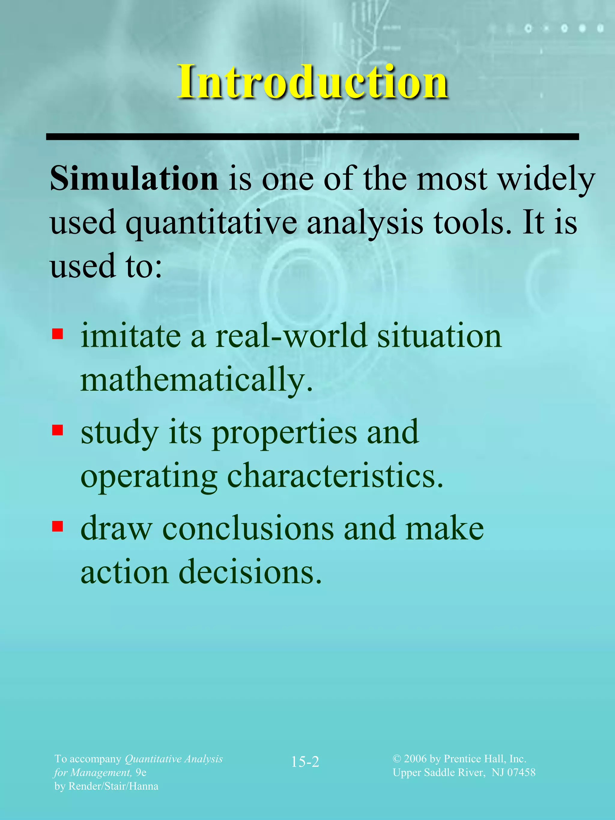
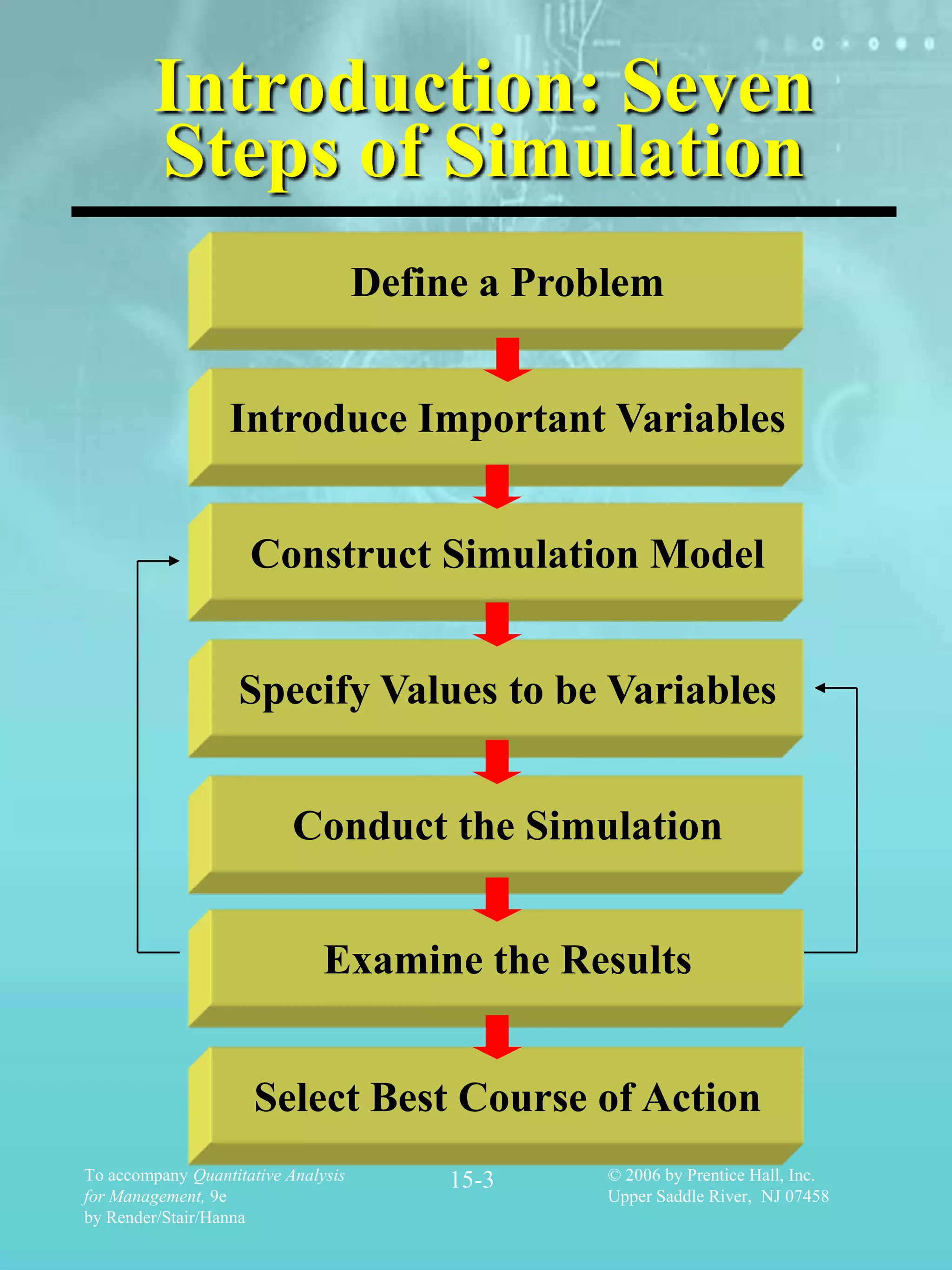
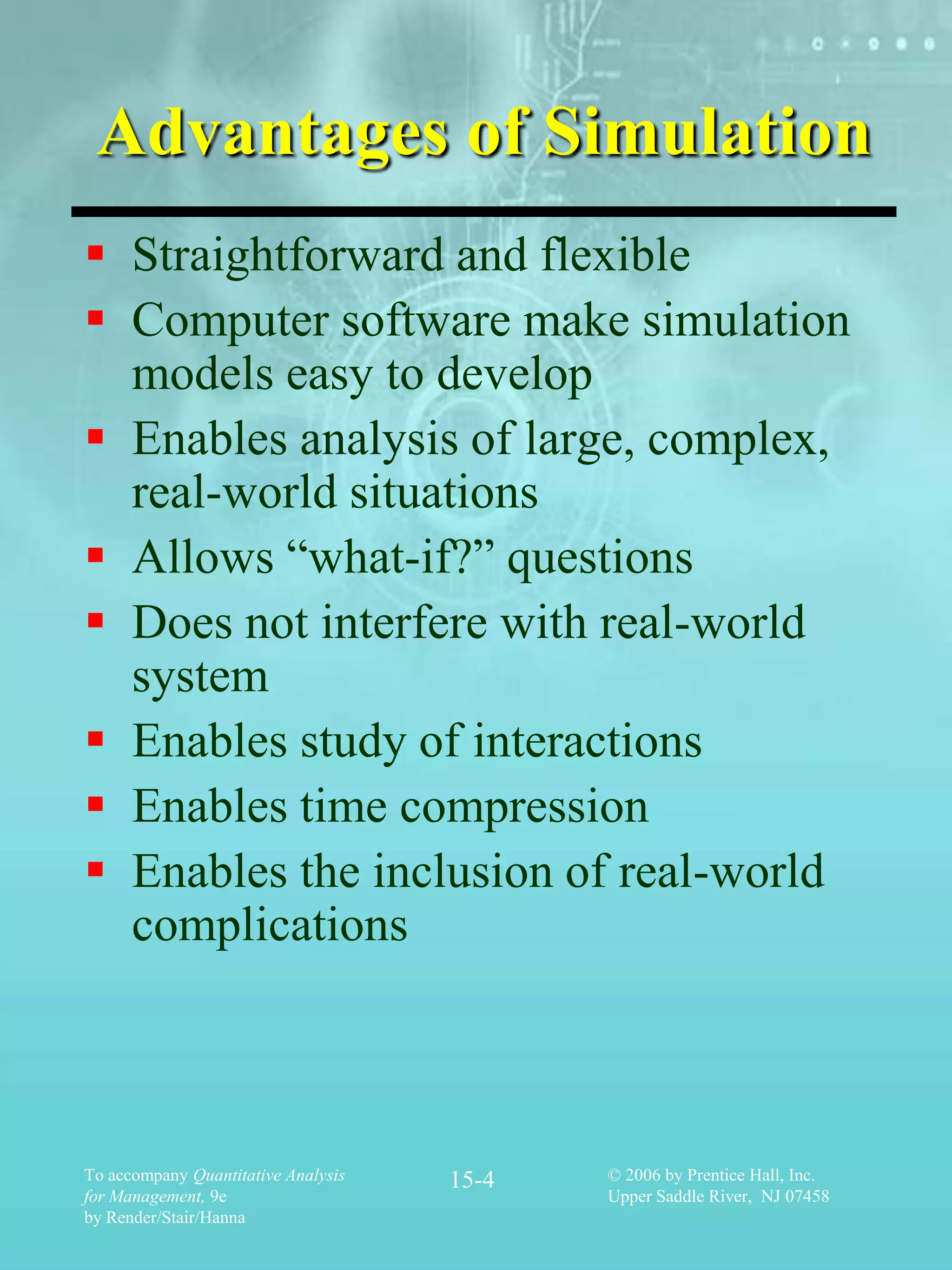
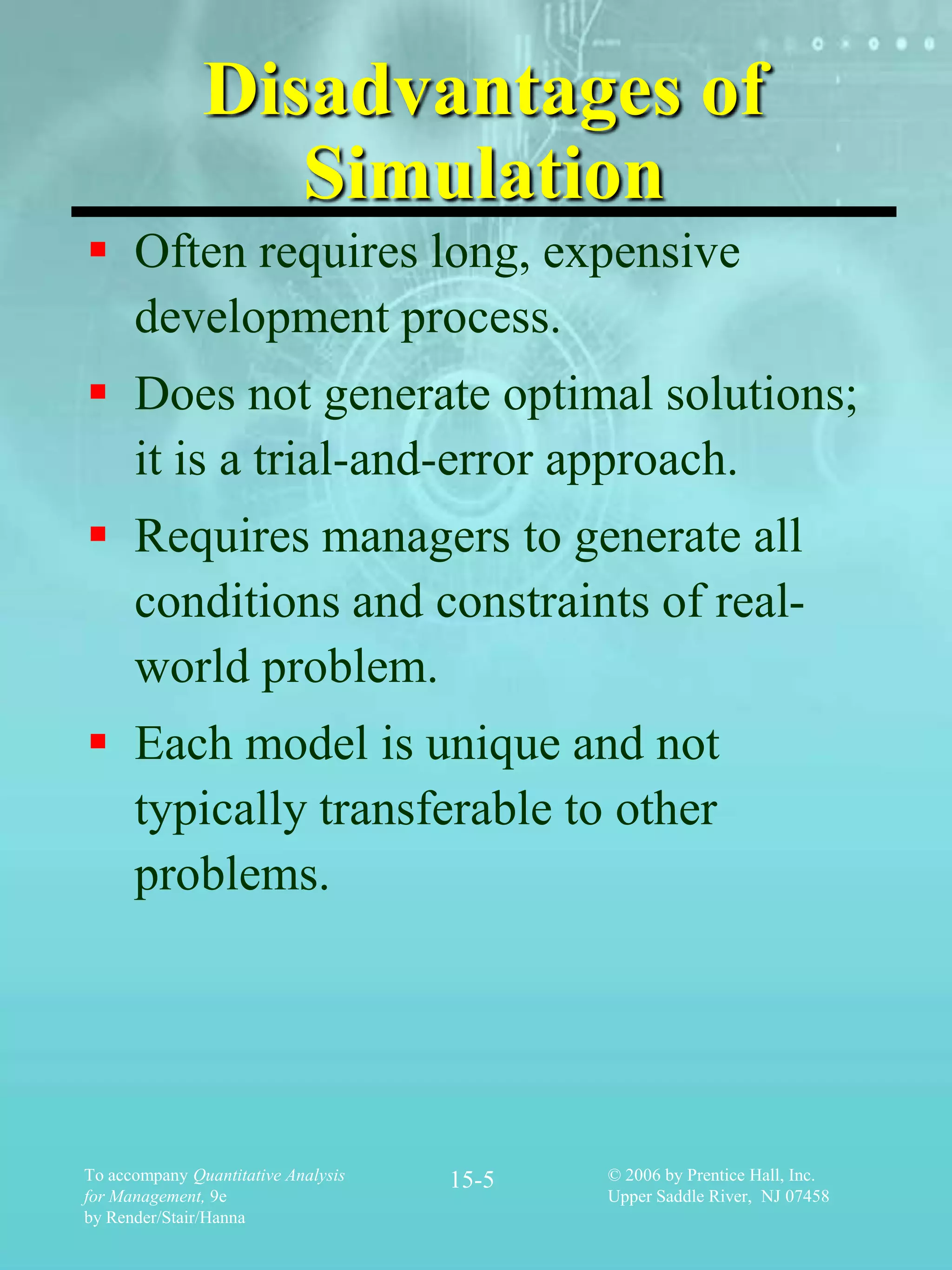
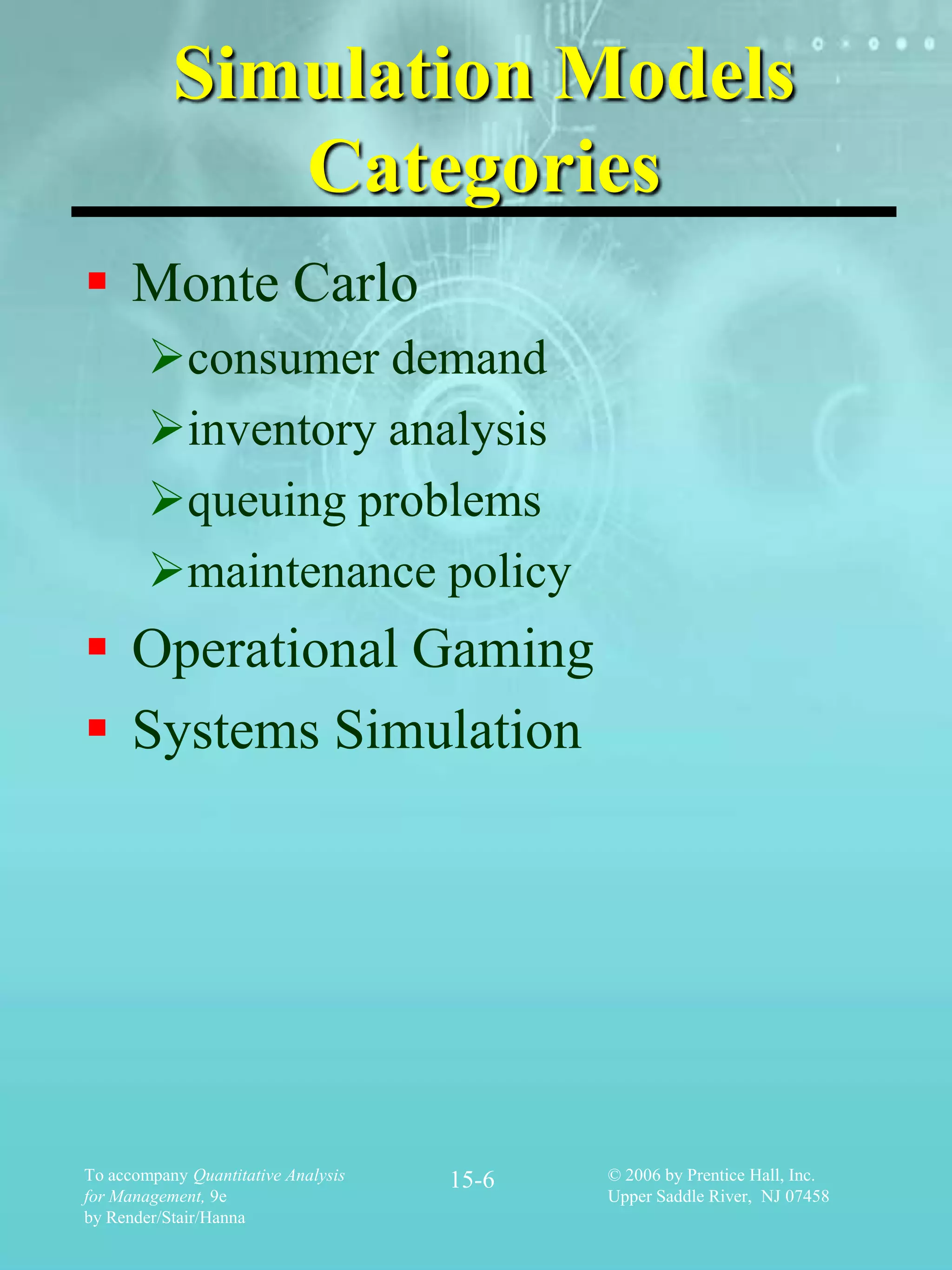
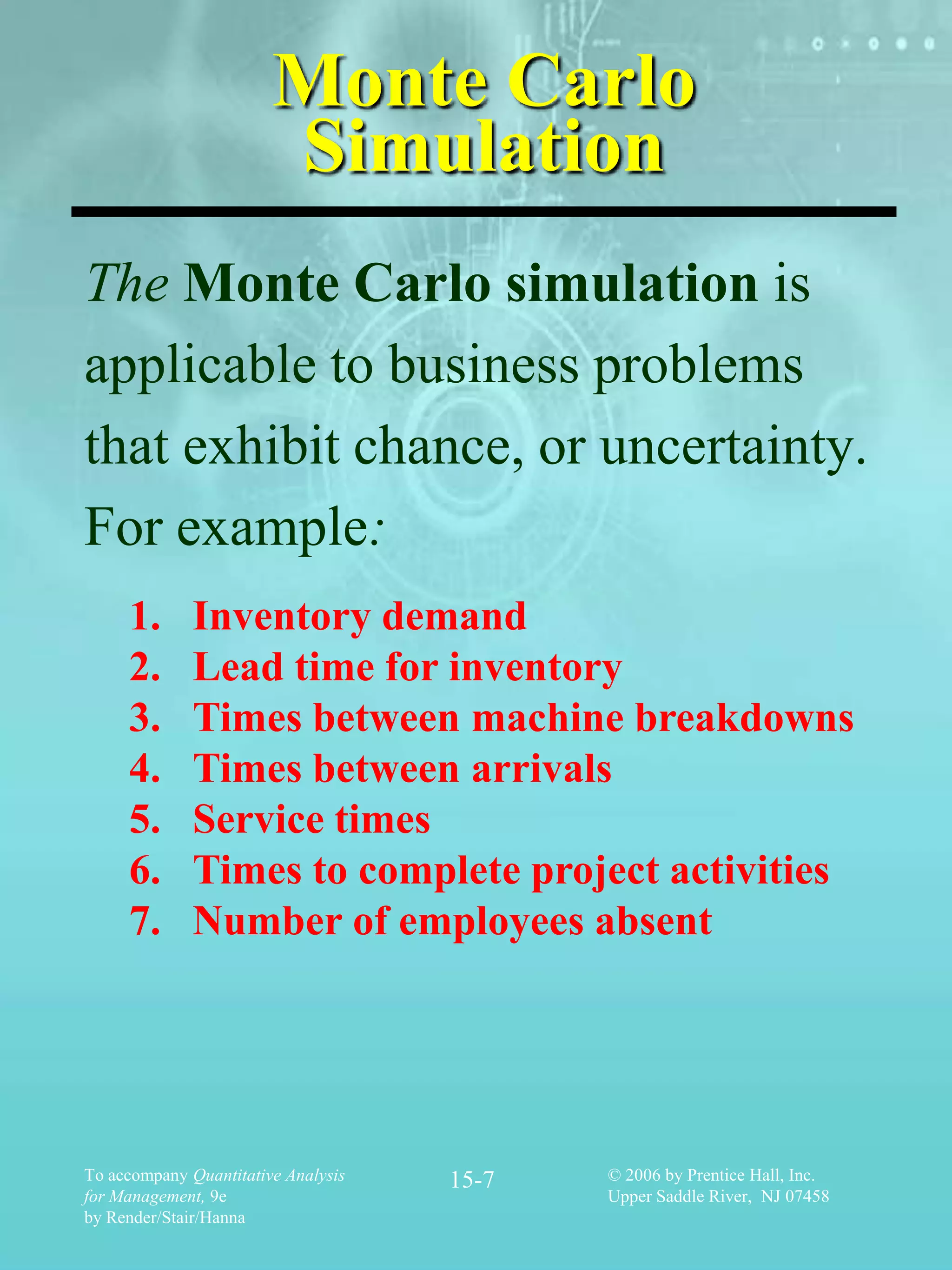
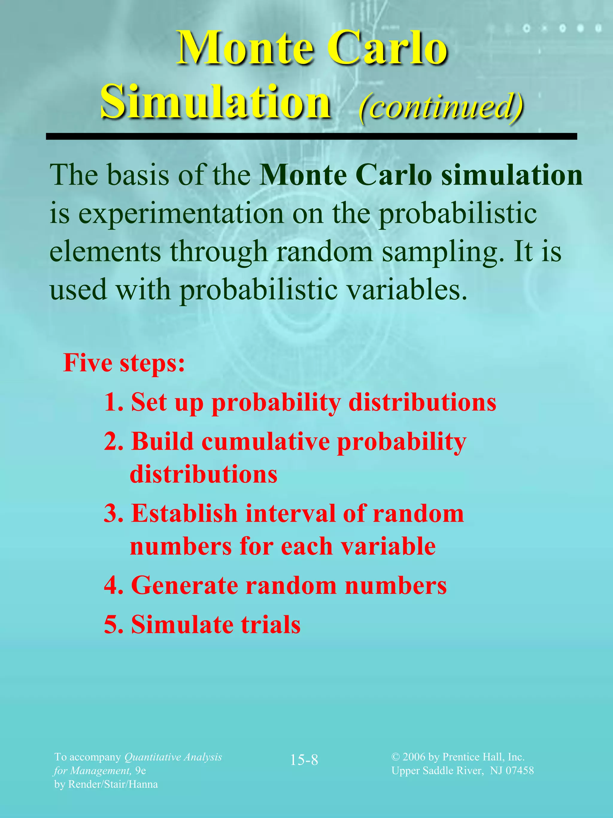
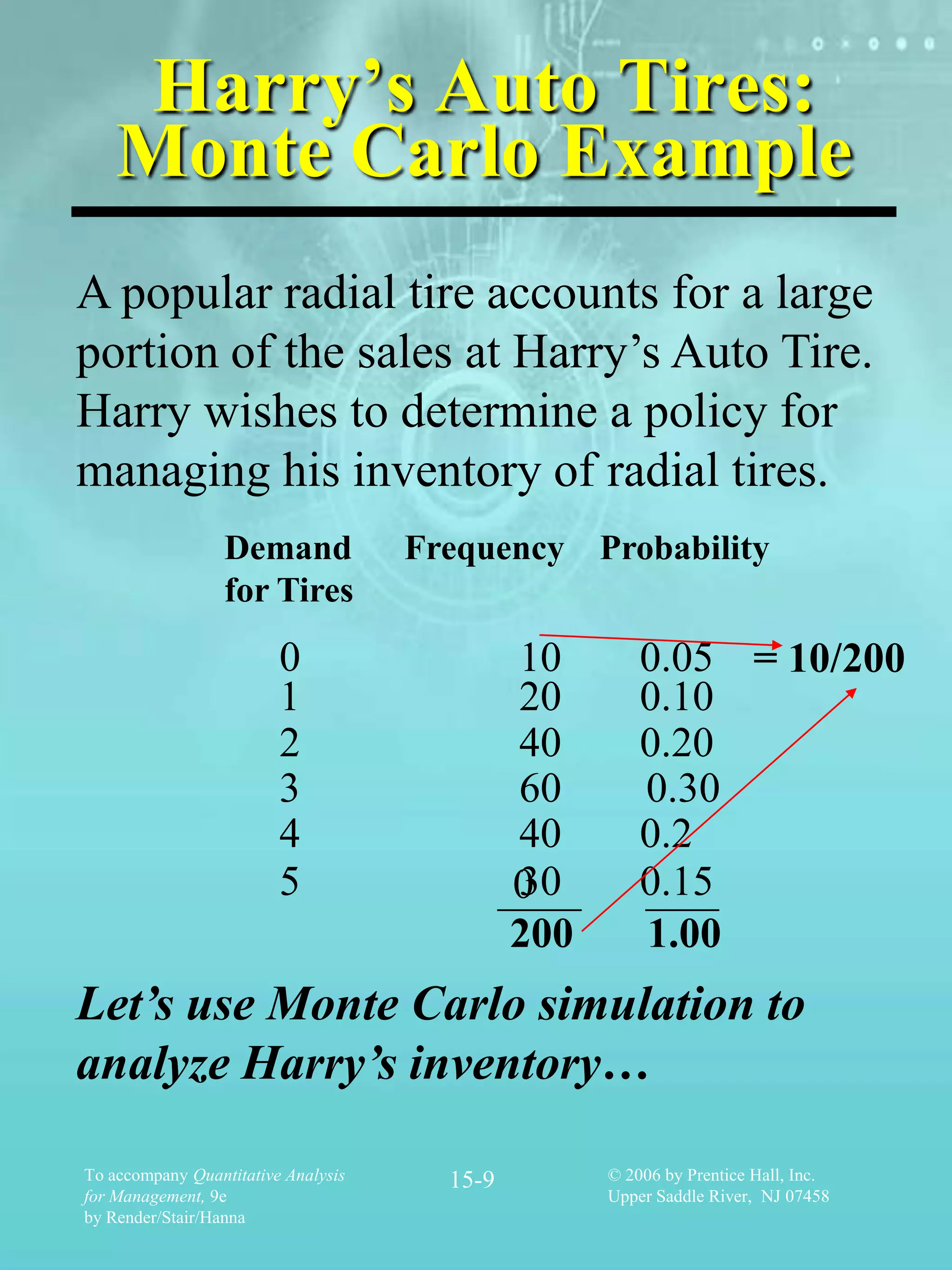
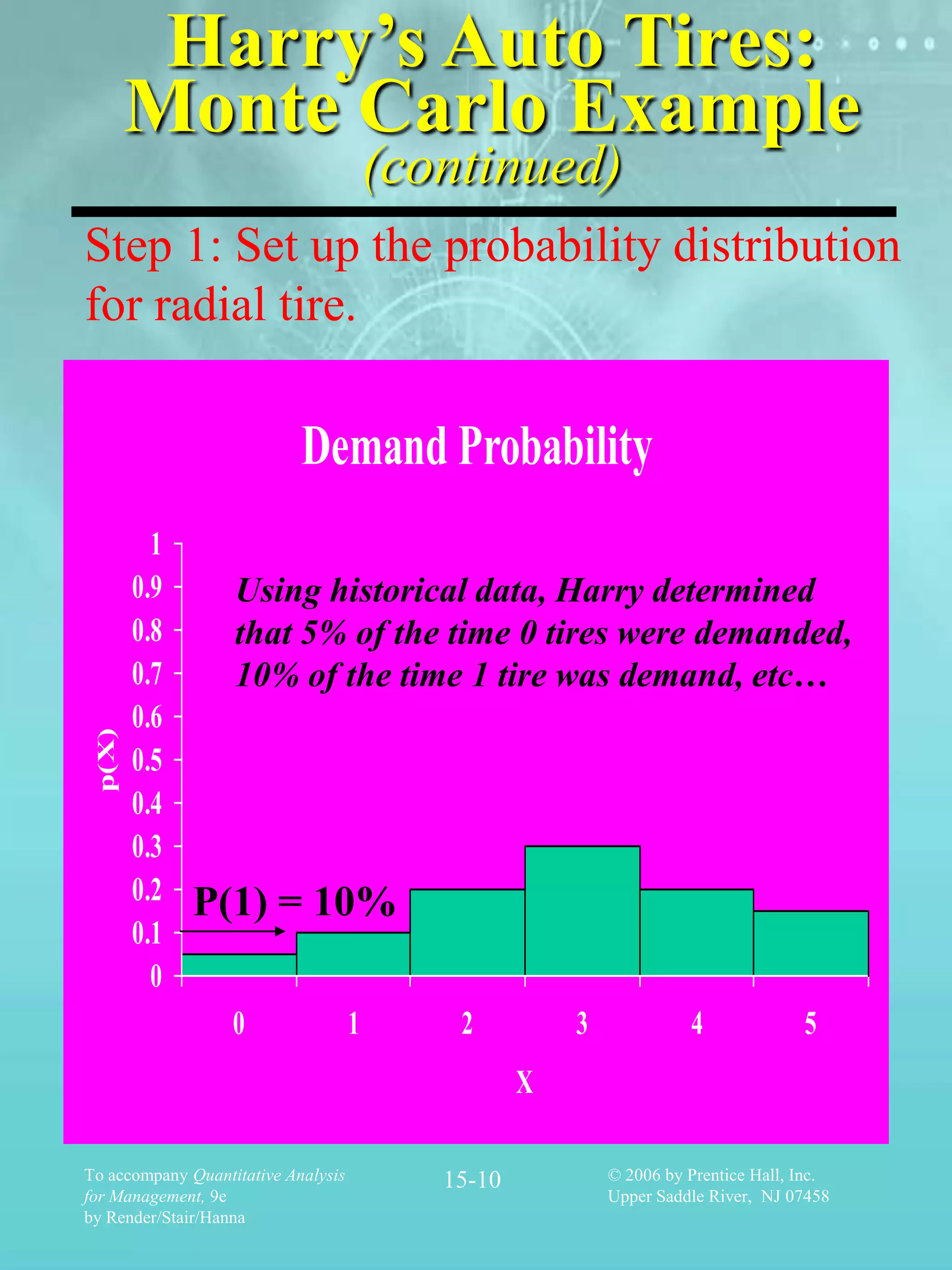
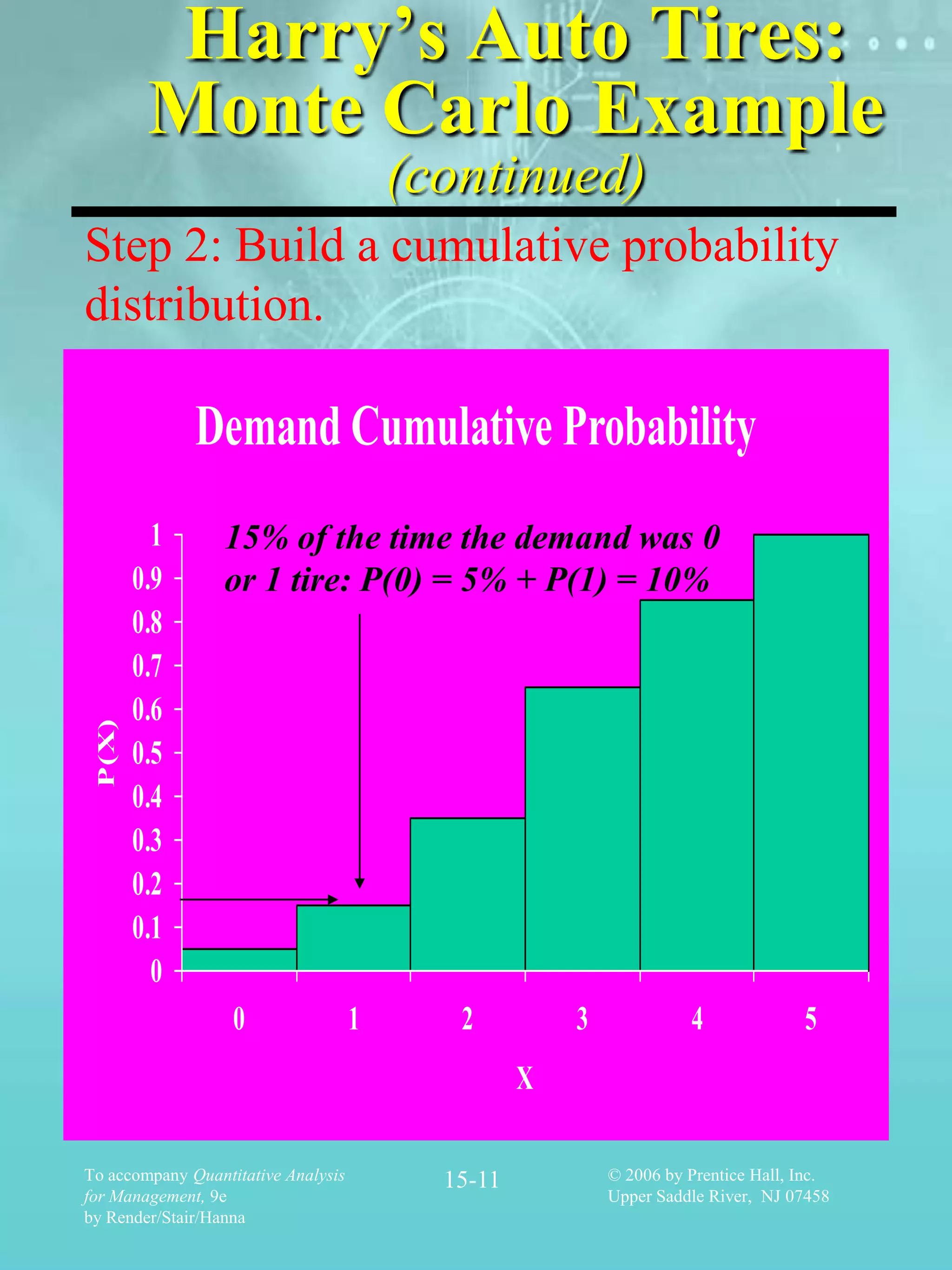
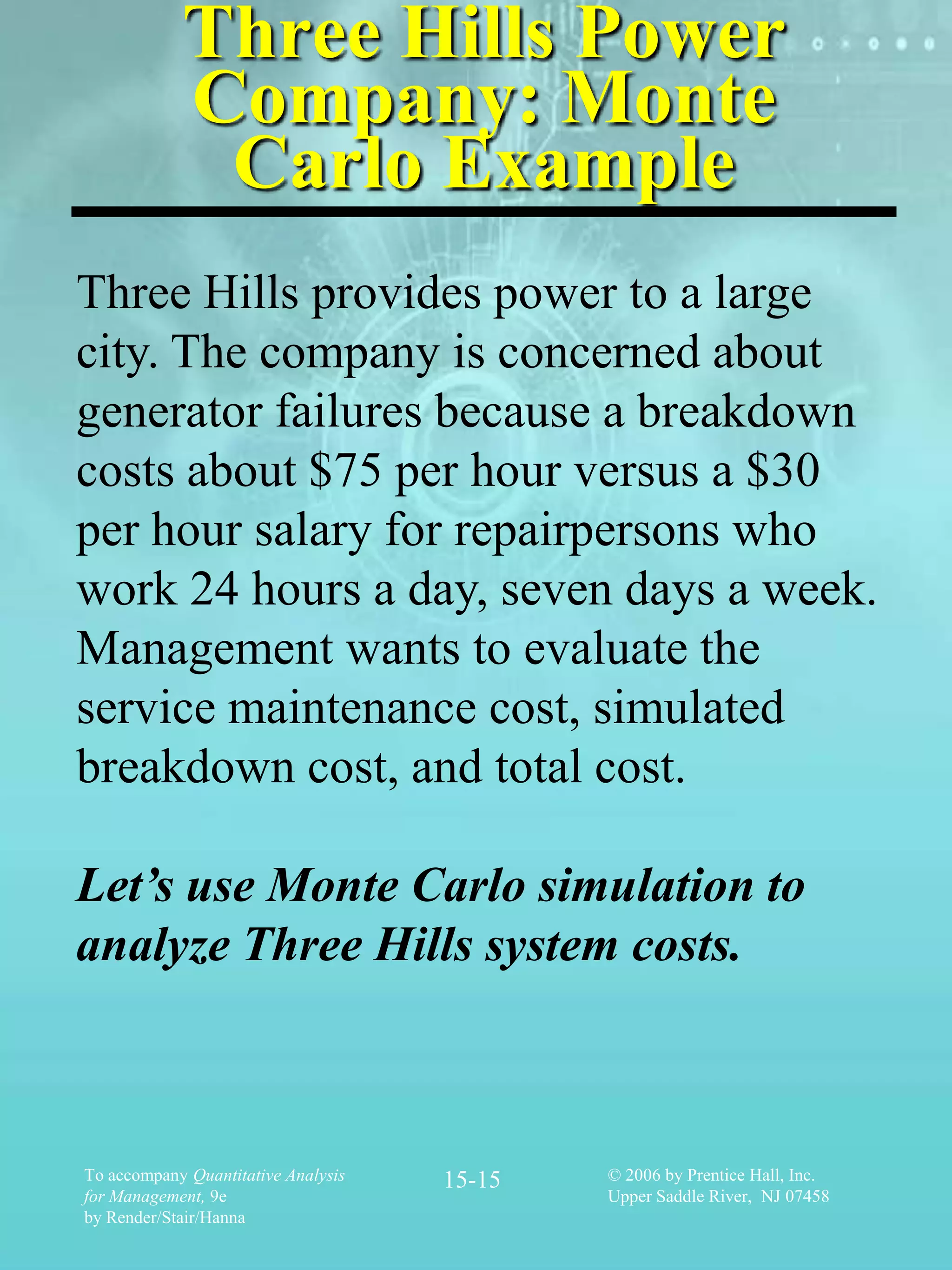
SlideShare a Scribd company logo
1 of 22
Simulation
                   Modeling


               Prepared by Lee Revere and John Large
To accompany Quantitative Analysis   15-1   © 2006 by Prentice Hall, Inc.
for Management, 9e                          Upper Saddle River, NJ 07458
by Render/Stair/Hanna
Introduction
Simulation is one of the most widely
used quantitative analysis tools. It is
used to:
 imitate a real-world situation
  mathematically.
 study its properties and
  operating characteristics.
 draw conclusions and make
  action decisions.


To accompany Quantitative Analysis   15-2   © 2006 by Prentice Hall, Inc.
for Management, 9e                          Upper Saddle River, NJ 07458
by Render/Stair/Hanna
Introduction: Seven
        Steps of Simulation
                                     Define a Problem


                  Introduce Important Variables


                     Construct Simulation Model


                    Specify Values to be Variables


                           Conduct the Simulation


                               Examine the Results


                      Select Best Course of Action
To accompany Quantitative Analysis        15-3    © 2006 by Prentice Hall, Inc.
for Management, 9e                                Upper Saddle River, NJ 07458
by Render/Stair/Hanna
Advantages of Simulation
 Straightforward and flexible
 Computer software make simulation
  models easy to develop
 Enables analysis of large, complex,
  real-world situations
 Allows “what-if?” questions
 Does not interfere with real-world
  system
 Enables study of interactions
 Enables time compression
 Enables the inclusion of real-world
  complications


To accompany Quantitative Analysis   15-4   © 2006 by Prentice Hall, Inc.
for Management, 9e                          Upper Saddle River, NJ 07458
by Render/Stair/Hanna
Disadvantages of
                  Simulation
 Often requires long, expensive
  development process.
 Does not generate optimal solutions;
  it is a trial-and-error approach.
 Requires managers to generate all
  conditions and constraints of real-
  world problem.
 Each model is unique and not
  typically transferable to other
  problems.


To accompany Quantitative Analysis   15-5   © 2006 by Prentice Hall, Inc.
for Management, 9e                          Upper Saddle River, NJ 07458
by Render/Stair/Hanna
Simulation Models
              Categories
 Monte Carlo
        consumer demand
        inventory analysis
        queuing problems
        maintenance policy
 Operational Gaming
 Systems Simulation


To accompany Quantitative Analysis   15-6   © 2006 by Prentice Hall, Inc.
for Management, 9e                          Upper Saddle River, NJ 07458
by Render/Stair/Hanna
Monte Carlo
                        Simulation
The Monte Carlo simulation is
applicable to business problems
that exhibit chance, or uncertainty.
For example:
     1.       Inventory demand
     2.       Lead time for inventory
     3.       Times between machine breakdowns
     4.       Times between arrivals
     5.       Service times
     6.       Times to complete project activities
     7.       Number of employees absent


To accompany Quantitative Analysis   15-7   © 2006 by Prentice Hall, Inc.
for Management, 9e                          Upper Saddle River, NJ 07458
by Render/Stair/Hanna
Monte Carlo
        Simulation (continued)
The basis of the Monte Carlo simulation
is experimentation on the probabilistic
elements through random sampling. It is
used with probabilistic variables.

 Five steps:
    1. Set up probability distributions
    2. Build cumulative probability
       distributions
    3. Establish interval of random
       numbers for each variable
    4. Generate random numbers
    5. Simulate trials


To accompany Quantitative Analysis   15-8   © 2006 by Prentice Hall, Inc.
for Management, 9e                          Upper Saddle River, NJ 07458
by Render/Stair/Hanna
Harry’s Auto Tires:
    Monte Carlo Example
A popular radial tire accounts for a large
portion of the sales at Harry’s Auto Tire.
Harry wishes to determine a policy for
managing his inventory of radial tires.
                  Demand             Frequency Probability
                  for Tires
                         0                    10        0.05 = 10/200
                         1                    20        0.10
                         2                    40        0.20
                         3                    60        0.30
                         4                    40        0.2
                         5                    30
                                              0         0.15
                                              200       1.00
Let’s use Monte Carlo simulation to
analyze Harry’s inventory…

To accompany Quantitative Analysis     15-9         © 2006 by Prentice Hall, Inc.
for Management, 9e                                  Upper Saddle River, NJ 07458
by Render/Stair/Hanna
Harry’s Auto Tires:
        Monte Carlo Example
                                         (continued)
Step 1: Set up the probability distribution
for radial tire.

                            Demand Probability
          1
        0.9        Using historical data, Harry determined
        0.8        that 5% of the time 0 tires were demanded,
        0.7        10% of the time 1 tire was demand, etc…
        0.6
 p(X)


        0.5
        0.4
        0.3
        0.2   P(1) = 10%
        0.1
          0
                   0                 1       2          3             4              5
                                                    X

To accompany Quantitative Analysis          15-10           © 2006 by Prentice Hall, Inc.
for Management, 9e                                          Upper Saddle River, NJ 07458
by Render/Stair/Hanna
Harry’s Auto Tires:
         Monte Carlo Example
                                         (continued)
Step 2: Build a cumulative probability
distribution.

              Demand Cumulative Probability
          1       15% of the time the demand was 0
        0.9       or 1 tire: P(0) = 5% + P(1) = 10%
        0.8
        0.7
        0.6
 P(X)


        0.5
        0.4
        0.3
        0.2
        0.1
          0
                   0                 1      2          3             4              5
                                                   X

To accompany Quantitative Analysis         15-11           © 2006 by Prentice Hall, Inc.
for Management, 9e                                         Upper Saddle River, NJ 07458
by Render/Stair/Hanna
Harry’s Auto Tires: Monte
    Carlo Example (continued)
  Step 3: Establish an interval of random
  numbers.

                                        Probability


                                                                              Random
         Demand


                                                                              Number
                                                                              Interval
                                                                                                 Must be in correct proportion
         0              10             0.05                   0.05             01 - 05
         1              20             0.10                   0.15             06 - 15
         2              40             0.20                   0.35             16 - 35
         3              60             0.30                   0.65             36 - 65
         4              40             0.20                   0.85             66 - 85
         5              30             0.15                   1.00             86 - 00
Note: 5% of the time 0 tires are demanded, so the random
number interval contains 5% of the numbers between 1 and 100
  To accompany Quantitative Analysis                  15-12      © 2006 by Prentice Hall, Inc.
  for Management, 9e                                             Upper Saddle River, NJ 07458
  by Render/Stair/Hanna
Harry’s Auto Tires: Monte
 Carlo Example (continued)
 Step 4: Generate random numbers.
 52   06    50 88     53    30        10   47   99   37 66   91 35    32    00    84    57 07
 37   63    28 02     74    35        24   03   29   60 74   85 90    73    59    55    17 60
 82   57    68 28     05    94        03   11   27   79 90   87 92    41    09    25    36 77
 69   02    36 49     71    99        32   10   75   21 95   90 94    38    97    71    72 49
 98   94    90 36     06    78        23   67   89   85 29   21 25    73    69    34    85 76
 96   52    62 87     49    56        59   23   78   71 72   90 57    01    98    57    31 95
 33   69    27 21     11    60        95   89   68   48 17   89 34    09    93    50    44 51
 50   33    50 95     13    44        34   62   64   39 55   29 30    64    49    44    30 16
 88   32    18 50     62    57        34   56   62   31 15   40 90    34    51    95    26 14
 90   30    36 24     69    82        51   74   30   35 36   85 01    55    92    64    09 85
 50   48    61 18     85    23        08   54   17   12 80   69 24    84    92    16    49 59
 27   88    21 62     69    64        48   31   12   73 02   68 00    16    16    46    13 85
 45   14    46 32     13    49        66   62   74   41 86   98 92    98    84    54    33 40
 81   02    01 78     82    74        97   37   45   31 94   99 42    49    27    64    89 42
 66   83    14 74     27    76        03   33   11   97 59   81 72    00    64    61    13 52
 74   05    82 82     93    09        96   33   52   78 13   06 28    30    94    23    37 39
 30   34    87 01     74    11        46   82   59   94 25   34 32    23    17    01    58 73


 To accompany Quantitative Analysis             15-13         © 2006 by Prentice Hall, Inc.
 for Management, 9e                                           Upper Saddle River, NJ 07458
 by Render/Stair/Hanna
Harry’s Auto Tires: Monte
 Carlo Example (continued)
   Step 5: Simulate a series of trials.
   Using random number table on previous slide,
   simulated demand for 10 days is:

         Tires                                      Interval of
         Demanded                                   Random Numbers

         0                                          01 - 05
         1                                          06 - 15
         2                                          16 - 35
         3                     2                    36 - 65
         4                                          66 - 85
         5             3                1           86 - 100

Random number: 52 06 50 88 53 30 10 47 99 37
Simulated demand: 3 1 3 5 3 2 1 3 5 3


   To accompany Quantitative Analysis       15-14        © 2006 by Prentice Hall, Inc.
   for Management, 9e                                    Upper Saddle River, NJ 07458
   by Render/Stair/Hanna
Three Hills Power
            Company: Monte
             Carlo Example
Three Hills provides power to a large
city. The company is concerned about
generator failures because a breakdown
costs about $75 per hour versus a $30
per hour salary for repairpersons who
work 24 hours a day, seven days a week.
Management wants to evaluate the
service maintenance cost, simulated
breakdown cost, and total cost.

Let’s use Monte Carlo simulation to
analyze Three Hills system costs.


To accompany Quantitative Analysis   15-15   © 2006 by Prentice Hall, Inc.
for Management, 9e                           Upper Saddle River, NJ 07458
by Render/Stair/Hanna
Three Hills Power
Generator Breakdown Times:
   Monte Carlo (continued)
 Steps 1-3: Determine probability,
 cumulative probability, and random
 number interval - BREAKDOWNS.


                                                                       Random Number
                        Times Observed
                          Number of


                                                                           Interval
                                                 Cumulative
                                                 Probability


      ½                        5         0.05      0.05                01 - 05
     1                        6          0.06      0.11                06 - 11
    1½                       16          0.16      0.27                12 - 27
      2                      33          0.33      0.60                28 - 60
    2½                       21          0.21      0.81                81 - 81
     3                       19          0.19      1.00                82 - 00
 Total                     100           1.00
 To accompany Quantitative Analysis      15-16   © 2006 by Prentice Hall, Inc.
 for Management, 9e                              Upper Saddle River, NJ 07458
 by Render/Stair/Hanna
Three Hills Power
            Generator Repair
                 Times
Steps 1-3: Determine probability,
cumulative probability, and random
number interval - REPAIRS.
Repair Time


                                               Cumulative
 Required


                                               Probability
  (Hours)


   1                 28              0.28      0.28            01 - 28


   2                 52              0.52      0.80            29 - 80


   3                  20             0.20      1.00            81 - 00
To accompany Quantitative Analysis     15-17     © 2006 by Prentice Hall, Inc.
for Management, 9e                               Upper Saddle River, NJ 07458
by Render/Stair/Hanna
Three Hills Power
Generator Breakdown Times:
   Monte Carlo (continued)
Steps 4 & 5: Generate random numbers and simulate.


                                                                                                               Machine is down
                                                   Time Repair


                                                                                                Time Repair
                                                                              Repair Time
                         Breakdowns


                                       Breakdown
 Simulation


                                                   Can Begin


                                                                                                               No. of hrs.
              Random


                                                                 Random
                         Time b/t
              Number


                                                                 Number
                                       Time of


                                                                                                Ends
 Trial


   1           57           2          2:00         2:00           7                  1         3:00            1

   2           17       1.5            3:30         3:30         60                   2         5:30            2

   3           36           2          5:30         5:30         77                   2         7:30            2

   4           72       2.5            8:00         8:00         49                   2 10:00                   2

   5           85           3         11:00        11:00         76                   2 13:00                   2

     :           :           :               :               :      :                       :            :       :

 14            89           3          4:00         6:00         42                   2         8:00            4

 15            13       1.5            5:30         8:00         52                   2 10:00                 4.5


      To accompany Quantitative Analysis           15-18                © 2006 by Prentice Hall, Inc.
      for Management, 9e                                                Upper Saddle River, NJ 07458
      by Render/Stair/Hanna
Three Hills Power
Generator Breakdown Times:
   Monte Carlo (continued)
 Cost Analysis:
 Service maintenance: = 34 hrs of worker
                         service X $30 per hr
                      = $1,020


Simulate machine breakdown costs:
                = 44 total hrs of breakdown
                X $75 lost per hr of downtime
                = $3,300

Total simulated maintenance cost of the
current system: = service cost + breakdown costs
                = $1,020 + $3,300
                = $4,320

 To accompany Quantitative Analysis   15-19   © 2006 by Prentice Hall, Inc.
 for Management, 9e                           Upper Saddle River, NJ 07458
 by Render/Stair/Hanna
Operational Gaming
        Simulation Model
Operational gaming refers to
simulation involving competing
players.

Examples:
    Military games
    Business games


To accompany Quantitative Analysis   15-20   © 2006 by Prentice Hall, Inc.
for Management, 9e                           Upper Saddle River, NJ 07458
by Render/Stair/Hanna
Systems Simulation
                Model
Systems simulation is similar to
business gaming because it allows
users to test various managerial
policies and decision. It models the
dynamics of large systems.

Examples:
 Corporate operating system
 Urban government
 Economic systems


To accompany Quantitative Analysis   15-21   © 2006 by Prentice Hall, Inc.
for Management, 9e                           Upper Saddle River, NJ 07458
by Render/Stair/Hanna
Verification and
                  Validation
Verification of simulation models
involves determining that the
computer model is internally
consistent and follows the logic of
the conceptual model.

Validation is the process of
comparing a simulation model
to a real system to assure
accuracy.


To accompany Quantitative Analysis   15-22   © 2006 by Prentice Hall, Inc.
for Management, 9e                           Upper Saddle River, NJ 07458
by Render/Stair/Hanna

More Related Content

What's hot

Merton Truck Company
Merton Truck CompanyMerton Truck Company
Merton Truck CompanyTushar Arora
 
Goodyear Aquatred Case Study - Marketing
Goodyear Aquatred Case Study - MarketingGoodyear Aquatred Case Study - Marketing
Goodyear Aquatred Case Study - MarketingMaria Medvedeva
 
Southwest Airlines in Baltimore
Southwest Airlines in BaltimoreSouthwest Airlines in Baltimore
Southwest Airlines in BaltimorePutri Arinda
 
Wal-Mart Stores’ Discount operations
Wal-Mart Stores’ Discount operationsWal-Mart Stores’ Discount operations
Wal-Mart Stores’ Discount operationsAJAL A J
 
ACME or OMEGA - case analysis
ACME or OMEGA - case analysis ACME or OMEGA - case analysis
ACME or OMEGA - case analysis Akhilesh Krishnan
 
Littlefield Simulation
Littlefield Simulation Littlefield Simulation
Littlefield Simulation Kamal Gelya
 
Waiting Lines & Simulation
Waiting Lines & SimulationWaiting Lines & Simulation
Waiting Lines & SimulationNavitha Pereira
 
Wilkerson Company Case
Wilkerson Company CaseWilkerson Company Case
Wilkerson Company CaseElla Shen
 
Harrah's Entertainment, Inc. Case Analysis
Harrah's Entertainment, Inc. Case AnalysisHarrah's Entertainment, Inc. Case Analysis
Harrah's Entertainment, Inc. Case Analysismbartugs
 
Bba 3274 qm week 9 transportation and assignment models
Bba 3274 qm week 9 transportation and assignment modelsBba 3274 qm week 9 transportation and assignment models
Bba 3274 qm week 9 transportation and assignment modelsStephen Ong
 
Cola Wars - Coke Vs Pepsi Harvard Business School Case Study
Cola Wars - Coke Vs Pepsi Harvard Business School Case StudyCola Wars - Coke Vs Pepsi Harvard Business School Case Study
Cola Wars - Coke Vs Pepsi Harvard Business School Case StudyMohan Kanni
 
CASE STUDY : The Treadway Tire Company
CASE STUDY : The Treadway Tire CompanyCASE STUDY : The Treadway Tire Company
CASE STUDY : The Treadway Tire CompanyTanya Taneja
 
HARLEY DAVIDSON CASE STUDY SOLUTION
HARLEY DAVIDSON CASE STUDY SOLUTIONHARLEY DAVIDSON CASE STUDY SOLUTION
HARLEY DAVIDSON CASE STUDY SOLUTIONfarouq umar
 

What's hot (20)

Merton Truck Company
Merton Truck CompanyMerton Truck Company
Merton Truck Company
 
Goodyear Aquatred Case Study - Marketing
Goodyear Aquatred Case Study - MarketingGoodyear Aquatred Case Study - Marketing
Goodyear Aquatred Case Study - Marketing
 
Acme and omega
Acme and omegaAcme and omega
Acme and omega
 
7 cemex (uneditted)
7 cemex (uneditted)7 cemex (uneditted)
7 cemex (uneditted)
 
Queueing theory
Queueing theoryQueueing theory
Queueing theory
 
Southwest Airlines in Baltimore
Southwest Airlines in BaltimoreSouthwest Airlines in Baltimore
Southwest Airlines in Baltimore
 
ford strategies of supply chain case study
ford strategies of supply chain case study  ford strategies of supply chain case study
ford strategies of supply chain case study
 
Wal-Mart Stores’ Discount operations
Wal-Mart Stores’ Discount operationsWal-Mart Stores’ Discount operations
Wal-Mart Stores’ Discount operations
 
Ncc case study
Ncc case studyNcc case study
Ncc case study
 
ACME or OMEGA - case analysis
ACME or OMEGA - case analysis ACME or OMEGA - case analysis
ACME or OMEGA - case analysis
 
Littlefield Simulation
Littlefield Simulation Littlefield Simulation
Littlefield Simulation
 
Waiting Lines & Simulation
Waiting Lines & SimulationWaiting Lines & Simulation
Waiting Lines & Simulation
 
Wilkerson Company Case
Wilkerson Company CaseWilkerson Company Case
Wilkerson Company Case
 
Harrah's Entertainment, Inc. Case Analysis
Harrah's Entertainment, Inc. Case AnalysisHarrah's Entertainment, Inc. Case Analysis
Harrah's Entertainment, Inc. Case Analysis
 
Bba 3274 qm week 9 transportation and assignment models
Bba 3274 qm week 9 transportation and assignment modelsBba 3274 qm week 9 transportation and assignment models
Bba 3274 qm week 9 transportation and assignment models
 
Cola Wars - Coke Vs Pepsi Harvard Business School Case Study
Cola Wars - Coke Vs Pepsi Harvard Business School Case StudyCola Wars - Coke Vs Pepsi Harvard Business School Case Study
Cola Wars - Coke Vs Pepsi Harvard Business School Case Study
 
Dore Dore case study
Dore Dore case studyDore Dore case study
Dore Dore case study
 
Baldwin Bicycle
Baldwin BicycleBaldwin Bicycle
Baldwin Bicycle
 
CASE STUDY : The Treadway Tire Company
CASE STUDY : The Treadway Tire CompanyCASE STUDY : The Treadway Tire Company
CASE STUDY : The Treadway Tire Company
 
HARLEY DAVIDSON CASE STUDY SOLUTION
HARLEY DAVIDSON CASE STUDY SOLUTIONHARLEY DAVIDSON CASE STUDY SOLUTION
HARLEY DAVIDSON CASE STUDY SOLUTION
 

Simulation

  • 1. Simulation Modeling Prepared by Lee Revere and John Large To accompany Quantitative Analysis 15-1 © 2006 by Prentice Hall, Inc. for Management, 9e Upper Saddle River, NJ 07458 by Render/Stair/Hanna
  • 2. Introduction Simulation is one of the most widely used quantitative analysis tools. It is used to:  imitate a real-world situation mathematically.  study its properties and operating characteristics.  draw conclusions and make action decisions. To accompany Quantitative Analysis 15-2 © 2006 by Prentice Hall, Inc. for Management, 9e Upper Saddle River, NJ 07458 by Render/Stair/Hanna
  • 3. Introduction: Seven Steps of Simulation Define a Problem Introduce Important Variables Construct Simulation Model Specify Values to be Variables Conduct the Simulation Examine the Results Select Best Course of Action To accompany Quantitative Analysis 15-3 © 2006 by Prentice Hall, Inc. for Management, 9e Upper Saddle River, NJ 07458 by Render/Stair/Hanna
  • 4. Advantages of Simulation  Straightforward and flexible  Computer software make simulation models easy to develop  Enables analysis of large, complex, real-world situations  Allows “what-if?” questions  Does not interfere with real-world system  Enables study of interactions  Enables time compression  Enables the inclusion of real-world complications To accompany Quantitative Analysis 15-4 © 2006 by Prentice Hall, Inc. for Management, 9e Upper Saddle River, NJ 07458 by Render/Stair/Hanna
  • 5. Disadvantages of Simulation  Often requires long, expensive development process.  Does not generate optimal solutions; it is a trial-and-error approach.  Requires managers to generate all conditions and constraints of real- world problem.  Each model is unique and not typically transferable to other problems. To accompany Quantitative Analysis 15-5 © 2006 by Prentice Hall, Inc. for Management, 9e Upper Saddle River, NJ 07458 by Render/Stair/Hanna
  • 6. Simulation Models Categories  Monte Carlo consumer demand inventory analysis queuing problems maintenance policy  Operational Gaming  Systems Simulation To accompany Quantitative Analysis 15-6 © 2006 by Prentice Hall, Inc. for Management, 9e Upper Saddle River, NJ 07458 by Render/Stair/Hanna
  • 7. Monte Carlo Simulation The Monte Carlo simulation is applicable to business problems that exhibit chance, or uncertainty. For example: 1. Inventory demand 2. Lead time for inventory 3. Times between machine breakdowns 4. Times between arrivals 5. Service times 6. Times to complete project activities 7. Number of employees absent To accompany Quantitative Analysis 15-7 © 2006 by Prentice Hall, Inc. for Management, 9e Upper Saddle River, NJ 07458 by Render/Stair/Hanna
  • 8. Monte Carlo Simulation (continued) The basis of the Monte Carlo simulation is experimentation on the probabilistic elements through random sampling. It is used with probabilistic variables. Five steps: 1. Set up probability distributions 2. Build cumulative probability distributions 3. Establish interval of random numbers for each variable 4. Generate random numbers 5. Simulate trials To accompany Quantitative Analysis 15-8 © 2006 by Prentice Hall, Inc. for Management, 9e Upper Saddle River, NJ 07458 by Render/Stair/Hanna
  • 9. Harry’s Auto Tires: Monte Carlo Example A popular radial tire accounts for a large portion of the sales at Harry’s Auto Tire. Harry wishes to determine a policy for managing his inventory of radial tires. Demand Frequency Probability for Tires 0 10 0.05 = 10/200 1 20 0.10 2 40 0.20 3 60 0.30 4 40 0.2 5 30 0 0.15 200 1.00 Let’s use Monte Carlo simulation to analyze Harry’s inventory… To accompany Quantitative Analysis 15-9 © 2006 by Prentice Hall, Inc. for Management, 9e Upper Saddle River, NJ 07458 by Render/Stair/Hanna
  • 10. Harry’s Auto Tires: Monte Carlo Example (continued) Step 1: Set up the probability distribution for radial tire. Demand Probability 1 0.9 Using historical data, Harry determined 0.8 that 5% of the time 0 tires were demanded, 0.7 10% of the time 1 tire was demand, etc… 0.6 p(X) 0.5 0.4 0.3 0.2 P(1) = 10% 0.1 0 0 1 2 3 4 5 X To accompany Quantitative Analysis 15-10 © 2006 by Prentice Hall, Inc. for Management, 9e Upper Saddle River, NJ 07458 by Render/Stair/Hanna
  • 11. Harry’s Auto Tires: Monte Carlo Example (continued) Step 2: Build a cumulative probability distribution. Demand Cumulative Probability 1 15% of the time the demand was 0 0.9 or 1 tire: P(0) = 5% + P(1) = 10% 0.8 0.7 0.6 P(X) 0.5 0.4 0.3 0.2 0.1 0 0 1 2 3 4 5 X To accompany Quantitative Analysis 15-11 © 2006 by Prentice Hall, Inc. for Management, 9e Upper Saddle River, NJ 07458 by Render/Stair/Hanna
  • 12. Harry’s Auto Tires: Monte Carlo Example (continued) Step 3: Establish an interval of random numbers. Probability Random Demand Number Interval Must be in correct proportion 0 10 0.05 0.05 01 - 05 1 20 0.10 0.15 06 - 15 2 40 0.20 0.35 16 - 35 3 60 0.30 0.65 36 - 65 4 40 0.20 0.85 66 - 85 5 30 0.15 1.00 86 - 00 Note: 5% of the time 0 tires are demanded, so the random number interval contains 5% of the numbers between 1 and 100 To accompany Quantitative Analysis 15-12 © 2006 by Prentice Hall, Inc. for Management, 9e Upper Saddle River, NJ 07458 by Render/Stair/Hanna
  • 13. Harry’s Auto Tires: Monte Carlo Example (continued) Step 4: Generate random numbers. 52 06 50 88 53 30 10 47 99 37 66 91 35 32 00 84 57 07 37 63 28 02 74 35 24 03 29 60 74 85 90 73 59 55 17 60 82 57 68 28 05 94 03 11 27 79 90 87 92 41 09 25 36 77 69 02 36 49 71 99 32 10 75 21 95 90 94 38 97 71 72 49 98 94 90 36 06 78 23 67 89 85 29 21 25 73 69 34 85 76 96 52 62 87 49 56 59 23 78 71 72 90 57 01 98 57 31 95 33 69 27 21 11 60 95 89 68 48 17 89 34 09 93 50 44 51 50 33 50 95 13 44 34 62 64 39 55 29 30 64 49 44 30 16 88 32 18 50 62 57 34 56 62 31 15 40 90 34 51 95 26 14 90 30 36 24 69 82 51 74 30 35 36 85 01 55 92 64 09 85 50 48 61 18 85 23 08 54 17 12 80 69 24 84 92 16 49 59 27 88 21 62 69 64 48 31 12 73 02 68 00 16 16 46 13 85 45 14 46 32 13 49 66 62 74 41 86 98 92 98 84 54 33 40 81 02 01 78 82 74 97 37 45 31 94 99 42 49 27 64 89 42 66 83 14 74 27 76 03 33 11 97 59 81 72 00 64 61 13 52 74 05 82 82 93 09 96 33 52 78 13 06 28 30 94 23 37 39 30 34 87 01 74 11 46 82 59 94 25 34 32 23 17 01 58 73 To accompany Quantitative Analysis 15-13 © 2006 by Prentice Hall, Inc. for Management, 9e Upper Saddle River, NJ 07458 by Render/Stair/Hanna
  • 14. Harry’s Auto Tires: Monte Carlo Example (continued) Step 5: Simulate a series of trials. Using random number table on previous slide, simulated demand for 10 days is: Tires Interval of Demanded Random Numbers 0 01 - 05 1 06 - 15 2 16 - 35 3 2 36 - 65 4 66 - 85 5 3 1 86 - 100 Random number: 52 06 50 88 53 30 10 47 99 37 Simulated demand: 3 1 3 5 3 2 1 3 5 3 To accompany Quantitative Analysis 15-14 © 2006 by Prentice Hall, Inc. for Management, 9e Upper Saddle River, NJ 07458 by Render/Stair/Hanna
  • 15. Three Hills Power Company: Monte Carlo Example Three Hills provides power to a large city. The company is concerned about generator failures because a breakdown costs about $75 per hour versus a $30 per hour salary for repairpersons who work 24 hours a day, seven days a week. Management wants to evaluate the service maintenance cost, simulated breakdown cost, and total cost. Let’s use Monte Carlo simulation to analyze Three Hills system costs. To accompany Quantitative Analysis 15-15 © 2006 by Prentice Hall, Inc. for Management, 9e Upper Saddle River, NJ 07458 by Render/Stair/Hanna
  • 16. Three Hills Power Generator Breakdown Times: Monte Carlo (continued) Steps 1-3: Determine probability, cumulative probability, and random number interval - BREAKDOWNS. Random Number Times Observed Number of Interval Cumulative Probability ½ 5 0.05 0.05 01 - 05 1 6 0.06 0.11 06 - 11 1½ 16 0.16 0.27 12 - 27 2 33 0.33 0.60 28 - 60 2½ 21 0.21 0.81 81 - 81 3 19 0.19 1.00 82 - 00 Total 100 1.00 To accompany Quantitative Analysis 15-16 © 2006 by Prentice Hall, Inc. for Management, 9e Upper Saddle River, NJ 07458 by Render/Stair/Hanna
  • 17. Three Hills Power Generator Repair Times Steps 1-3: Determine probability, cumulative probability, and random number interval - REPAIRS. Repair Time Cumulative Required Probability (Hours) 1 28 0.28 0.28 01 - 28 2 52 0.52 0.80 29 - 80 3 20 0.20 1.00 81 - 00 To accompany Quantitative Analysis 15-17 © 2006 by Prentice Hall, Inc. for Management, 9e Upper Saddle River, NJ 07458 by Render/Stair/Hanna
  • 18. Three Hills Power Generator Breakdown Times: Monte Carlo (continued) Steps 4 & 5: Generate random numbers and simulate. Machine is down Time Repair Time Repair Repair Time Breakdowns Breakdown Simulation Can Begin No. of hrs. Random Random Time b/t Number Number Time of Ends Trial 1 57 2 2:00 2:00 7 1 3:00 1 2 17 1.5 3:30 3:30 60 2 5:30 2 3 36 2 5:30 5:30 77 2 7:30 2 4 72 2.5 8:00 8:00 49 2 10:00 2 5 85 3 11:00 11:00 76 2 13:00 2 : : : : : : : : : 14 89 3 4:00 6:00 42 2 8:00 4 15 13 1.5 5:30 8:00 52 2 10:00 4.5 To accompany Quantitative Analysis 15-18 © 2006 by Prentice Hall, Inc. for Management, 9e Upper Saddle River, NJ 07458 by Render/Stair/Hanna
  • 19. Three Hills Power Generator Breakdown Times: Monte Carlo (continued) Cost Analysis: Service maintenance: = 34 hrs of worker service X $30 per hr = $1,020 Simulate machine breakdown costs: = 44 total hrs of breakdown X $75 lost per hr of downtime = $3,300 Total simulated maintenance cost of the current system: = service cost + breakdown costs = $1,020 + $3,300 = $4,320 To accompany Quantitative Analysis 15-19 © 2006 by Prentice Hall, Inc. for Management, 9e Upper Saddle River, NJ 07458 by Render/Stair/Hanna
  • 20. Operational Gaming Simulation Model Operational gaming refers to simulation involving competing players. Examples: Military games Business games To accompany Quantitative Analysis 15-20 © 2006 by Prentice Hall, Inc. for Management, 9e Upper Saddle River, NJ 07458 by Render/Stair/Hanna
  • 21. Systems Simulation Model Systems simulation is similar to business gaming because it allows users to test various managerial policies and decision. It models the dynamics of large systems. Examples:  Corporate operating system  Urban government  Economic systems To accompany Quantitative Analysis 15-21 © 2006 by Prentice Hall, Inc. for Management, 9e Upper Saddle River, NJ 07458 by Render/Stair/Hanna
  • 22. Verification and Validation Verification of simulation models involves determining that the computer model is internally consistent and follows the logic of the conceptual model. Validation is the process of comparing a simulation model to a real system to assure accuracy. To accompany Quantitative Analysis 15-22 © 2006 by Prentice Hall, Inc. for Management, 9e Upper Saddle River, NJ 07458 by Render/Stair/Hanna