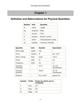
This document is a technical manual published by IDC Technologies that provides formulas and conversions for engineering concepts. It contains 6 chapters that define physical quantities, units of measurement, the SI system of units, general mathematical formulas, engineering concepts and formulas, and a periodic table and resistor color code reference. The manual is intended to immediately provide readers with practical skills to improve productivity in engineering applications. It is accompanied by award-winning documentation and training from IDC Technologies.


![Formulas and Conversions
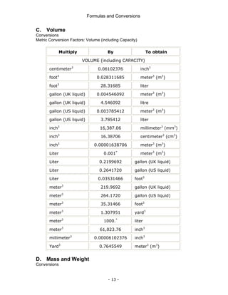
- 39 -
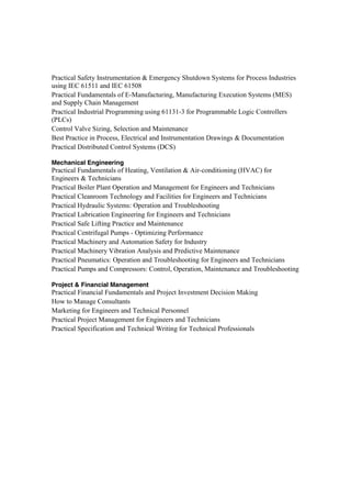
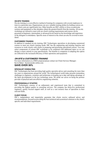
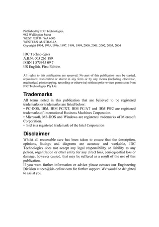
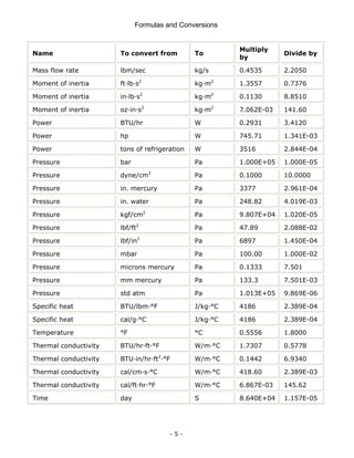
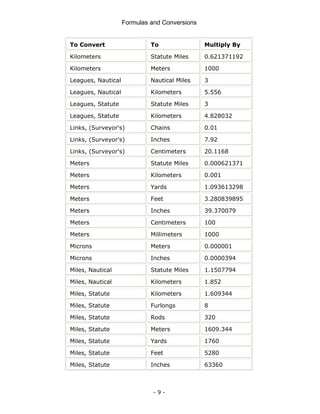
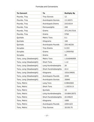
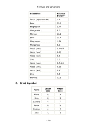
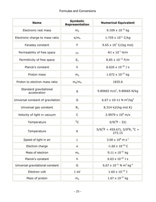
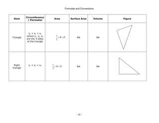
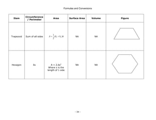
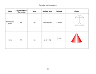
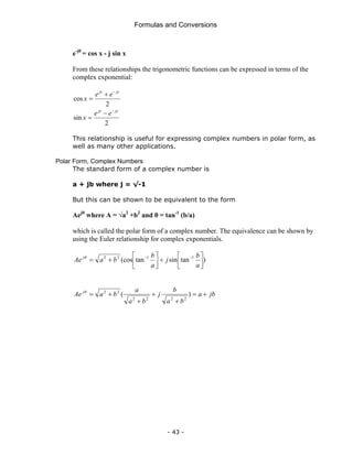
4.3 Trigonometry
A. Pythagoras' Law
c2
= a2
+ b2
B. Basic Ratios
•Sin θ = a/c
•Cos θ = b/c
•Tan θ = a/b
•Cosec θ = c/a
•Sec θ = c/b
•Cot θ = b/a
Degrees versus Radians
•A circle in degree contains 360 degrees
•A circle in radians contains 2π radians
Sine, Cosine and Tangent
sin
opposite
hypotenus
θ = cos
adjacent
hypotenus
θ = tan
opposite
adjacent
θ =
Sine, Cosine and the Pythagorean Triangle
[ ] [ ]
2 2 2 2
sin cos 1
sin cos θ θ
θ θ
+ = + =
c
a
b
θ
θ
opposite
adjacent
hypotenuse](https://image.slidesharecdn.com/frmulaspocketguide-211007091159/85/The-IDC-Engineers-45-320.jpg)
![Formulas and Conversions
- 46 -
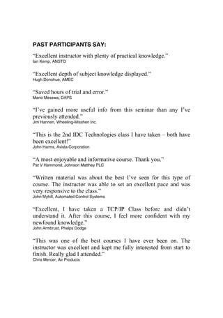
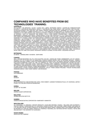
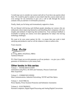
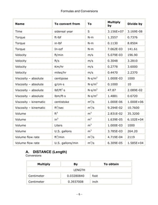
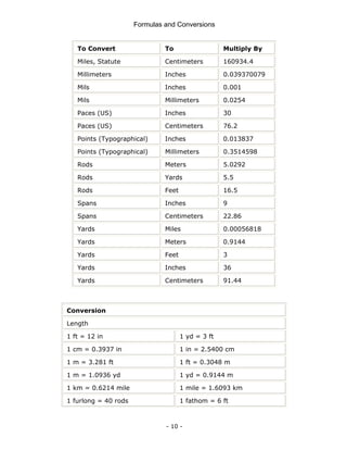
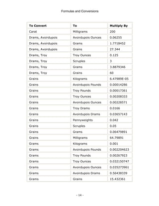
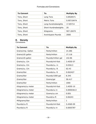
Where EG = generated e.m.f.
EB = generated back e.m.f.
Ia = armature current
Ra = armature resistance
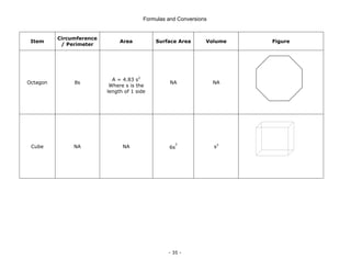
Alternating Current
RMS value of sine curve = 0.707 of maximum value
Mean Value of Sine wave = 0.637 of maximum value
Form factor = RMS value / Mean Value = 1.11
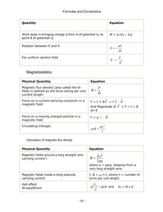
Frequency of Alternator =
60
pN
cycles per second
Where p is number of pairs of poles
N is the rotational speed in r/min
Slip of Induction Motor
[(Slip speed of the field – Speed of the rotor) / Speed of the Field] × 100
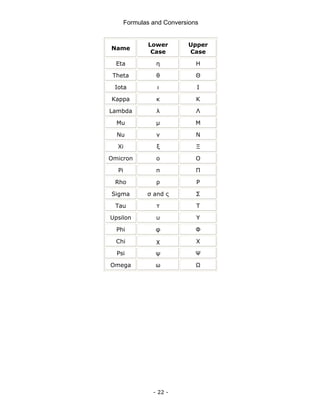
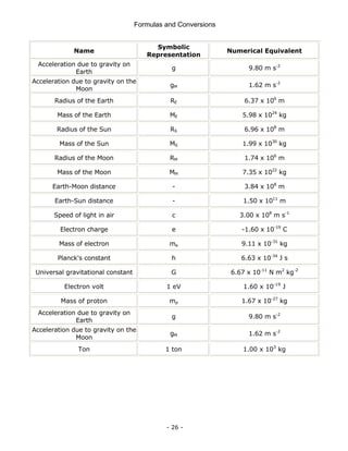
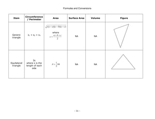
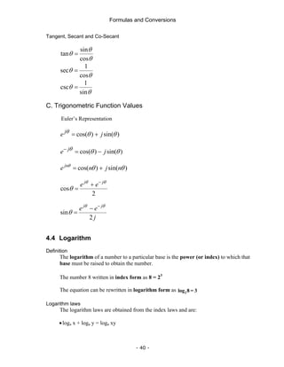
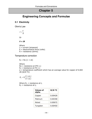
Inductors and Inductive Reactance
Physical Quantity Equation
Inductors and Inductance
VL = L
t
d
i
d
Inductors in Series: LT = L1 + L2 + L3 + . . . .
Inductor in Parallel:
.....
L
1
L
1
L
1
L
1
3
2
1
T
+
+
+
=
Current build up
(switch initially closed after having
been opened)
At τ
t
-
L e
E
t)
(
v =
)
e
-
E(1
t)
(
v
t
R
τ
−
=
τ
t
-
e
1
(
R
E
i(t) −
= )
τ =
R
L
Current decay
(switch moved to a new position)
τ′
=
t
-
o e
I
i(t)
vR(t) = R i(t)
vL(t) = − RT i(t)](https://image.slidesharecdn.com/frmulaspocketguide-211007091159/85/The-IDC-Engineers-52-320.jpg)
![Formulas and Conversions
- 48 -
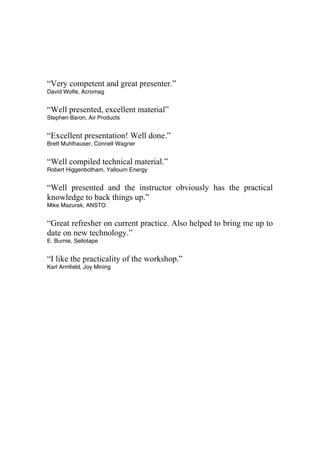
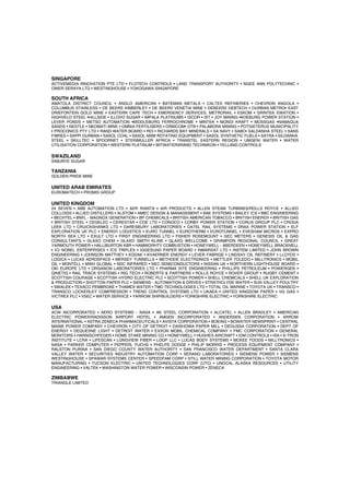
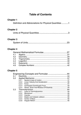
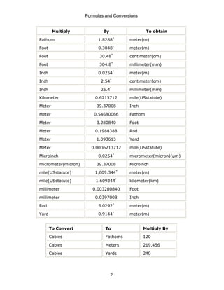
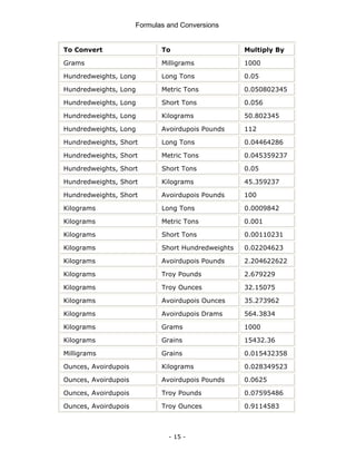
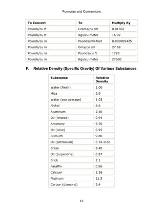
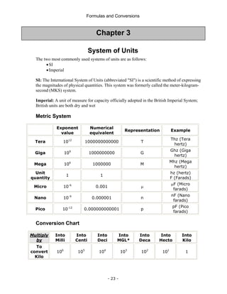
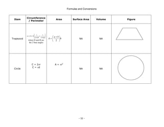
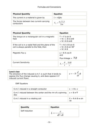
Quantity Equation
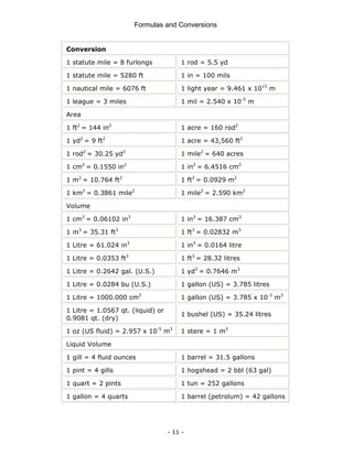
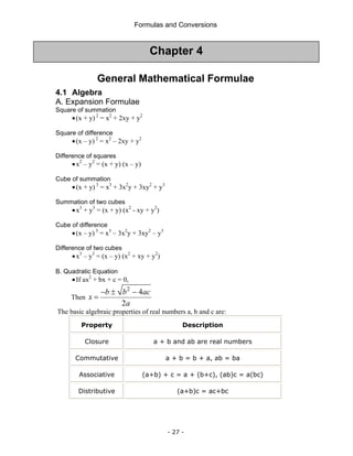
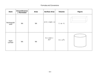
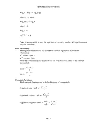
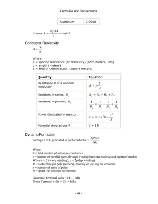
Current Divider Rule
x
T
T
x
Z
Z
I
I =
Two impedance values in
parallel
2
1
2
1
T
Z
Z
Z
Z
Z
+
=
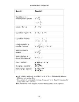
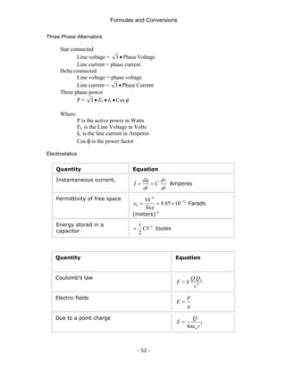
Capacitance
Capacitors
C =
V
Q
[F] (Farads)
Capacitor in Series
.....
C
1
C
1
C
1
C
1
3
2
1
T
+
+
+
=
Capacitors in Parallel .....
C
C
C
C 3
2
1
T +
+
+
=
Charging a Capacitor
RC
t
-
e
R
E
i(t) =
RC
t
-
R e
E
t)
(
v =
)
e
-
E(1
t)
(
v RC
t
-
C =
τ = RC
Discharging a
Capacitor
τ′
−
=
t
-
o
e
R
V
i(t)
τ′
−
=
t
-
o
R e
V
t)
v (
τ′
=
t
-
o
C e
V
t)
v (
τ' = RTC
Quantity Equation
Capacitance
V
Q
C =](https://image.slidesharecdn.com/frmulaspocketguide-211007091159/85/The-IDC-Engineers-54-320.jpg)
![Formulas and Conversions
- 50 -
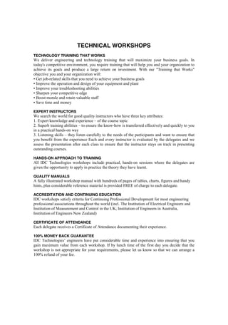
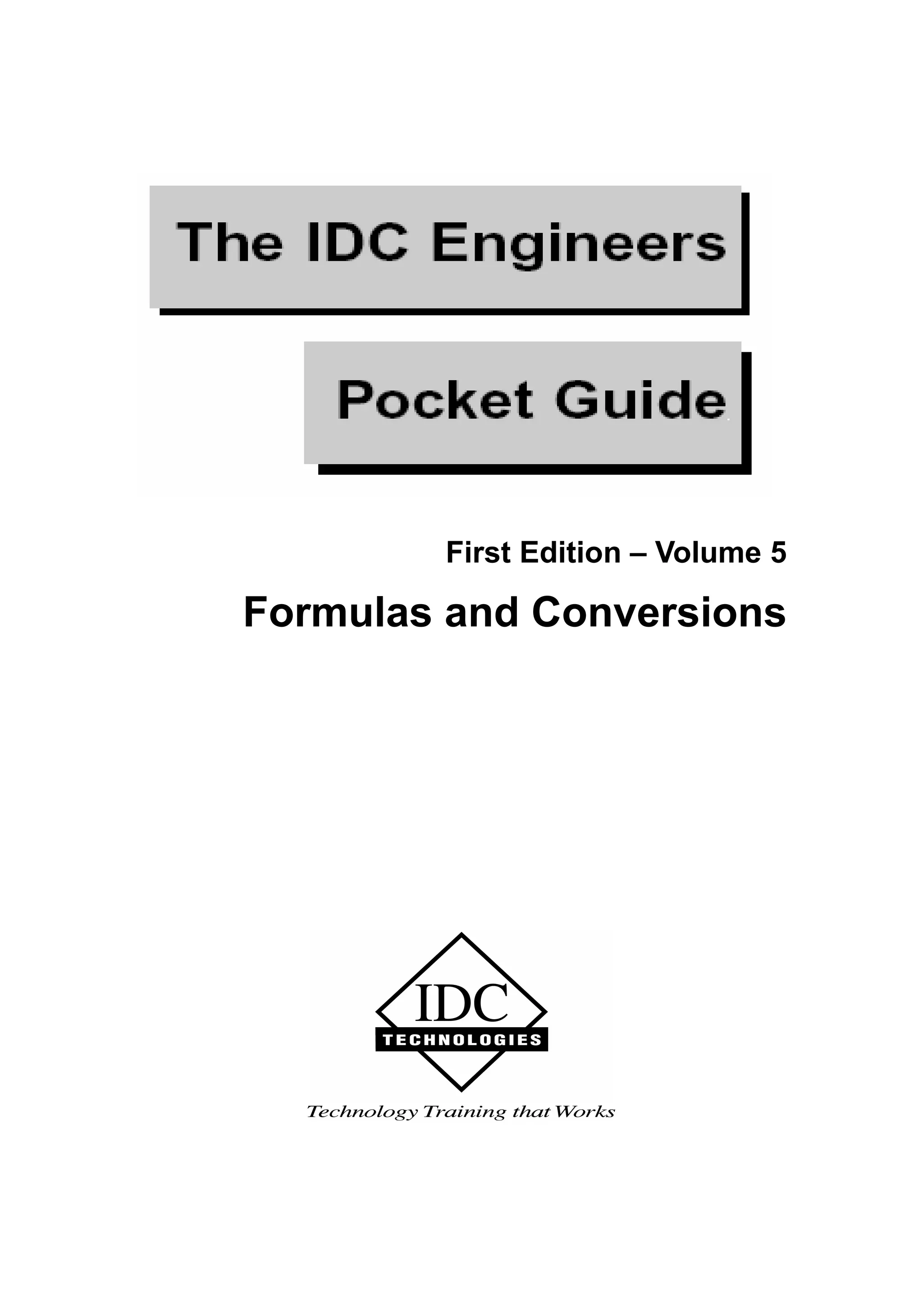
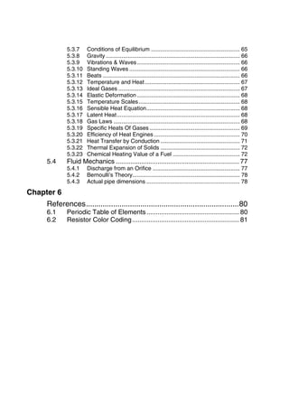
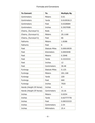
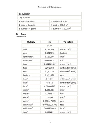
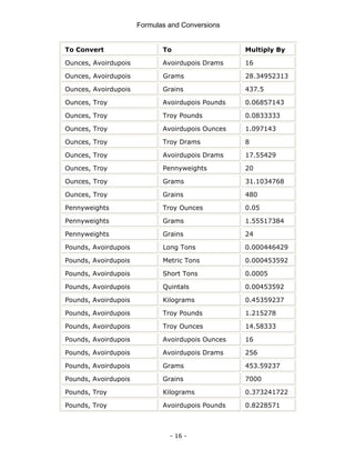
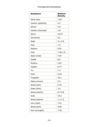
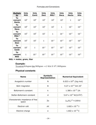
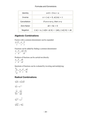
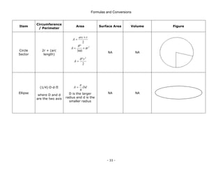
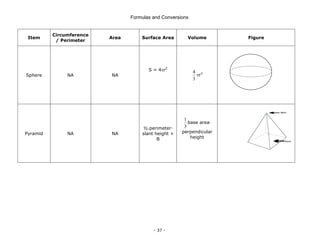
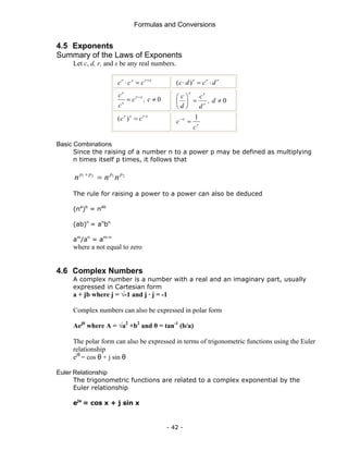
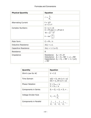
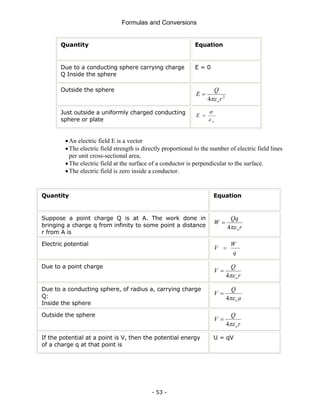
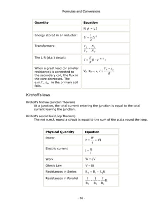
Current in AC Circuit
RMS Current
In Cartesian
form ⎥
⎦
⎤
⎢
⎣
⎡
⎟
⎠
⎞
⎜
⎝
⎛
−
−
⋅
⎥
⎥
⎦
⎤
⎢
⎢
⎣
⎡
⎟
⎠
⎞
⎜
⎝
⎛
−
+
=
C
L
j
R
C
L
R
V
I
ω
ω
ω
ω
1
1
2
2
Amperes
In polar form
s
C
L
R
V
I φ
ω
ω
−
∠
⎟
⎠
⎞
⎜
⎝
⎛
−
+
=
]
1
[
2
2
Amperes
where
⎥
⎥
⎥
⎦
⎤
⎢
⎢
⎢
⎣
⎡
−
= −
R
C
L
s
ω
ω
φ
1
tan 1
Modulus
2
2 1
⎟
⎠
⎞
⎜
⎝
⎛
−
+
=
C
L
R
V
I
ω
ω
Amperes
Complex Impedance
In Cartesian
form ⎟
⎠
⎞
⎜
⎝
⎛
−
+
=
C
L
j
R
Z
ω
ω
1
Ohms
In polar form
s
C
L
R
Z φ
ω
ω ∠
⎟
⎠
⎞
⎜
⎝
⎛
−
+
=
2
2 1
Ohms
Where
⎥
⎥
⎥
⎦
⎤
⎢
⎢
⎢
⎣
⎡
−
= −
R
C
L
s
ω
ω
φ
1
tan 1
Modulus
=
Z
2
2 1
[ ⎟
⎠
⎞
⎜
⎝
⎛
−
+
C
L
R
ω
ω ] Ohms](https://image.slidesharecdn.com/frmulaspocketguide-211007091159/85/The-IDC-Engineers-56-320.jpg)
![Formulas and Conversions
- 61 -
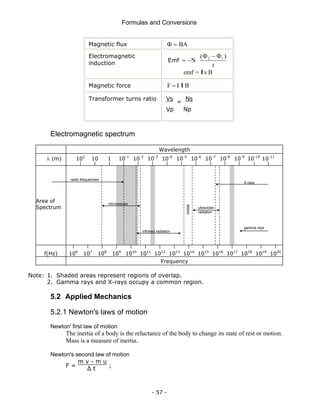
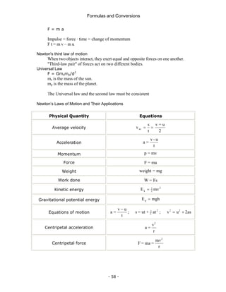
Tangential acceleration aT is due to angular acceleration
α
aT = rα
Centripetal (Centrifugal) acceleration ac is due to change
in direction only
ac = v2
/r = r ω2
Total acceleration, a, of a rotating point experiencing
angular acceleration is the vector sum of aT and ac
a = aT + ac
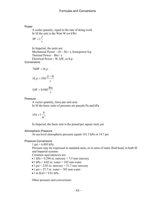
5.2.3 Force
Vector quantity, a push or pull which changes the shape and/or motion of an object
In SI the unit of force is the newton, N, defined as a kg m
In Imperial the unit of force is the pound lb
Conversion: 9.81 N = 2.2 lb
Weight
The gravitational force of attraction between a mass, m, and the mass of the Earth
In SI weight can be calculated from Weight = F = mg, where g = 9.81 m/s2
In Imperial, the mass of an object (rarely used), in slugs, can be calculated from the
known weight in pounds
g
weight
m =
2
2
.
32
s
ft
g =
Torque Equation
T = I α where T is the acceleration torque in Nm, I is the moment of inertia in kg m2
and
α is the angular acceleration in radians/s2
Momentum
Vector quantity, symbol p,
p = mv [Imperial p = (w/g)v, where w is weight]
in SI unit is kgm / s
Work
Scalar quantity, equal to the (vector) product of a force and the displacement of an
object. In simple systems, where W is work, F force and s distance
W = F s
In SI the unit of work is the joule, J, or kilojoule, kJ
1 J = 1 Nm
In Imperial the unit of work is the ft-lb
Energy
Energy is the ability to do work, the units are the same as for work; J, kJ, and ft-lb](https://image.slidesharecdn.com/frmulaspocketguide-211007091159/85/The-IDC-Engineers-67-320.jpg)
![Formulas and Conversions
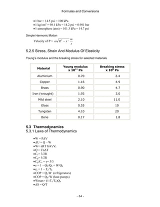
- 66 -
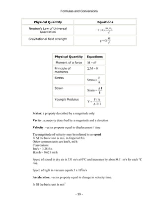
5.3.7 Conditions of Equilibrium
•∑ Fx = 0
•∑ Fy = 0
•∑τ = 0 (any axis)
5.3.8 Gravity
•F = Gm1m2/r2
•T = 2π / √r3
/GMs
•G = 6.67 x 10⁻¹¹
N-m2
/kg2
•g = GME / R2
E
•PE = - Gm1m2 / r
•ve = √2GME / RE
•vs = √GME / r
•ME = 5.97 x 1024
kg
•RE = 6.37 x 10⁶
m
5.3.9 Vibrations & Waves
•F = -kx
•PEs = ½kx2
•x = Acosθ = Acos(ωt)
•v = -Aωsin(ωt)
•a = -Aω2
cos(ωt)
•ω = √k / m
•f = 1 / T
•T = 2π√m / k
•E = ½kA2
•T = 2π√L / g
•vmax = Aω
•amax = Aω2
•v = λ f v = √FT/μ
•μ = m/L
•I = P/A
•β = 10log(I/Io)
•Io = 1 x 10-12
W/m2
•f’
= f[(1 ± v0/v)/(1 μ vs/v)]
•Surface area of the sphere = 4πr2
•Speed of sound waves = 343 m/s
5.3.10 Standing Waves
•fn = nf1
•fn = nv/2L (air column, string fixed both ends) n = 1,2,3,4…….
•fn = nv/4L (open at one end) n = 1,3,5,7………
5.3.11 Beats](https://image.slidesharecdn.com/frmulaspocketguide-211007091159/85/The-IDC-Engineers-72-320.jpg)
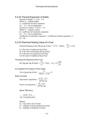
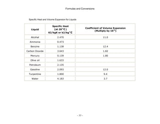
![Formulas and Conversions
- 71 -
[ ]
)
1
(
)
1
(
1
1 1
−
+
−
−
= −
β
γ
β
η γ
γ
k
k
r
k
v
Where rv= cylinder volume / clearance volume
k = absolute pressure at the end of constant V heating (combustion) / absolute pressure at
the beginning of constant V combustion
β = volume at the end of constant P heating (combustion) / clearance
volume
Gas Turbines (Constant Pressure or Brayton Cycle)
⎟
⎟
⎠
⎞
⎜
⎜
⎝
⎛ −
−
=
γ
γ
η 1
1
1
p
r
where rp = pressure ratio = compressor discharge pressure / compressor intake pressure
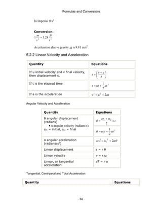
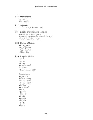
5.3.21 Heat Transfer by Conduction
Material Coefficient of Thermal
Conductivity
W/m °C
Air 0.025
Brass 104
Concrete 0.85
Cork 0.043
Glass 1.0
Iron, cast 70
Steel 60
Wallboard,
paper
0.076
Aluminum 206
Brick 0.6
Copper 380
Felt 0.038
Glass, fibre 0.04
Plastic, cellular 0.04
Wood 0.15](https://image.slidesharecdn.com/frmulaspocketguide-211007091159/85/The-IDC-Engineers-77-320.jpg)