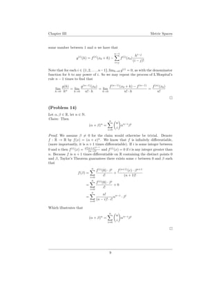
This document contains the proof of several claims regarding differentiation. It begins by proving that the derivative of a function f at a point x0 can be written as the limit of (f(x0 + h) - f(x0 - h))/2h as h approaches 0. It then shows that the derivative is a linear transformation and proves the Cauchy Mean Value Theorem. Finally, it proves some additional results about derivatives and differentiability.

1. Math 441: Chapter V, Differentiation
Leonardo Di Giosia
Problem 2
Let U ⊂ R be open. Let f : U → R be differentiable at some x0 ∈ U.
(a)
Claim:
f (x0) = lim
h→0
f(x0 + h) − f(x0 − h)
2h
Proof. The textbook declares that
f (x0) = lim
h→0
f(x0 + h) − f(x0)
h
(Eq. I)
We now show that
f (x0) = lim
h→0
f(x0) − f(x0 − h)
h
1

2. Chapter III Metric Spaces
By defintion,
f (x0) = lim
x→x0
f(x) − f(x0)
x − x0
Consider the function h(x) = x0 − x. Because h is continuous everywhere,
lim
x→x0
h(x) = h(x0) = 0
So we must have that
f (x0) = lim
x→x0
f(x) − f(x0)
x − x0
= lim
h→0
f(x0 − h) − f(x0)
−h
= lim
h→0
f(x0) − f(x0 − h)
h
(Eq. II)
By combining Equations I and II, we find that
f (x0) = lim
h→0
f(x0 + h) − f(x0 − h)
2h
(b.)
Let α, β ∈ R.
Claim:
lim
h→0
f(x0 + αh) − f(f0 + βh)
h
= (α − β)f (x0)
Proof. We first demonstrate that if η ∈ R,
lim
h→0
f(x0 + ηh) − f(x0)
h
= η · f (x0)
Case I: η = 0, Then the above holds by direct computation.
Case II: η = 0. Denote
γ(h) = x0 + ηh
Then γ is continuous everywhere and because limh→0 γ(h) = x0, we have the
following
lim
h→0
f(x0 + ηh) − f(x0)
h
= lim
γ→x0
f(γ) − f(x0)
h(γ)
= lim
γ→x0
f(γ) − f(x0)
γ−x0
η
= η · f (x0)
2

3. Chapter III Metric Spaces
Hence,
lim
h→0
(f(x0 + αh) − f(f0 + βh)
h
= lim
h→0
f(x0 + αh) − f(x0)
h
+ lim
h→0
f(x0) − f(x0 + βh)
h
= αf (x0) − βf (x0)
= (α − β)f (x0)
So, in both cases, we have the desired result.
(Problem 6)
Let f : R → R be differentiable everywhere with bounded derivative.
Claim: f is uniformly continuous on R.
Proof. Let M > 0 be some upper bound of f (x) on R. Let x0 ∈ R. Denote the
following functions, Ax0
: R → R and Bx0
: R → R by the following
Ax0 (x) = f(x0) + M(x − x0)
Bx0 (x) = f(x0) − M(x − x0)
Let x1 be any point of R greater than x0. If we assume that Ax0 (x1) ≤ f(x1)
we discover that
M ≤
f(x1) − f(x0)
x1 − x0
Which would imply (by Role’s Theorem) that there exists a point c ∈ (x0, x1)
such that M ≤ f (c), which is absurd, so we must have that
x1 > x0 → f(x1) < Ax0 (x1) (Implication I)
Similarly, if we assume Bx0 (x1) ≥ f(x1) we discover there is a point d ∈ (x0, x1)
such that f (d) ≤ −M, which again ilustrates
x1 < x0 → Bx0 (x1) < f(x1) (Implication II)
By paralell reasoning, we may find that
x2 < x0 → Ax0
(x2) < f(x2) < Bx0
(Implication III)
We now use the above information to conclude that f must be uniformly con-
tinuous. Let > 0. Let δ( ) = M . Let x, y ∈ R such that 0 < |x − y| < M .
Without loss of generality, x < y. Denote p = x+y
2 and consider the functions
Ap(x), Bp(x). We know x < p < y, so we utilize Implications I, II, and III. So
we have the following system of inequalities:
Bp(y) <f(y) < Ap(y)
−Bp(x) < −f(x) < −Ap(x)
3

4. Chapter III Metric Spaces
By combining and computing, we find that
M(y − x) < f(y) − f(x) < M(y − x)
So, we see that
|f(y) − f(x)| < M(y − x) < M ·
M
=
So f is uniformly continuous on R.
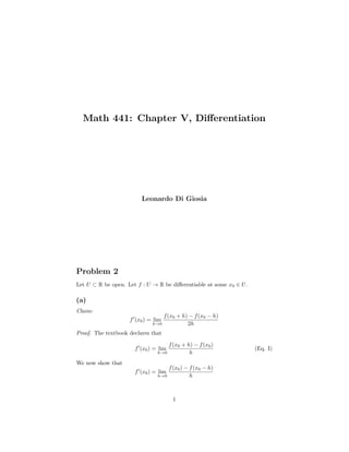
(Problem 7)
Let α, β ∈ R such that α < β. Let U be some open interval in R containing
[α, β]. Let f : U → R be differentiable on R such that f (α) < f (β) and let
γ ∈ R between f (α) and f (β).
Claim: Then there exists some c ∈ (α, β) such that f (c) = γ.
Proof. Consider the set
S = {(x, y) ∈ R2
|α ≤ x < y ≤ β}
Define function g : S ∪ {(α, α), (β, β)} → R by
g(x, y) = f(x)−f(y)
x−y if x = y
g(x, y) = f (x) if x = y
Because f is continuous on [α, β], we know g is continuous on S. We see that g
must also be continuous at the point (α, α) because
lim
(x,y)→(α,α)
f(x) − f(y)
x − y
= f (α)
(The same holds for the point (β, β)). So we see that g is continuous on its
domain. Additionally, wee see that this domain is connected (This may require
a proof, but we skip it here). Because g(α, α) = f (α), g(β, β) = f (β) and
because f (α) < γ < f (β), by the generalized intermediate value theorem
(which extends the domain of real valued continuous functions from intervals in
R to any connected metric space), we must have some point (x0, y0) ∈ S such
that g(x0, y0) = γ. That is, [x0, y0] ⊂ (α, β) such that
f(y0) − f(x0)
y0 − x0
= γ
Finally, because f is differentiable on (x0, y0), we must have some c ∈ (α, β)
such that
f (c) = γ
4

5. Chapter III Metric Spaces
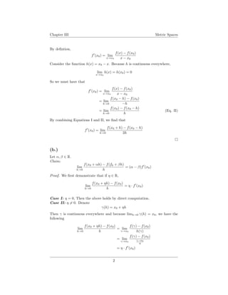
(Problem 8)
Let α, β ∈ R such that α < β and let f, g : [α, β] → R such that f and g are
continuous on [α, β] and differentiable on (α, β)
Claim: Then there exists some c ∈ (α, β) such that f (c)(g(β) − g(α)) =
g (c)(f(β) − f(α)). (The Cauchy Mean Value Theorem).
Proof. Consider the function F : [α, β] → R by
F(x) = (f(x) − f(α))(g(β) − g(α)) − (g(x) − g(α))(f(β) − f(α))
Because a finite product and difference of differentiable functions is differen-
tiable, we must have that F is differentiable on (α, β). Additionally, because
F(α) = F(β) = 0, Rolle’s Theorem guarantees the existence of a c ∈ (α, β) such
that
F (c) = 0
f (c)(g(β) − g(α)) − g (c)(f(β) − f(α) = 0
f (c)(g(β) − g(α)) = g (c)(f(β) − f(α)
(Problem 9)
Let U = be an open interval with extremity a in R and let f and g be differ-
entiable real valued functions on U, with g and g nowhere zero on U. Suppose
that limx→a f(x) = limx→a g(x) = 0. Let limx→a
f (x)
g (x) exist.
(a)
Claim:
lim
x→a
f
g
(x) = lim
x→a
f
g
(x)
(L’Hopsital’s rule)
Proof. (Note that we will assume a is a lower extremity, for notation’s conve-
nience. Result would prove the claim if a were an upper extremity too). Because
a is a lower extremity of U, there exists some 0 > 0 such that if x ∈ R such that
a < x < a+ 0 then x ∈ U. Let be some real number such that a < < a+ 0.
Then f and g are defined and differentiable on (a, a + ). So, by the Cauchy
Mean Value Theorem (Problem 8), we know there exists some c( ) ∈ (a, a + )
such that
f (c( )) · g(a + ) = g (c( )) · f(a + )
(Note: There is a subtlety here. Technically, f and g are not defined at a.
However, their domain of definition may be extended to include a where f(a) =
5

6. Chapter III Metric Spaces
g(a) = 0 while maintaining both continuity of f and g on [a, a + 0) as well as
differentiability on (a, a + 0). In this manner, we have the above result, the
guaranteed existence of c( ), regardless). By hypothesis, g (c( )) and g(a + )
are nonzero. So, for all ∈ (a, a + 0),
f
g
(c( )) =
f
g
(a + )
It is easily demonstrable that c : (a, a + 0) → R is such that lim →0 c( ) = a.
Thus, we have the following:
lim
x→a
f
g
(x) = lim
→0
f(a + )
g(a + )
= lim
→0
f (c( ))
g (c( ))
= lim
x→a
f
g
(x)
(b)
Let f and g be of the above conditions, except limx→a
1
f(x) = 0, limx→a
1
g(x) = 0.
Proof. Because limx→a
1
f(x) is defined, 1
f(x) must be defined/f is non zero on
some subset V ⊂ U with a as an extremity. Define F : V ∪ {a} → R, G :
V ∪ {a} → R by
F(x) = 1
f(x) x ∈ V
G(x) = 1
g(x) x ∈ V
And where F(a) = G(a) = 0. This implies that F, G are continuous at the point
a. Because f is nowhere zero and differentiable on V , we know that F must be
differentiable on all of V . We also know that G is differentiable on all of V . Let
> 0 such that a + ∈ V . Then F, G are continuous on [a, a + ], differentiable
on (a, a + ), and by the Cauchy Mean Value theorem, there must exist some
c( ) such that
F (c( ))G(a + ) = G (c( ))F(a + )
f (c( ))
f2(c( ))g(a + )
=
g (c( ))
g2(c( ))f(a + )
f
g
(c( )) =
f2
(c( ))g(a + )
g2(c( ))f(a + )
The last step is valid due to the fact that g”(c( )) is not zero. Because
6

7. Chapter III Metric Spaces
lim →0 c( ) = lim →0 a + = a, we see that
lim
→0
f
g
(c( )) = lim
→0
f2
(c( ))g(a + )
g2(c( ))f(a + )
lim
x→a
f
g
(x) = lim
x→a
f2
(x)g(x)
g2(x))f(x)
= lim
x→a
f
g
(x)
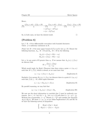
(Problem 10)
Let f, g : R → R be n times differentiable.
Claim: Then f ◦ g is also n times differentiable.
Proof. We proceed by the principle of mathematical induction. In the base case,
f and g are both once differentiable and it is clear from the chain rule presented
in the textbook that at each point x0 ∈ R we have that f ◦ g is differentiable
at x0 so f ◦ g is a differentiable function. So, for some k ≥ 1 we know that any
two real valued functions defined on R which are k times differentiable have a
k times differentiable composition (Induction hypothesis). Let f and g be k + 1
times differentiable functions. Because they are also at least once differentiable,
we know that f ◦ g is once differentiable with derivative given by the chain rule
as
[f ◦ g] = (f ◦ g) · g
Next, we see that because g is k + 1 times differentiable, we know that g is k
times differentiable. Additionally, we have that both f and g are k times dif-
ferentiable, so by the induction hypothesis, f ◦ g is also k times differentiable.
Because the product of two k times differentiable functions is also k times dif-
ferentiable (a fact easily demonstrable with an inductive proof far more simple
than this one), we have that (f ◦ g) · g is also k times differentiable. So [f ◦ g]
is k times differentiable implying that f ◦ g is k + 1 times differentiable, proving
the induction step. Thus, by the principle of mathematical induction, for any
natural number n, if f and g are real valued functions on the real line and are
n times differentiable, then so is their composition.
(Problem 11)
Let f be some real valued function on an open U ⊂ R that is twice differentiable
at x0 ∈ U. Let f (x0) = 0 and f (x0) < 0.
Claim: Then there exists some δ > 0 such that if x ∈ Bδ(x0) then f(x) < f(x0)
Proof. We begin by establishing a brief result. If g : R → R such that
limx→ag(x) = h < 0, then there exists some δ such that |x − a| < δ implies
7

8. Chapter III Metric Spaces
g(x) < 0. Reasoning: Because the limit exists and because −h > 0 we have
some δ such that if |x − a| < δ, then
|g(x) − h| < −h
g(x) − h < −h
g(x) < 0
So the result is proven. We now move on to the rest of the proof. Because f is
differentiable at x0, (AKA, f (x0) exists), there exists some δm such that f is
defined on Bδm (x0). Because f (x0) is negative, by the previous result, there
exists some δn such that if 0 < |x − x0| < δn then
f (x) − f (x0)
x − x0
< 0
f (x)
x − x0
< 0
Denote δp = min{δm, δn}. Assume there exists some y ∈ Bδp
(x0) − {x0} such
that f(y) ≥ f(x0).
Case I: y < x0. Then the quantity f(x0)−f(y)
x0−y is nonpositive and because f
is differentiable on (y, x0), there exists (by the Mean Value Theorem) some
c ∈ (y, x0) such that f (c) ≤ 0, and so f (c)
c−x0
≥ 0. However, by construction,
because c ∈ Bδn
, this quantity f (c)
c−x0
should be negative. So our assumption was
faulty.
Case II: y > x0. Then the quantity f(x0)−f(y)
x0−y is nonnegative and be-
cause f is differentiable on (x0, y), there exists (by the Mean Value Theorem)
some c ∈ (x0, y) such that f (c) ≥ 0, and so f (c)
c−x0
≥ 0. However, by con-
struction, because c ∈ Bδn , this quantity f (c)
c−x0
should be negative. So our
assumption was faulty.
In both cases, it is apparent that our assumption was fallacious, and we must
have that f(y) < f(x0), proving the claim.
(Problem 13)
Let U be an open subset of R and let f : U → R be n times differentiable at
the point x0 ∈ U.
Claim: Then
lim
h→0
f(x0 + h) −
n−1
i=0 f(i)
(x0)hi
i!
hn
=
f(n)
(x0)
n!
Proof. We utilize the previously established L’Hospital’s rule. Observe that the
top left function, which we will denote g(x), is infinitely differentiable. If j is
8

9. Chapter III Metric Spaces
some number between 1 and n we have that
g(i)
(h) = f(i)
(x0 + h) −
n−1
i=j
f(i)
(x0)
hi−j
(i − j)!
Note that for each i ∈ {1, 2, . . . , n−1}, limh→0 g(i)
= 0, as with the denominator
function for h to any power of i. So we may repeat the process of L’Hospital’s
rule n − 1 times to find that
lim
h→0
g(h)
hn
= lim
h→0
g(n−1)
(x0)
n! · h
= lim
h→0
f(n−1)
(x0 + h) − f(n−1)
n! · h
=
f(n)
(x0)
n!
(Problem 14)
Let α, β ∈ R, let n ∈ N.
Claim: Then
(α + β)n
=
n
i=0
n
i
αn−i
βi
Proof. We assume β = 0 for the claim would otherwise be trivial. Denote
f : R → R by f(x) = (α + x)n
. We know that f is infinitely differentiable,
(more importantly, it is n + 1 times differentiable). If i is some integer between
0 and n then f(i)
(x) = n!(α+x)n−i
(n−i)! and f(i)
(x) = 0 if i is any integer greater than
n. Because f is n + 1 times differentiable on R containing the distinct points 0
and β, Taylor’s Theorem guarantees there exists some c between 0 and β such
that
f(β) =
n
i=0
f(i)
(0) · βi
i!
+
f(n+1)
(c) · βn+1
(n + 1)!
=
n
i=0
f(i)
(0) · βi
i!
+ 0
=
n
i=0
n!
(n − i)! · i!
αn−i
· βi
Which illustrates that
(α + β)n
=
n
i=0
n
i
αn−i
βi
9

10. Chapter III Metric Spaces
(Problem 15)
Let f be a continuous real valued function on the closed interval of extremities
a and b which is (n + 1) times differentiable on the open interval with the same
extremities. Suppose that limx→a f(i)
(x) exists and that f(i)
is bounded for
i ∈ {1, 2, . . . , n}.
Claim: Then there exists some c between a and b such that
f(b) = f(a) +
n
i=1
lim
x→a
f(i)
(x)
(b − a)i
i!
+ f(n+1)
(c)
(b − a)n+1
(n + 1)!
(Strong Taylor’s Theorem)
Proof. Define Rn(b, a) by
f(b) = f(a) +
n
i=1
lim
x→a
f(i)
(x)
(b − a)i
i!
+ Rn(b, a)
If x is any element of the interval, we define Rn(b, x) with
f(b) = f(x) +
n
i=0
f(i)
(x)
(b − x)i
i!
+ Rn(b, x)
In the above, we see that because the left side is differentiable, f(x) is differ-
entiable as well as the sum is differentiable on the interval, we must have that
Rn(b, x) is a differentiable function (with respect to x) on the interval. Explicitly
computing the derivative shows that
d
dx
Rn(b, x) = −
f(n+1)
(x)(b − x)n
n!
(For an explicit explanation of this derivation process, see the textbook’s work
in proving the weaker version of Taylor’s Theorem). Because a = b, we know
that there must exist some real number K such that
Rn(b, a) = K
(b − a)n+1
(n + 1)!
(Note that this is simply a result of the Archimedean principle). Define the
real valued function Ψ on the closed interval by Ψ(x) = Rn(b, x) − K (b−x)n+1
(n+1)! .
We want to be able to apply Rolle’s theorem to this function on our interval,
requiring differentiability on the open and continuity on the closed. We know
that because Rn(b, x) is differentiable on the open interval, so is Ψ, proving
that Ψ is continuous on the open interval. Now, we just need to show that Ψ is
continuous at the extremities a and b (note that this is the bit which separates
10

11. Chapter III Metric Spaces
the weak from the strong version of Taylor’s Theorem).
lim
x→a
Ψ(x) = lim
x→a
f(b) − f(x) −
n
i=1
f(i) (b − x)i
i!
+ K
(b − x)n+1
(n + 1)!
= f(b) − f(a) −
n
i=1
lim
x→a
f(i)
(x)
(b − a)i
i!
+ K
(b − a)n+1
(n + 1)!
= Rn(b, a) + K
(b − a)n+1
(n + 1)!
= Ψ(a)
So Ψ is continuous at a. We consider limx→b Ψ(x).
lim
x→b
Ψ(x) = lim
x→b
f(b) − f(x) −
n
i=1
f(i) (b − x)i
i!
+ K
(b − x)n+1
(n + 1)!
= −
n
i=1
lim
x→b
f(i)
(x)
(b − x)i
i!
+ 0
But because all derivatives of f are bounded, for any i ∈ {i, 2, . . . , n},
limx→b f(i)
(x) · (b−x)i
i! = 0. Thus.
= 0
= Ψ(b)
Hence, Ψ is continuous at b. Because Ψ(a) = Ψ(b) = 0, there must exists some
c between a and b (by Rolle’s Theorem) such that
0 = Ψ (c)
=
d
dx
Rn(b, c) + K
(b − c)n
n!
= −f(n+1)
(c)
(b − c)n
n!
+ K
(b − c)n
n!
So, we find that f(n+1)
(c) = K, so Rn(b, a) = f(n+1)
(c)(b−a)n+1
(n+1)! and in total,
there exists some c between a and b such that
f(b) = f(a) +
n
i=1
lim
x→a
f(i)
(x)
(b − a)i
i!
+ f(n+1)
(c)
(b − a)n+1
(n + 1)!
11