This document provides solutions to problems from Chapter 2 and Chapter 3 of the book "Partial Differential Equations" by Lawrence C. Evans. The solutions include:
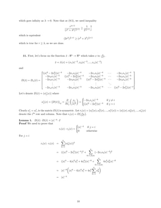
1) Finding an explicit formula for a function satisfying a given PDE.
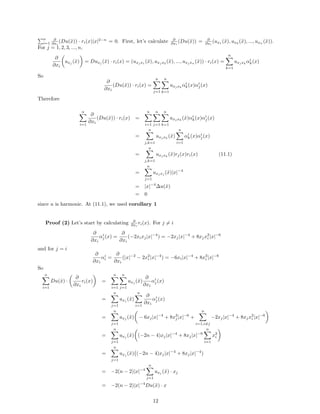
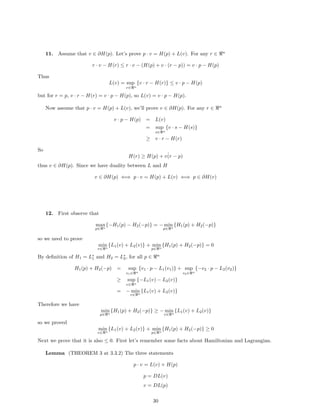
2) Showing that the Laplacian of a transformed function equals the Laplacian of the original function.
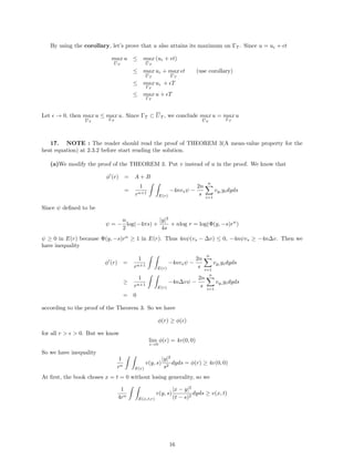
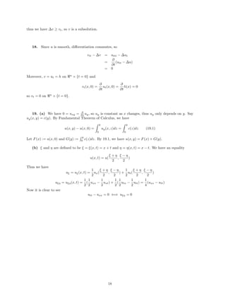
3) Modifying the mean value property for harmonic functions to account for functions satisfying -Δu = f.
This document presents two theorems that solve new types of nonlinear discrete inequalities involving the maximum of an unknown function over a past time interval. These inequalities are discrete generalizations of Bihari's inequality and can be used to study qualitative properties of solutions to nonlinear difference equations with maxima. Theorem 1 provides an upper bound for the solution in terms of inverse functions, while Theorem 2 uses a simpler integral function but a more complicated upper bound. The inequalities are applied to obtain bounds on solutions to difference equations with maxima.
The Solovay-Kitaev Theorem guarantees that for any single-qubit gate U and precision ε > 0, it is possible to approximate U to within ε using Θ(logc(1/ε)) gates from a fixed finite universal set of quantum gates. The proof involves first using a "shrinking lemma" to show that any gate in an ε-net can be approximated to within Cε using a constant number of applications of gates from the universal set. This is then iterated to construct an approximation of the desired gate U to arbitrary precision using a number of gates that scales as the logarithm of 1/ε.
The document discusses series solutions to second order linear differential equations near ordinary points. It provides an example of finding the series solution to the differential equation y'' + y = 0 near x0 = 0. The solution is found to be a cosine series which represents the cosine function, a fundamental solution. A second example finds the series solution to Airy's equation near x0 = 0, obtaining fundamental solutions related to Airy functions.
11.0003www.iiste.org call for paper.common fixed point theorem for compatible...Alexander Decker
This document presents a common fixed point theorem involving six self-mappings of a complete metric space that satisfy certain contractive conditions and compatibility properties. The theorem is proved over multiple steps: 1) a Cauchy sequence is constructed from the mappings and shown to converge, 2) the limit is shown to be a common fixed point using compatibility, and 3) uniqueness of the fixed point is proved using the contractive conditions. The theorem generalizes several existing common fixed point results in the literature involving compatible mappings.
3.common fixed point theorem for compatible mapping of type a -21-24Alexander Decker
This document presents a common fixed point theorem involving six self-mappings of a complete metric space that satisfy certain contractive conditions and compatibility properties. The theorem is proved over multiple steps: 1) a Cauchy sequence is constructed from the mappings and shown to converge to a point z, 2) z is shown to be a common fixed point of the mappings, 3) uniqueness of the common fixed point is proved using the contractive conditions. The theorem generalizes several existing common fixed point results.
1. The document presents a new approach to proving comparison theorems for stochastic differential equations (SDEs) using differentiation of solutions with respect to initial data.
2. It proves that if the drift term of one SDE is always greater than or equal to the other, and their initial values satisfy the same relation, then the solutions will also satisfy this relation for all time.
3. Two methods are provided: the first uses explicit solutions, the second avoids this by showing the difference process cannot reach zero in finite time based on its behavior.
Continuity of functions by graph (exercises with detailed solutions)Tarun Gehlot
The document contains 11 exercises analyzing the continuity of various functions. It begins by verifying the continuity of square root and rational functions at specific points. Later exercises involve determining the domains of piecewise functions and studying their continuity by analyzing limits. Graphs are drawn to illustrate discontinuity points for functions involving floor, trigonometric, and fractional expressions. The solutions find appropriate definitions or parameters to extend functions to continuous forms at boundaries between pieces.
Math 1102-ch-3-lecture note Fourier Series.pdfhabtamu292245
1. The document discusses Fourier series and orthogonal functions. It defines orthogonal functions and provides examples of orthogonal function sets, such as cosine and sine functions.
2. The chief advantage of orthogonal functions is that they allow functions to be represented as generalized Fourier series expansions. The orthogonality of the functions helps determine the Fourier coefficients in a simple way using integrals.
3. Euler's formulae give the expressions for calculating the Fourier coefficients a0, an, and bn of a periodic function f(x) from its values over one period using integrals of f(x) multiplied by cosine and sine terms.
This document summarizes some statistical models used for calibrating imperfect mathematical models. It discusses three main approaches:
1. Gaussian stochastic process (GaSP) calibration, which models bias as a Gaussian process. This is commonly used but can produce inconsistent parameter estimates.
2. L2 calibration, which estimates reality separately from the model before estimating parameters. However, it does not use model information.
3. Scaled Gaussian stochastic process (S-GaSP) calibration, which constrains the GaSP to have a fixed L2 norm. This satisfies predicting reality and calibrated parameters. The S-GaSP is equivalent to penalized kernel ridge regression.
The document analyzes the nonparametric regression setting
This document defines continuity and uniform continuity of functions. A function f is continuous on a set S if small changes in the input x result in small changes in the output f(x). A function is uniformly continuous if the same relationship holds for all inputs and outputs simultaneously, not just for a fixed input. Several examples are provided to illustrate the difference. The key difference is that a continuous function may depend on the specific input point, while a uniformly continuous function does not. Functions that satisfy a Lipschitz inequality are proven to be uniformly continuous.
This lecture discusses dimensionality reduction techniques for big data, specifically the Johnson-Lindenstrauss lemma. It introduces linear sketching as a dimensionality reduction method from n dimensions to t dimensions (where t is logarithmic in n). It then proves the JL lemma, which shows that for t proportional to 1/ε^2, the l2 distances between points are preserved to within a 1±ε factor. As an application, it discusses locality sensitive hashing (LSH) for approximate nearest neighbor search, where points close in distance hash to the same bucket with high probability.
This document discusses various topics related to integration including indefinite and definite integrals, power rules, properties of integrals, integration by parts, u-substitution, and definitions. Some key points covered are:
- Integration was developed independently by Newton and Leibniz in the late 17th century.
- The indefinite integral finds an antiderivative, while the definite integral evaluates the area under a function between bounds.
- Common integration techniques include power rules, integration by parts, and u-substitution.
- Integration rules and properties allow integrals to be transformed and simplified.
This document discusses series solutions near regular singular points of differential equations. It begins by deriving the recurrence relation for the series coefficients from substituting a power series solution into the differential equation. It then shows how to obtain the indicial equation and exponents at the singular point. Two series solutions are given corresponding to the two exponents. An example problem finds the singular points, exponents, and series solutions for a given third order differential equation.
The document discusses Fourier series and their applications. It begins by introducing how Fourier originally developed the technique to study heat transfer and how it can represent periodic functions as an infinite series of sine and cosine terms. It then provides the definition and examples of Fourier series representations. The key points are that Fourier series decompose a function into sinusoidal basis functions with coefficients determined by integrating the function against each basis function. The series may converge to the original function under certain conditions.
This paper presents a generalization of the famous Osgood uniqueness condition for nonlinear Volterra integral equations. Specifically, it considers equations of the form u(x) = ∫_0^x (x-s)^a-1 g(u(s))ds, where a ≥ 1 and g satisfies certain conditions. The paper proves that the trivial solution u(x) = 0 is unique if and only if ∫_0^s φ(t)dt = ∞, where φ is defined in terms of g. This generalizes the classical Osgood condition to allow for nonlinearities g that do not necessarily increase, which has applications in areas like nonlinear diffusion. The proof uses estimates of nontri
This document provides solutions to problems regarding disturbance rejection and integral control. It summarizes the disturbance models for different types of disturbances, including piecewise exponential, piecewise constant, and piecewise harmonic oscillations. It then designs state feedback and feedforward gains to reject disturbances. Finally, it derives the transfer function from disturbance to output and adds integral feedback to reject constant disturbances.
Some Common Fixed Point Theorems for Multivalued Mappings in Two Metric SpacesIJMER
In this paper we prove some common fixed point theorems for multivalued mappings in two
complete metric spaces.
AMS Mathematics Subject Classification: 47H10, 54H25
This document discusses orthogonal functions and polynomial solutions to three specific second order differential equations: the Legendre, Laguerre, and Hermite equations. It shows that polynomial solutions to these equations are orthogonal using Sturm-Liouville theory. This allows functions to be written as Fourier series with respect to the orthogonal polynomial solutions. The Legendre, Laguerre, and Hermite polynomials are explicitly derived and shown to be orthogonal with respect to certain weight functions on their domains.
The document discusses finite speed approximations to the Navier-Stokes equations. It introduces relaxation approximations and a damped wave equation approximation as two methods to derive finite speed approximations. It then discusses a vector BGK approximation, which takes a kinetic approach using a system of hyperbolic equations that approximates the Boltzmann equation and can be shown to converge to the incompressible Navier-Stokes equations in the diffusive limit. The document provides details on the vector BGK model, including compatibility conditions, conservation laws, and proofs of consistency, stability, and existence of global solutions.
This document summarizes research on Ambrosetti-Prodi type results for fully nonlinear fourth order differential equations. It presents methods and techniques used, including:
1) Defining lower and upper solutions to establish existence and location results for solutions.
2) Using a Nagumo-type growth condition and topological degree arguments to prove existence of at least one solution.
3) Establishing a priori bounds on solutions that do not depend on boundary conditions.
It also presents results on the existence and non-existence of solutions depending on a parameter s, and a multiplicity result using strict lower and upper solutions when the topological degree is ±1.
This academic article presents a unique common fixed point theorem for four maps under contractive conditions in cone metric spaces. The authors prove the existence of coincidence points and a common fixed point theorem for four self-maps on a cone metric space that satisfy a contractive condition. They show that if one of the subspaces is complete, then the maps have a coincidence point, and if the maps are commuting, they have a unique common fixed point. This generalizes and improves on previous comparable results in the literature.
This document summarizes a presentation on random entire functions. It discusses three classical families of random entire functions - Gaussian, Rademacher, and Steinhaus entire functions. It presents several theorems regarding inequalities concerning the maximum modulus and zeros of random entire functions. Specifically, it shows that the weighted zero counting function of random entire functions in family Y is close to the logarithm of the maximum modulus function, with an error term that is independent of the probability space. It also establishes an analogy of Nevanlinna's second main theorem for random entire functions in family Y.
The document summarizes the brachistochrone problem from calculus of variations. It introduces the brachistochrone curve as the curve of fastest descent under gravity between two points. The problem is then solved using tools from calculus of variations, arriving at the Euler-Lagrange equation. This equation shows that the brachistochrone curve between two points is a cycloid. Additionally, the document discusses that the cycloid is a tautochronic curve, meaning an object will take the same amount of time to slide from any point on it to the lowest point.
Unique fixed point theorems for generalized weakly contractive condition in o...Alexander Decker
This document summarizes a research paper that proves some new fixed point theorems for generalized weakly contractive mappings in ordered partial metric spaces. The paper extends previous theorems proved by Nashine and Altun in 2017. It presents definitions of partial metric spaces and properties. It proves a new fixed point theorem (Theorem 2.1) for nondecreasing mappings on ordered partial metric spaces that satisfy a generalized contractive condition. The theorem shows the mapping has a fixed point and the partial metric of the fixed point to itself is 0. It uses properties of partial metrics, contractive conditions and continuity to prove the sequence generated by iterating the mapping is Cauchy and converges.
The document discusses quantum mechanical concepts including:
1) The time derivative of the momentum expectation value satisfies an equation involving the potential gradient.
2) For an infinite potential well, the kinetic energy expectation value is proportional to n^2/a^2 and the potential energy expectation value vanishes.
3) Eigenfunctions of an eigenvalue problem under certain boundary conditions correspond to positive eigenvalues that are sums of squares of integer multiples of pi.
(α ψ)- Construction with q- function for coupled fixed pointAlexander Decker
This document presents a theorem to prove the existence of coupled fixed points for contractive mappings in partially ordered quasi-metric spaces. It begins with definitions of key concepts such as mixed monotone mappings, coupled fixed points, quasi-metric spaces, and Q-functions. It then states and proves a coupled fixed point theorem for mappings that satisfy an (α-Ψ)-contractive condition in a partially ordered, complete quasi-metric space with a Q-function. The theorem shows that if such a mapping F has the mixed monotone property and satisfies the contractive inequality, then F has at least one coupled fixed point.
বাংলাদেশের অর্থনৈতিক সমীক্ষা ২০২৪ [Bangladesh Economic Review 2024 Bangla.pdf] কম্পিউটার , ট্যাব ও স্মার্ট ফোন ভার্সন সহ সম্পূর্ণ বাংলা ই-বুক বা pdf বই " সুচিপত্র ...বুকমার্ক মেনু 🔖 ও হাইপার লিংক মেনু 📝👆 যুক্ত ..
আমাদের সবার জন্য খুব খুব গুরুত্বপূর্ণ একটি বই ..বিসিএস, ব্যাংক, ইউনিভার্সিটি ভর্তি ও যে কোন প্রতিযোগিতা মূলক পরীক্ষার জন্য এর খুব ইম্পরট্যান্ট একটি বিষয় ...তাছাড়া বাংলাদেশের সাম্প্রতিক যে কোন ডাটা বা তথ্য এই বইতে পাবেন ...
তাই একজন নাগরিক হিসাবে এই তথ্য গুলো আপনার জানা প্রয়োজন ...।
বিসিএস ও ব্যাংক এর লিখিত পরীক্ষা ...+এছাড়া মাধ্যমিক ও উচ্চমাধ্যমিকের স্টুডেন্টদের জন্য অনেক কাজে আসবে ...
How to Make a Field Mandatory in Odoo 17Celine George
In Odoo, making a field required can be done through both Python code and XML views. When you set the required attribute to True in Python code, it makes the field required across all views where it's used. Conversely, when you set the required attribute in XML views, it makes the field required only in the context of that particular view.
Strategies for Effective Upskilling is a presentation by Chinwendu Peace in a Your Skill Boost Masterclass organisation by the Excellence Foundation for South Sudan on 08th and 09th June 2024 from 1 PM to 3 PM on each day.
This slide is special for master students (MIBS & MIFB) in UUM. Also useful for readers who are interested in the topic of contemporary Islamic banking.
How to Fix the Import Error in the Odoo 17Celine George
An import error occurs when a program fails to import a module or library, disrupting its execution. In languages like Python, this issue arises when the specified module cannot be found or accessed, hindering the program's functionality. Resolving import errors is crucial for maintaining smooth software operation and uninterrupted development processes.
A workshop hosted by the South African Journal of Science aimed at postgraduate students and early career researchers with little or no experience in writing and publishing journal articles.
LAND USE LAND COVER AND NDVI OF MIRZAPUR DISTRICT, UPRAHUL
This Dissertation explores the particular circumstances of Mirzapur, a region located in the
core of India. Mirzapur, with its varied terrains and abundant biodiversity, offers an optimal
environment for investigating the changes in vegetation cover dynamics. Our study utilizes
advanced technologies such as GIS (Geographic Information Systems) and Remote sensing to
analyze the transformations that have taken place over the course of a decade.
The complex relationship between human activities and the environment has been the focus
of extensive research and worry. As the global community grapples with swift urbanization,
population expansion, and economic progress, the effects on natural ecosystems are becoming
more evident. A crucial element of this impact is the alteration of vegetation cover, which plays a
significant role in maintaining the ecological equilibrium of our planet.Land serves as the foundation for all human activities and provides the necessary materials for
these activities. As the most crucial natural resource, its utilization by humans results in different
'Land uses,' which are determined by both human activities and the physical characteristics of the
land.
The utilization of land is impacted by human needs and environmental factors. In countries
like India, rapid population growth and the emphasis on extensive resource exploitation can lead
to significant land degradation, adversely affecting the region's land cover.
Therefore, human intervention has significantly influenced land use patterns over many
centuries, evolving its structure over time and space. In the present era, these changes have
accelerated due to factors such as agriculture and urbanization. Information regarding land use and
cover is essential for various planning and management tasks related to the Earth's surface,
providing crucial environmental data for scientific, resource management, policy purposes, and
diverse human activities.
Accurate understanding of land use and cover is imperative for the development planning
of any area. Consequently, a wide range of professionals, including earth system scientists, land
and water managers, and urban planners, are interested in obtaining data on land use and cover
changes, conversion trends, and other related patterns. The spatial dimensions of land use and
cover support policymakers and scientists in making well-informed decisions, as alterations in
these patterns indicate shifts in economic and social conditions. Monitoring such changes with the
help of Advanced technologies like Remote Sensing and Geographic Information Systems is
crucial for coordinated efforts across different administrative levels. Advanced technologies like
Remote Sensing and Geographic Information Systems
9
Changes in vegetation cover refer to variations in the distribution, composition, and overall
structure of plant communities across different temporal and spatial scales. These changes can
occur natural.
Walmart Business+ and Spark Good for Nonprofits.pdfTechSoup
"Learn about all the ways Walmart supports nonprofit organizations.
You will hear from Liz Willett, the Head of Nonprofits, and hear about what Walmart is doing to help nonprofits, including Walmart Business and Spark Good. Walmart Business+ is a new offer for nonprofits that offers discounts and also streamlines nonprofits order and expense tracking, saving time and money.
The webinar may also give some examples on how nonprofits can best leverage Walmart Business+.
The event will cover the following::
Walmart Business + (https://business.walmart.com/plus) is a new shopping experience for nonprofits, schools, and local business customers that connects an exclusive online shopping experience to stores. Benefits include free delivery and shipping, a 'Spend Analytics” feature, special discounts, deals and tax-exempt shopping.
Special TechSoup offer for a free 180 days membership, and up to $150 in discounts on eligible orders.
Spark Good (walmart.com/sparkgood) is a charitable platform that enables nonprofits to receive donations directly from customers and associates.
Answers about how you can do more with Walmart!"
it describes the bony anatomy including the femoral head , acetabulum, labrum . also discusses the capsule , ligaments . muscle that act on the hip joint and the range of motion are outlined. factors affecting hip joint stability and weight transmission through the joint are summarized.
How to Manage Your Lost Opportunities in Odoo 17 CRMCeline George
Odoo 17 CRM allows us to track why we lose sales opportunities with "Lost Reasons." This helps analyze our sales process and identify areas for improvement. Here's how to configure lost reasons in Odoo 17 CRM
How to Setup Warehouse & Location in Odoo 17 InventoryCeline George
In this slide, we'll explore how to set up warehouses and locations in Odoo 17 Inventory. This will help us manage our stock effectively, track inventory levels, and streamline warehouse operations.
How to Setup Warehouse & Location in Odoo 17 Inventory
evans_pde_solutions_ch2_ch3.pdf
1. Evans PDE Solutions for Ch2 and Ch3
Osman Akar
July 2016
This document is written for the book ”Partial Differential Equations” by Lawrence C. Evans (Second
Edition). The document prepared under UCLA 2016 Pure REU Program.
SOLUTIONS OF CHAPTER 2
1. Consider the function z : < → < for fixed x ∈ <n
and t ∈ (0, ∞)
z(s) = u(x + bs, t + s)ecs
Then
ż(s) :=
∂z
∂s
= ecs
(b · Dxu(x + sb, t + s) + ut(x + sb, t + s) + cu(x + sb, t + s)) = 0
by the condition given by the problem. Therefore, z is a constant function with respect to s. Finally, by
using the fact that u = g on <n
× {t = 0}, we conclude that
u(x, t) = z(0) = z(−t) = u(x − tb, 0)e−ct
= g(x − tb)e−ct
2. Let O = (aij) and φ(x) = O · x. Then it’s clear that Dφ(x) = O. Since v is defined to be
v(x) = u(O · x) = (u ◦ φ)(x), we calculate
Dv(x) = Du(φ(x)) · Dφ(x) = Du(O · x) · O
Then vxi
(x) =
Pn
j=1 uxj
(φ(x))aji. Note that by the same calculations, we have
D(uxj ◦ φ)(x) = Duxj (φ(x)) · O
Therefore
vxixi
(x) =
∂
∂xi
vxi
(x) =
n
X
j=1
∂
∂xi
uxj
(φ(x))aji =
n
X
j=1
aji(
n
X
k=1
uxj xk
(φ(x))aki) =
n
X
j,k=1
ajiakiuxj xk
(φ(x))
The laplacian of v is
∆v(x) =
n
X
i=1
vxixi
(x) =
n
X
i=1
(
n
X
j,k=1
ajiakiuxj xk
(φ(x))) =
n
X
j,k=1
(uxj xk
(φ(x))
n
X
i=1
ajiaki)
Since O is an orthogonal matrix,
n
X
i=1
ajiaki =
(
1 if j = k
0otherwise
Lastly, we conclude our proof with
∆v(x) =
n
X
j=1
(uxj xj
(φ(x)) = ∆u(φ(x)) = 0
1
2. since u is harmonic.
3. We’ll modify the mean value property for harmonic functions. It is assumed that the reader know
the proof of the mean value property(Check Evans PDE 2.2.2, Mean Value Formulas). As in the proof
in the book, define
φ(s) =
1
nα(n)sn−1
Z
∂B(0,s)
u(y)dS(y)
Then the book proves
φ0
(s) =
1
nα(n)sn−1
Z
B(0,s)
∆u(y)dy
Since ∆u = −f in B(0, r)
φ0
(s) =
−1
nα(n)sn−1
Z
B(0,s)
f(y)dy
By Fundamental Theorem of Calculus,
φ(r) − φ() =
Z r
φ0
(s)ds
for any 0. Note that
lim
→0
φ() = lim
→0
1
nα(n)n−1
Z
∂B(0,)
u(y)dS(y)
=
1
m(∂B(0, ))
Z
∂B(0,)
u(y)dS(y)
= u(0) (3.1)
Let’s calculate
R r
φ0
(s)ds
Z r
φ0
(s)ds =
Z r
−1
nα(n)sn−1
Z
B(0,s)
f(y)dyds
=
−1
nα(n)
Z
B(0,r)
f(y)
Z r
max(|y|,)
1
sn−1
dsdy
In the last equality, we changed the order of integration. Note that
Z r
ζ
1
sn−1
ds =
−1
(n − 2)sn−2
3.
4.
5.
6.
7. s=r
ζ
=
1
n − 2
(
1
ζn−2
−
1
rn−2
) (3.2)
Therefore
Z r
φ0
(s)ds =
1
nα(n)
Z
B(0,r)
f(y)
Z r
max(|y|,)
1
sn−1
dsdy
=
−1
nα(n)
(
Z
B(0,r)−B(0,)
f(y)
Z r
|y|
1
sn−1
dsdy +
Z
B(0,)
f(y)
Z r
1
sn−1
dsdy)
=
−1
nα(n)
(
Z
B(0,r)−B(0,)
f(y)
1
n − 2
(
1
|y|n−2
−
1
rn−2
)dy +
Z
B(0,)
f(y)
1
n − 2
(
1
n−2
−
1
rn−2
)dy) by (3.2)
=
−1
n(n − 2)α(n)
(
Z
B(0,r)
f(y)(
1
|y|n−2
−
1
rn−2
)dy +
Z
B(0,)
f(y)(
1
n−2
−
1
|y|n−2
)dy)
Suppose that we proved
lim
→0
Z
B(0,)
f(y)(
1
n−2
−
1
|y|n−2
)dy = 0 (3.3)
2
8. Then
φ(r) − u(0) = lim
→0
φ(r) − φ() by (3.1)
= lim
→0
Z r
φ0
(s)ds
= lim
→0
−1
n(n − 2)α(n)
(
Z
B(0,r)
f(y)(
1
|y|n−2
−
1
rn−2
)dy +
Z
B(0,)
f(y)(
1
n−2
−
1
|y|n−2
)dy)
=
−1
n(n − 2)α(n)
Z
B(0,r)
f(y)(
1
|y|n−2
−
1
rn−2
)dy
Therefore
u(0) = φ(r) +
1
n(n − 2)α(n)
Z
B(0,r)
f(y)(
1
|y|n−2
−
1
rn−2
)dy
=
1
nα(n)rn−1
Z
∂B(0,r)
u(y)dS(y) +
1
n(n − 2)α(n)
Z
B(0,r)
f(y)(
1
|y|n−2
−
1
rn−2
)dy
But u = g on ∂B(0, r), so the equality holds. So we only need to prove (3.3)
lim
→0
Z
B(0,)
f(y)(
1
n−2
−
1
|y|n−2
)dy = lim
→0
1
n−2
Z
B(0,)
f(y)dy − lim
→0
Z
B(0,)
f(y)
|y|n−2
But
lim
→0
1
n−2
Z
B(0,)
f(y)dy = lim
→0
nα(n)2 1
m(B(0, ))
Z
B(0,)
f(y)dy
= lim
→0
nα(n)2
f(0)
= 0
and
lim
→0
Z
B(0,)
f(y)
|y|n−2
= lim
→0
Z
0
Z
∂B(0,t)
f(y)
|y|n−2
dS(y)dt
= lim
→0
Z
0
1
tn−2
Z
∂B(0,t)
f(y)dS(y)dt
= lim
→0
Z
0
nα(n)t
1
m(∂B(0, t))
Z
∂B(0,t)
f(y)dS(y)dt
= lim
→0
Z
0
nα(n)tf(0)dt
= lim
→0
nα(n)f(0)
2
2
= 0
Therefore
lim
→0
Z
B(0,)
f(y)(
1
n−2
−
1
|y|n−2
)dy = 0
so we are done.
4. First note that U and ∂U is compact, since U is bounded and open. So max u = sup u on
both U and ∂U. Define u := u + |x|2
for each 0. Then for x ∈ U, ∂u
∂xi
= uxi
+ 2xi, so
∆u = ∆u + 2n = 2n 0 since u is harmonic and 0. But tr(Hess(u)) = ∆u(x) 0,
so Hess(u)(x) is cannot be negative definite matrix. Therefore, x cannot be local maximum of the
function u, so u cannot attain its max within U. Therefore, we conclude that
max
U
u = max
∂U
u
3
9. Since we know that U is bounded, we can assume U ⊂ B(0, R) for some R 0. Then
max
U
u ≤ max
U
u = max
∂U
u ≤ max
∂U
u + max
∂U
|x|2
≤ max
∂U
u + R2
Let → 0, then max
U
u ≤ max
∂U
u. Since ∂U ⊂ U, we conclude max
U
u = max
∂U
u
5. (a) As in the proof in the mean value property (or in the problem 3), define a function
Φ(s) =
1
nα(n)sn−1
Z
∂B(x,s)
v(y)dS(y)
then the book proves
Φ0
(s) =
1
nα(n)sn−1
Z
B(x,s)
∆v(y)dy
so Φ0
(s) ≥ 0 since ∆v ≥ 0. Therefore Φ(r) ≥ Φ() for all r 0. But lim
→0
v() = v(x) since Φ is an
average integral of the function v.
(b) Assume that U is connected. Let M := max
U
u and S = {x ∈ U
10.
11. v(x) = M}. If S is an empty
set, then clearly max
U
= max
∂U
u, so we are done. Assume that S is not an empty set. We’ll prove that S
is both open and relatively closed, which will led us to say S = U since U is connected. Let a ∈ S and
δ 0 such that B(a, δ) ⊂ U. Then for all δ ≥ 0
v(a) =
1
nα(n)sn−1
Z
∂B(a,δ)
v(y)dS(y) ≤ v(a)
therefore v = v(a) within B(a, δ), ie B(a, δ) ⊂ S, so S is open. Moreover S is relatively closed since u is a
continuous function. Thus S = U, i.e. u is a constant function in U, and also in U since u is continuous.
Therefore max
U
= max
∂U
u. Since this is true for all connected parts of the nonconnected open set U, we
can say max
U
= max
∂U
u.
Second way
If U were bounded, we could use problem 4. Define v(x) = v(x) + |x|2
. Then ∆v = ∆v + 2n 0, the
rest are the same.
(c) We do straight calculation
∂v
∂xi
=
∂φ(u)
∂xi
= φ0
(u)uxi
So
∂2
v
∂x2
i
= φ00
(u)u2
xi
+ φ0
(u)uxixi
Therefore
∆v = φ00
(u)
n
X
i=1
u2
xi
+ φ0
(u)∆u ≥ 0
(d) Follow the calculations
v = |Du|2
=
n
X
i=1
u2
xi
∂v
∂xk
=
n
X
i=1
2uxi
uxixk
4
12. ∂2
v
∂x2
k
= 2
n
X
i=1
u2
xixk
+ uxixkxk
∆v = 2
n
X
i,k=1
u2
xixk
+
n
X
i=1
∆uxi
≥
n
X
i=1
∆uxi
Since u is harmonic, uxi is harmonic for all i = 1, 2, ..., n. Thus ∆v ≥
Pn
i=1 ∆uxi = 0
6. Since U is bounded, we can assume that U ⊂ B(0, R) for some fixed R 0. Choose C such that
C max(1, R2
2n ). Let’s define λ := max
U
|f| (??? can we, can f be extended continuously over U) Since
∆(u + λ|x|2
2n ) = ∆u + n2λ
2n ≥ 0 u + λ|x|2
2n is subharmonic. By the problem 5
max
U
(u + λ
|x|2
2n
) = max
∂U
(u + λ
|x|2
2n
)
≤ max
∂U
|u| + λ
R2
2n
≤ max
∂U
|g| +
R2
2n
max
U
|f|
≤ C(max
∂U
|g| + max
U
|f|)
7. We are assuming that u is harmonic in an open set U satisfying B(0, r) ⊂ U ⊆ n
. Let’s write
the Poisson’s formula x ∈ B(0, r),
u(x) =
r2
− |x|2
nα(n)
Z
∂B(0,r)
u(y)
|x − y|n
dy
Note that by the triangle inequality
r + |x| = |y| + |x| ≥ |x − y| ≥ ||y| − |x|| = r − |x|
for y ∈ ∂B(0, r). Moreover, Z
∂B(0,r)
u(y)dy = nα(n)rn−1
u(0)
by the mean value property of the harmonic functions. Then
rn−2 r − |x|
(r + |x|)n−1
u(0) =
r2
− |x|2
nα(n)
Z
∂B(0,r)
u(y)
(r + |x|)n
dy ≤
r2
− |x|2
nα(n)
Z
∂B(0,r)
u(y)
|x − y|n
dy = u(x)
Similarly
rn−2 r + |x|
(r − |x|)n−1
u(0) =
r2
− |x|2
nα(n)
Z
∂B(0,r)
u(y)
(r − |x|)n
dy ≥
r2
− |x|2
nα(n)
Z
∂B(0,r)
u(y)
|x − y|n
dy = u(x)
8. (i) We’ll prove the Theorem 15 in the chapter 2.2. Take u = 1 in B(0, r) and consequently g = 1
on ∂B(0, r), then by theorem 12 (Representation Formula using Green’s function), for any x ∈ B(0, r)
1 = u(x) =
Z
∂B(0,r)
g(y)K(x, y)dS(y) =
Z
∂B(0,r)
K(x, y)dS(y) (8.1)
Let’s back to the problem. First, we shall show that uxi
exist and it equals to
R
∂B(0,r)
g(y)Kxi
(x, y)dS(y).
It’s enough to show that
lim
h→0
u(x + hei) − u(x)
h
=
Z
∂B(0,r)
g(y)Kxi (x, y)dS(y)
5
13. Let’s denote
v(x, h) :=
u(x + hei) − u(x)
h
=
Z
∂B(0,r)
g(y)
K(x + hei, y) − K(x, y)
h
dS(y)
By Mean Value Theorem, K(x + hei, y) − K(x, y) = hKxi (x + γ(h), y) for some 0 γ(h) h. Therefore
v(x, h) =
Z
∂B(0,r)
g(y)Kxi
(x + γ(h), y)dS(y)
v(x, h) −
Z
∂B(0,r)
g(y)Kxi
(x, y)dS(y) =
Z
∂B(0,r)
g(y) Kxi
(x + γ(h), y) − Kxi
(x, y)
dS(y)
Let µ := dist(x, ∂B(0, r)) = inf {|x − y|
14.
15. y ∈ ∂B(0, r)} and consider the continuous function Kxi
(x, y)
on the compact set U(0, r − µ
2 ) × ∂B(0, r). Thus Kxi (x, y) is uniformly continuous. Also, since g is
continuous in the compact set ∂B(0, r), g is also bounded. Assume |g| M. Choose 0. Since
Kxi
(x, y) is uniformly continuous, there exist δ 0 such that |(x1, y1) − (x2, y2)|2n δ implies
|Kxi
(x1, y1) − Kxi
(x2, y2)| Thus, for h min {µ, δ},
31. dS(y)
≤
Z
∂B(0,r)
|g(y)|dS(y)
≤ Mnα(n)rn−1
which goes 0 as goes 0. Therefore lim
h→0
u(x+hei)−u(x)
h exist and it equals to
R
∂B(0,r)
g(y)Kxi
(x, y)dS(y)
In the same way, we can prove for all α = (α1, α2, ..., αn),
Dα
u(x) =
Z
∂B(0,r)
g(y)Dα
K(x, y)dS(y)
since K is smooth, so is u, i.e u ∈ C∞
(B(0, r))
(ii) By (i), we can say ∆u =
R
∂B(0,r)
g(y)∆xK(x, y)dS(y). But ∆xK(x, y) = 0 within B(0, r) (I
may add calculation) so ∆u = 0
(iii) We’ll follow the similar path as in the proof of the theorem 14. Let 0, since g is continuous,
choose δ 0 such that |y−x0
| δ implies |g(y)−g(x0
)| . Moreover, since g is defined in the compact
set ∂B(0, r), it is bounded, assume |g| M. By (8.1),
|u(x) − g(x0
)| =
39. ≤
Z
∂B(0,r)
|g(y) − g(x0
)|K(x, y)dS(y)
=
Z
∂B(0,r)∩B(x0,δ)
|g(y) − g(x0
)|K(x, y)dS(y) +
Z
∂B(0,r)−B(x0,δ)
|g(y) − g(x0
)|K(x, y)dS(y)
= I + J
6
40. Clearly I
R
∂B(0,r)∩B(x0,δ)
K(x, y)dS(y)
R
∂B(0,r)
K(x, y)dS(y) = also by (8.1). Furthermore,
if |x − x0
| δ
2 and |y − x0
| δ, we have
|y − x0
| |y − x| + |x − x0
| |y − x| +
δ
2
|y − x| +
1
2
|y − x|
therefore |y − x| 1
2 |y − x0
|, so
K(x, y) =
r2
− |x|2
nα(n)|x − y|n
2n
(r2
− |x|2
)
nα(n)
1
|y − x0|n
2n
(r2
− |x|2
)
nα(n)δn
for |x − x0
| δ
2 and y ∈ ∂B(0, r) − B(x0
, δ). By the triangle inequality, we have |g(y) − g(x0
)| 2M.
So finally
J 2M
Z
∂B(0,r)−B(x0,δ)
2n
(r2
− |x|2
)
nα(n)δn
dS(y)
≤ 2M
2n
(r2
− |x|2
)
nα(n)δn
nα(n)rn−1
= (r2
− |x|2
)
2n+1
Mrn−1
δn
which goes 0 as x goes x0
since x0
∈ ∂B(0, r) so |x| → |x0
| = r
9. By Poisson’s formula for the half space, for x = (x1, x2, ..., xn) ∈ n
+
u(x) =
2xn
nα(n)
Z
∂n
+
g(y)
|x − y|n
dS(y) =
2xn
nα(n)
Z
n−1
g̃(ỹ)
|x − y|n
dỹ
where ỹ = (y1, y2, ..., yn−1) ∈ n−1
for y = (y1, y2, ..., yn−1, 0) ∈ ∂n
+. Let’s put x = λen = (0, 0, ..., λ),
then |x − y|2
= |ỹ|2
+ λ2
, therefore the equality becomes
u(λen) =
2
nα(n)
Z
n−1
g̃(ỹ)
λ
(|ỹ|2 + λ2)
n
2 +1
dỹ
We’ll compute the partial derivative of u WRT xn at x = λen.
uxn
(λen) =
∂
∂λ
u(λen)
=
∂
∂λ
2
nα(n)
Z
n−1
g̃(ỹ)
λ
(|ỹ|2 + λ2)
n
2 +1
dỹ (9.0)
=
2
nα(n)
Z
n−1
∂
∂λ
g̃(ỹ)
λ
(|ỹ|2 + λ2)
n
2 +1
dỹ
=
2
nα(n)
Z
n−1
g(ỹ)
|ỹ|2
− (n − 1)λ2
|ỹ2 + λ2|
n
2 +1
=
2
nα(n)
Z ∞
0
Z
∂Bn−1(0,r)
g(ỹ)
|ỹ|2
− (n − 1)λ2
(|ỹ|2 + λ2)
n
2 +1
dS(ỹ)dr (9.1)
=
2
nα(n)
Z ∞
0
Z
∂Bn−1(0,r)
g(ỹ)
r2
− (n − 1)λ2
(r2 + λ2)
n
2 +1
dS(ỹ)dr
At (9.0), we used the fact in the proof of the theorem 14, which is uxi (x) =
R
∂n
0
g(y)Kxi (x, y)dy
At 9.1, we used polar coordinates. Bn−1
(0, r) denotes the open ball centered at origin with radious r in
n−1
. Define functions
f1(r, λ) =
Z
∂Bn−1(0,r)
g(ỹ)
r2
(r2 + λ2)
n
2 +1
dS(ỹ)
7
41. and
f2(r, λ) =
Z
∂Bn−1(0,r)
g(ỹ)
−(n − 1)λ2
(r2 + λ2)
n
2 +1
dS(ỹ)
Note that
uxn
(λen) =
Z ∞
1
f1(r, λ)dr +
Z 1
0
f1(r, λ)dr +
Z ∞
1
f2(r, λ)dr +
Z 1
0
f2(r, λ)dr
Assume that we know
R ∞
1
f1(r, λ)dr,
R ∞
1
f2(r, λ)dr and
R 1
0
f2(r, λ)dr are bounded and lim
λ→0
R 1
0
f1(r, λ)dr =
∞. Then we can conclude that uxn
(λen) → ∞ as λ → 0; therefore Du(λen) is not bounded near 0. Let’s
prove the assumptions. Since we know g is bounded, we assume |g| M
57. dS(ỹ)dr
≤ M
Z ∞
1
Z
∂Bn−1(0,r)
r2
(r2 + λ2)
n
2 +1
dS(ỹ)dr
= M
Z ∞
1
(n − 1)α(n − 1)rn−2 r2
(r2 + λ2)
n
2 +1
dS(ỹ)dr
= M(n − 1)α(n − 1)
Z ∞
1
rn
(r2 + λ2)
n
2 +1
dr (9.2)
≤ M(n − 1)α(n − 1)
Z ∞
1
r
(r2 + λ2)
3
2
dr
= M(n − 1)α(n − 1)
−1
(r2 + λ2)
1
2
58.
59.
60.
61. ∞
1
= M(n − 1)α(n − 1)
1
λ2 + 1
≤ M(n − 1)α(n − 1)
Note that at (9.2), we used the inequality
rn
(r2 + λ2)
n
2 +1
=
r
(r2 + λ2)
3
2
r
(r2 + λ2)
1
2
n−1
≤
r
(r2 + λ2)
3
2
We find that
R ∞
1
f1(r, λ)dr is bounded. For the second assumption
77. dS(ỹ)dr
≤ M(n − 1)λ2
Z ∞
1
Z
∂Bn−1(0,r)
1
(r2 + λ2)
n
2 +1
dS(ỹ)dr
= M(n − 1)2
α(n − 1)λ2
Z ∞
1
rn−2
(r2 + λ2)
n
2 +1
dr (9.3)
≤ M(n − 1)2
α(n − 1)λ2
Z ∞
1
r
(r2 + λ2)
3
2
dr
= M(n − 1)2
α(n − 1)λ2
−1
(r2 + λ2)
1
2
78.
79.
80.
81. ∞
1
= M(n − 1)2
α(n − 1)
λ2
λ2 + 1
≤ M(n − 1)2
α(n − 1)
At (9.3) we used the inequality
rn−2
(r2 + λ2)
n
2 +1
=
r
(r2 + λ2)
3
2
r
(r2 + λ2)
1
2
n−1
1
r2
≤
r
(r2 + λ2)
3
2
8
82. The inequality is true for r 1, which is enough since we integrate from 1 to ∞. For third assumption,
realize that for r ≤ 1
f2(r) =
Z
∂Bn−1(0,r)
|ỹ|
−(n − 1)λ2
(r2 + λ2)
n
2 +1
dS(ỹ) = −λ2
(n − 1)2
α(n − 1)
rn−1
(r2 + λ2)
n
2 +1
Since g(ỹ) = |ỹ| for |ỹ| ≤ 1. Therefore
99. which goes infinity as λ → 0. Note that at (9.5), we used inequality
rn+1
(r2 + λ2)
n
2 +1
≥
1
2
n
2 +1
1
r
which is equivalent
(2r2
)
n
2 +1
≥ (r2
+ λ2
)
n
2 +1
which is true for r ≥ λ, so we are done.
11. First, let’s focus on the function x̃ : n
→ n
which takes x to x̃
|x|2 .
x̃ = x̃(x) = (x1|x|−2
, x2|x|−2
, ..., xn|x|−2
)
and
D(x̃) = Dx(x̃) =
(|x|2
− 2x2
1)|x|−4
−2x1x2|x|−4
−2x1x3|x|−4
· · · −2x1xn|x|−4
−2x2x1|x|−4
(|x|2
− 2x2
2)|x|−4
−2x2x3|x|−4
· · · −2x2xn|x|−4
−2x3x1|x|−4
−2x3x2|x|−4
(|x|2
− 2x2
3)|x|−4
· · · −2x3xn|x|−4
.
.
.
.
.
.
.
.
.
...
.
.
.
−2xnx1|x|−4
−2xnx2|x|−4
−2xnx3|x|−4
· · · (|x|2
− 2x2
n)|x|−4
Let’s denote D(x̃) = (αi
j(x)) where
αi
j(x) = D(x̃)
ij
=
∂
∂xj
xi
|x|2
=
(
−2xixj|x|−4
if j 6= i
(|x|2
− 2x2
i )|x|−4
if j = i
Clearly αi
j = αj
i , ie the matrix D(x̃) is symmetric. Let ri(x) = (α1
i (x), α2
i (x), ..., αn
i (x)) = (αi
1(x), αi
2(x), ..., αi
n(x)
denote the ith
row and column. Note that ri(x) = D xi
|x|2
.
Lemma 1. D(x̃) · D(x̃) = |x|−4
· I
Proof We need to prove that
ri(x) · rj(x) =
(
|x|−4
if j = i
0 otherwise
For j = i
ri(x) · ri(x) =
n
X
k=1
(αi
k(x))2
= ((|x|2
− 2x2
i )|x|−4
)2
+
n
X
k=1,k6=i
(−2xixk|x|−4
)2
= (|x|4
− 4|x|2
x2
i + 4x4
i )|x|−8
+
n
X
k=1,k6=i
4x2
i x2
k|x|−8
= |x|−8
|x|4
− 4|x|2
x2
i + 4x2
i
n
X
k=1
x2
k
= |x|−4
10
100. For j 6= i
ri(x) · rj(x) =
n
X
k=1
αi
k(x)αj
k(x)
= −2xjxi|x|−4
(|x|2
− 2x2
i )|x|−4
− 2xjxi|x|−4
(|x|2
− 2x2
j )|x|−4
+
n
X
k=1,k6=i,j
4xixjx2
k|x|−8
= 2xixj|x|−8
2x2
i + 2x2
j − 2|x|2
+
n
X
k=1,k6=i,j
2x2
k
= 2xixj|x|−8
− 2|x|2
+
n
X
k=1
2x2
k
= 0
So the lemma is proved.
Corollary (1)
ri(x) · rj(x) =
(
|x|−4
if j = i
0 otherwise
Let’s continue the problem. By product rule
D(ũ(x)) = D(u(x̃)|x|2−n
) = Du(x̃) · D(x̃)|x|2−n
+ u(x̃)D(|x|2−n
)
So
∂
∂xi
ũ(x) = Du(x̃) · ri(x)|x|2−n
+ u(x̃)(2 − n)xi|x|−n
∂2
∂x2
i
ũ(x) =
∂
∂xi
(Du(x̃)) · ri(x)|x|2−n
+ Du(x̃) ·
∂
∂xi
ri(x)
|x|2−n
+ (2 − n)Du(x̃) · ri(x)xi|x|−n
+
+(2 − n)
∂
∂xi
u(x̃)
xi|x|−n
+ (2 − n)u(x̃)|x|−n
+ n(n − 2)u(x̃)x2
i |x|−n−2
We shall prove that
(1)
n
X
i=1
∂
∂xi
(Du(x̃)) · ri(x)|x|2−n
= 0
(2)
n
X
i=1
Du(x̃) ·
∂
∂xi
ri(x)
|x|2−n
= −2(n − 2)|x|−2−n
Du(x̃) · x
(3)
n
X
i=1
(2 − n)Du(x̃) · ri(x)xi|x|−n
= (n − 2)|x|−2−n
Du(x̃) · x
(4)
n
X
i=1
(2 − n)
∂
∂xi
u(x̃)
xi|x|−n
= (n − 2)|x|−2−n
Du(x̃) · x
(5)
n
X
i=1
n(n − 2)u(x̃)x2
i |x|−n−2
= n(n − 2)u(x̃)|x|−n
Note that (2)+(3)+(4)=0 and (5)=n(n − 2)u(x̃)|x|−n
= −
Pn
i=1(2 − n)u(x̃)|x|−n
, therefore if (1)-
(5) are all true, we can conclude that ∆ũ = 0. Let’s start to prove claims
Proof (1) We shall prove that
Pn
i=1
∂
∂xi
(Du(x̃)) · ri(x) = 0, then we can immediately conclude that
11
101. Pn
i=1
∂
∂xi
(Du(x̃)) · ri(x)|x|2−n
= 0. First, let’s calculate ∂
∂xi
(Du(x̃)) = ∂
∂xi
(ux1 (x̃), ux2 (x̃), ..., uxn (x̃)).
For j = 1, 2, 3, ..., n,
∂
∂xi
uxj (x̃)
= Duxj (x̃) · ri(x) = (uxj x1 (x̃), uxj x2 (x̃), ..., uxj xn (x̃)) · ri(x) =
n
X
k=1
uxj xk
αi
k(x)
So
∂
∂xi
(Du(x̃)) · ri(x) =
n
X
j=1
n
X
k=1
uxj xk
αi
k(x)αi
j(x)
Therefore
n
X
i=1
∂
∂xi
(Du(x̃)) · ri(x) =
n
X
i=1
n
X
j=1
n
X
k=1
uxj xk
(x̃)αi
k(x)αi
j(x)
=
n
X
j,k=1
uxj xk
(x̃)
n
X
i=1
αi
k(x)αi
j(x)
=
n
X
j,k=1
uxj xk
(x̃)rj(x)ri(x) (11.1)
=
n
X
j=1
uxj xj
(x̃)|x|−4
= |x|−4
∆u(x̃)
= 0
since u is harmonic. At (11.1), we used corollary 1
Proof (2) Let’s start by calculating ∂
∂xi
ri(x). For j 6= i
∂
∂xi
αi
j(x) =
∂
∂xi
(−2xixj|x|−4
) = −2xj|x|−4
+ 8xjx2
i |x|−6
and for j = i
∂
∂xi
αi
i =
∂
∂xi
(|x|−2
− 2x2
i |x|−4
) = −6xi|x|−4
+ 8x3
i |x|−6
So
n
X
i=1
Du(x̃) ·
∂
∂xi
ri(x)
=
n
X
i=1
n
X
j=1
uxj
(x̃)
∂
∂xi
αi
j(x)
=
n
X
j=1
uxj
(x̃)
n
X
i=1
∂
∂xi
αi
j(x)
=
n
X
j=1
uxj
(x̃)
− 6xj|x|−4
+ 8x3
j |x|−6
+
n
X
i=1,i6=j
−2xj|x|−4
+ 8xjx2
i |x|−6
=
n
X
j=1
uxj
(x̃)
(−2n − 4)xj|x|−4
+ 8xj|x|−6
n
X
i=1
x2
i
=
n
X
j=1
uxj
(x̃) (−2n − 4)xj|x|−4
+ 8xj|x|−4
)
= −2(n − 2)|x|−4
n
X
j=1
uxj
(x̃) · xj
= −2(n − 2)|x|−4
Du(x̃) · x
12
102. Finally
n
X
i=1
Du(x̃) ·
∂
∂xi
ri(x)
|x|2−n
= −2(n − 2)|x|−4
Du(x̃) · x|x|2−n
= −2(n − 2)|x|−n−2
Du(x̃) · x
so we proved (2).
Proof (3) We do straight calculation
n
X
i=1
Du(x̃) · ri(x)xi =
n
X
i=1
n
X
j=1
uxj (x̃)αi
j(x)xi
=
n
X
j=1
uxj (x̃)
n
X
i=1
αi
j(x)xi
=
n
X
j=1
uxj (x̃)
xj|x|−2
− 2x3
j |x|−4
+
n
X
i=1,i6=j
−2xix2
j |x|−4
=
n
X
j=1
uxj
(x̃)
xj|x|−2
− 2xj
n
X
i=1
x2
i |x|−4
= −
n
X
j=1
uxj (x̃)xj|x|−2
= −|x|−2
Du(x̃) · x
Finally
n
X
i=1
(2 − n)Du(x̃) · ri(x)xi|x|−n
= (2 − n)|x|−n
(−|x|−2
Du(x̃) · x
= (n − 2)|x|−2−n
Du(x̃) · x
Proof (4) Since ∂
∂xi
ux̃ = Du(x̃) = Du(x̃)ri(x), we can immediately see (4)=(3), so we are done.
Proof (5) This is also trivial, as follows
n
X
i=1
n(n − 2)u(x̃)x2
i |x|−n−2
= n(n − 2)u(x̃)|x|−n−2
n
X
i=1
x2
i
= n(n − 2)u(x̃)|x|−n−2
|x|2
= n(n − 2)u(x̃)|x|−n
12. Let’s use the notation u(x, t; λ) := uλ(x, t) = u(λx, λ2
t).
(a) We do straight calculation
∂
∂t
u(x, t; λ) =
∂
∂t
u(λx, λ2
t) = λ2
ut(λx, λ2
t)
∂
∂xi
u(x, t; λ) =
∂
∂xi
u(λx, λ2
t = λuxi
(λx, λ2
t)
∂2
∂x2
i
u(x, t; λ) =
∂
∂xi
λuxi
(λx, λ2
t) = λ2
uxixi
u(λx, λ2
t)
13
103. Therefore
ut(x, t; λ) − ∆xu(x, t; λ) = λ2
ut(λx, λ2
t) − λ2
∆xu(λx, λ2
t) = 0
so uλ(x, t) = u(x, t; λ) solves heat equation.
(b)
∂
∂λ
u(x, t; λ) =
∂
∂λ
u(λx, λ2
t) = x · Dxu(λx, λ2
t) + 2λtut(λx, λ2
t)
Since u(x, t) is smooth, so is u(x, t; λ). Therefore the derivatives commutes. More precisely,
(
∂
∂t
− ∆x)
∂
∂λ
u(x, t; λ)
=
∂
∂λ
(
∂
∂t
− ∆x)u(x, t; λ)
= 0
by (a). So the function ∂
∂λ u(x, t; λ) solves the heat equation for fixed λ. Take λ = 1, then
∂
∂λ
u(x, t; λ) =
∂
∂λ
u(x, t; 1) = x · Dxu(x, t) + 2tut(x, t)
solves the heat equation.
13. (a) Let z = z(x, t) = x
√
t
. Then
ut(x, t) =
∂
∂t
v(
x
√
t
) = −
1
2
x
t
3
2
v0
(z(x, t))
ux(x, t) =
∂
∂x
v(
x
√
t
) =
1
√
t
v0
(z(x, t))
uxx(x, t) =
∂
∂x
1
√
t
v0
(
x
√
t
) =
1
t
v00
(z(x, t))
Therefore
ut = uxx
⇐⇒
−
1
2
x
t
3
2
v0
(z(x, t)) =
1
t
v00
(z(x, t))
⇐⇒
−
1
2
z(x, t)v0
(z(x, t)) = v00
(z(x, t))
⇐⇒
(*) v00
(z) +
z
2
v0
(z) = 0
By (*), v0
satisfies v00
v0 = −z
2 , so
log(v0
) =
Z
v00
v0
+ C1 =
Z
−z
2
+ C1 = −
z2
4
+ C1
v0
(z) = e−z2
/4+C1
= ce−z2
/4
where c = eC1
is a constant. Thus
v(z) =
Z
v0
(s)ds + d = c
Z
e−s2
/4
ds + d
14
104. 14. Define function v(x, t) = u(x, t)ect
. Then
vt − ∆v = utect
+ ucect
− ect
∆u = ect
(ut − ∆u + cu) = ect
f (14.1)
and clearly v = g on n
× {t = 0}. Using THEOREM 2 in section 2.3.1, the function
v(x, t) =
Z
n
Φ(x − y, t)g(y)dy +
Z t
0
Z
n
Φ(x − y, t − s)f(y, s)ecs
dyds
solves the equation (14.1). Thus the function u(x, t) = v(x, t)e−ct
solves the system of equation.
16. Define u(x, t) = u(x, t) − t for each 0. We will prove first that u attains it’s maximum
on ΓT . For sake of contradiction, assume that u has maximum at (x0
, t0
) ∈ UT = U × (0, T]. Define
v : U → with v(x) = u(x, t0
). Then v has maximum at x0
∈ U. Since u ∈ C2
1 (UT ) ∩ C(UT ), we have
v ∈ C2
1 (U) ∩ C(U). Thus we must have Hess(v)(x0
) is a negative definite matrix. So we must have
∆v(x0
) = tr(Hess(v)(x0
)) 0 (16.1)
We’ll consider two cases.
Case 1: t0
T
Since (x0
, t0
) ∈ U × (0, T) is global maximum, we have ∂
∂t u(x0
, t0
) = 0. So
0 =
∂
∂t
u(x0
, t0
) = ut(x0
, t0
) −
Therefore we have
ut(x0
, t0
) = (16.2)
But
∆v(x0
) = ∆xu(x0
, t0
)
= ∆u(x0
, t0
)
= ut(x0
, t0
) by (16.2)
=
0
using (16.1), we get a contradiction.
Case 2: t0
= T
Since u(x0
, t0
) is global maximum, there exist 0 T0
T such that ∂
∂t u(x0
, t) ≥ 0 for all t ∈ (T0
, T).
Since u solve heat equation
0 ≤
∂
∂t
u(x0
, t)
= ut(x0
, t) −
= ∆u(x0
, t) −
so
∆u(x0
, t) ≥ (16.3)
for all t ∈ (T0
, T). Also we know that ∆v(x0
) = ∆xu(x0
, T) = ∆xu(x0
, T). Since u ∈ C2
1 (UT ) ∩ C(UT ),
∆xu is continuous. Using (16.3), we conclude that ∆v(x0
) ≥ 0, which is a contradiction with (16.1).
Corollary: For all 0
max
UT
u = max
ΓT
u
15
105. By using the corollary, let’s prove that u also attains its maximum on ΓT . Since u = u + t
max
UT
u ≤ max
UT
(u + t)
≤ max
UT
u + max
UT
t (use corollary)
≤ max
ΓT
u + T
≤ max
ΓT
u + T
Let → 0, then max
UT
u ≤ max
ΓT
u. Since ΓT ⊂ UT , we conclude max
UT
u = max
ΓT
u
17. NOTE : The reader should read the proof of THEOREM 3(A mean-value property for the
heat equation) at 2.3.2 before start reading the solution.
(a)We modify the proof of the THEOREM 3. Put v instead of u in the proof. We know that
φ0
(r) = A + B
=
1
rn+1
Z Z
E(r)
−4nvsψ −
2n
s
n
X
i=1
vyi
yidyds
Since ψ defined to be
ψ = −
n
2
log(−4πs) +
|y|2
4s
+ nlog r = log(Φ(y, −s)rn
)
ψ ≥ 0 in E(r) because Φ(y, −s)rn
≥ 1 in E(r). Thus 4nψ(vs − ∆v) ≤ 0, −4nψvs ≥ −4n∆v. Then we
have inequality
φ0
(r) =
1
rn+1
Z Z
E(r)
−4nvsψ −
2n
s
n
X
i=1
vyi
yidyds
≥
1
rn+1
Z Z
E(r)
−4n∆vψ −
2n
s
n
X
i=1
vyi
yidyds
= 0
according to the proof of the Theorem 3. So we have
φ(r) ≥ φ()
for all r 0. But we know
lim
→0
φ() = 4v(0, 0)
So we have inequality
1
rn
Z Z
E(r)
v(y, s)
|y|2
s2
dyds = φ(r) ≥ 4v(0, 0)
At first, the book choses x = t = 0 without losing generality, so we
1
4rn
Z Z
E(x,t;r)
v(y, s)
|x − y|2
(t − s)2
dyds ≥ v(x, t)
16
106. (b) We modify the proof of the THEOREM 4 at 2.3.2 (Strong Maximum Principle for the Heat
Equation). In the proof, put v instead of u. Assume that there exist a point (x0, t0) ∈ UT with
v(x0, t0) = M := max
UT
u. Then for sufficiently small r 0, E(x0, t0; r) ⊂ UT , thus
M = v(x0, t0)
≤
1
4rn
Z Z
E(x0,t0;r)
v(y, s)
|x − y|2
(t − s)2
dyds
≤ M
1
4rn
Z Z
E(x0,t0;r)
|x − y|2
(t − s)2
dyds
= M
so we must have v(y, s) = M for (y, s) ∈ E(x0, t0; r). The rest of the proof is the same.
(c) Follow the equations
vt = φ0
(u)ut
vxi
= φ0
(u)uxi
vxixi
= φ00
(u)u2
xi
+ φ0
(u)uxixi
Thus we have
vt − ∆v = φ0
(u)ut − φ0
(u)∆u − φ00
(u)
n
X
i=1
u2
xi
≤ 0
(d) v = |Du|2
+ u2
t = u2
t +
Pn
j=1 u2
xj
, so we
vt = 2ututt + 2
n
X
j=1
uxj uxj t (17.1)
vxi = 2ututxi + 2
n
X
j=1
uxj uxj xi
vxixi
= 2 ututxixi
+ u2
txi
+
n
X
j=1
uxj
uxj xixi
+ u2
xj xi
so we have
∆v =
n
X
i=1
vxixi
= 2
n
X
i=1
ututxixi
+ u2
txi
+
n
X
j=1
uxj
uxj xixi
+ u2
xj xi
= 2
n
X
i=1
u2
txi
+
n
X
i,j=1
u2
xixj
+ ut∆ut +
n
X
j=1
uxj ∆uxj
(17.2)
since u solves heat equation, so does ut and uxi
for i = 1, 2, ..., n. This is true since differentiation
commutes. Thus (17.2) becomes
∆v = 2
n
X
i=1
u2
txi
+
n
X
i,j=1
u2
xixj
+ ut∆ut +
n
X
j=1
uxj
∆uxj
= 2
n
X
i=1
u2
txi
+
n
X
i,j=1
u2
xixj
+ 2ututt + 2
n
X
j=1
uxj
uxj t
≥ 2ututt + 2
n
X
j=1
uxj
uxj t
= vt (by 17.1)
17
107. thus we have ∆v ≥ vt, so v is a subsolution.
18. Since u is smooth, differentiation commutes, so
vtt − ∆v = uttt − ∆ut
=
∂
∂t
(utt − ∆u)
= 0
Moreover, v = ut = h on n
× {t = 0} and
vt(x, 0) =
∂
∂t
ut(x, 0) =
∂
∂t
h(x) = 0
so vt = 0 on n
× {t = 0}.
19. (a) We have 0 = uxy = ∂
∂x uy, so uy is constant as x changes, thus uy only depends on y. Say
uy(x, y) = c(y). By Fundamental Theorem of Calculus, we have
u(x, y) − u(x, 0) =
Z y
0
uy(x, z)dz =
Z y
0
c(z)dz (19.1)
Let F(x) := u(x, 0) and G(y) :=
R y
0
c(z)dz. By 19.1, we have u(x, y) = F(x) + G(y).
(b) ξ and η are defined to be ξ = ξ(x, t) = x + t and η = η(x, t) = x − t. We have an equality
u(x, t) = u(
ξ + η
2
,
ξ − η
2
)
Thus we have
uξ = uξ(x, t) =
1
2
ux(
ξ + η
2
,
ξ − η
2
) +
1
2
ut(
ξ + η
2
,
ξ − η
2
)
uξη = uξη(x, t) =
1
2
(
1
2
uxx −
1
2
uxt) +
1
2
(
1
2
utx −
1
2
utt) =
1
4
(uxx − utt)
Now it is clear to see
utt − uxx = 0 ⇐⇒ uξη = 0
18
108. SOLUTIONS OF CHAPTER 3
1. Trivially ut(x, t, a, b) = −H(a) and Du(x, t, a, b) = a so ut + H(Du) = −H(a) + H(a) = 0.
Denote y = (x, t) ∈ n+1
, c = (a, b) ∈ n+1
and u(y, c) = u(x, t, a, b). Only thing left to prove is
rank(Dcu, D2
ycu) = n + 1
Dcu, D2
ycu =
x1 1 0 0 · · · 0 0
x2 0 1 0 · · · 0 0
.
.
.
.
.
.
.
.
.
.
.
.
...
.
.
.
.
.
.
xn 0 0 0 · · · 1 0
1 −Ha1 (a) −Ha2 (a) −Ha3 (a) · · · −Han (a) 0
The matrix Dcu, D2
yau (i.e. the left (n + 1) × (n + 1) part of the matrix Dcu, D2
ycu) has determinant
(−1)n
, so it has rank n + 1, so we are done.
2. (i) for u(x; a) = x1 + a2
x2 − 2a
Dau(x; a) = 2ax2 − 2 so for φ(x) = φ(x1, x2) = 1
x2
, the function solves the equation Dau(x; φ(x)) = 0.
The envelope is
v(x) = u(x; φ(x)) = u(x1, x2;
1
x2
) = x1 −
1
x2
(ii) for u(x; a) = 2a1x1 + 2a2x2 − x3 + a2
1 + a2
2
Dau(x; a) = (2x1 + 2a1, 2x2 + 2a2) so the function φ(x) = φ(x1, x2, x3) = (−x1, −x2) solves the equation
Dau(x; φ(x)) = 0. The envelope is
v(x) = u(x; φ(x)) = −x2
1 − x2
2 + x3
3. (a) Let’s write the equation
G(x, u, a) = G(x, u(x, a), a) = 0
Gxi
(x, u, a) + Gz(x, u, a)uxi
= 0
for the function G(x, z, a) =
Pn
j=1 ajx2
j + z3
The equation is
2aixi + 3u2
uxi = 0
Therefore
3
2
u2
uxi
xi = −aix2
i
if we add up for all i’s, we find that
3
2
u2
Du · x =
n
X
i=1
3
2
u2
uxi xi =
n
X
i=1
−aix2
i = u3
Therefore u(x, a) solves the PDE
F(Du, u, x) =
3
2
Du · x − u = 0
(b) to be continued...
4. (a) Let’s write y = (x, t) and consider characteristic equations for y(s) = (x(s), t(s)), q(s) =
(Dux(y(s)), ut(y(s))) and z(s) = u(y(s)) Then the PDE becomes
F(q, z, y) = q · (b, 1) − f(y) = 0
19
109. Therefore
DqF(q, z, y) = (b, 1)
DyF(q, z, y) = Dyf(y)
DzF(q, z, y) = 0
Then the characteristic equations are
.
y(s) = (b, 1)
z0
(s) =
.
z(s) = (b, 1) · q(s) = b · Du(y(s)) + ut(y(s)) = f(y(s))
.
q(s) = −Dyf(y(s))
(b) Let’s choose y(s) = (bs + c, s) for some constant c ∈ n
. We need to find proper s and s to have
equality y(s) = (x, t). Clearly t = s and c = x − bt. Therefore
y(s) = (x + b(s − t), s)
By Fundamental theorem of calculus,
z(t) − z(0) =
Z t
0
z0
(s)ds
=
Z t
0
f(z(s))ds
=
Z t
0
f(x + b(s − t), s)ds
But z(0) = u(y(0)) = u(x − bt, 0) = g(x − bt), so
u(x, t) = z(t) = g(x − bt) +
Z t
0
f(x + b(s − t), s)ds
which agrees with the formula in 2.1.2
5. (a) Let’s read the equation as
F(Du, u, x) = x · Du − 2u = 0
so the function F(p, z, x) satisfies
F(p, z, x) = p · x − 2z = 0
DpF(p, z, x) = x
DxF(p, z, x) = p
DzF(p, z, x) = −2
Therefore the characteristic equations are
.
x(s) = x(s)
.
z(s) = x(s) · p(s) = 2z(s)
.
p(s) = −p(s) − (−2)p(s) = p(s)
Let’s choose
x(s) = (x1(s), x2(s)) = (C1es
, es
)
for some constant C1. Moreover, z(s) must be
z(s) = C2e2s
20
110. but
g(C1) = u(C1, 1) = u(x(0)) = z(0) = C2
so
z(s) = g(C1)e2s
For given (a, b), if we choose s = log(b) and C1 = a
b , we find that
x(s) = x(log(b)) = (C1b, b) = (a, b)
Thus
u(a, b) = u(x(log(b))) = z(log(b)) = g(C1)e2log(b)
= g(
a
b
)b2
Finally, let’s prove that the function u(x1, x2) = g(x1
x2
)x2
2 indeed solves the equation system
x · Du − 2u = 0
u(x1, 1) = g(x1)
The second equation is trivial, for the first equation
x1ux1
+ x2ux2
− 2u = x1g0
(
x1
x2
)
1
x2
x2
2 + x2(g(
x1
x2
)2x2 + g0
(
x1
x2
)
−x1
x2
2
x2
2) − 2g(
x1
x2
)x2
2 = 0
(b) We can read the equation as F(Du, u, x) = 0 where
F(p, z, x) = p · (x1, 2x2, 1) − 3z = 0
the derivatives are
DpF(p, z, x) = (x1, 2x2, 1)
DxF(p, z, x) = (p1, 2p2, 0)
DzF(p, z, x) = −3
so the characteristic equations are
.
x(s) = (x1, 2x2, 1)
.
z(s) = DpF(p, z, x) · p = 3z(s)
.
p(s) = −(p1, 2p2, 0) − (−3)p = (2p1, p2, 3p3)
Considering equations, we can choose x(s) = (C1es
, C2e2s
, s) and z(s) = C3e3s
. Putting s = 0
C3 = z(0) = u(x(0)) = u(C1, C2, 0) = g(C1, C2)
Let (x1, x2, x3) be given. Only thing left is to choose proper C1, C2 and s such that x(s) = (x1, x2, x3).
Clearly s = x3, C1 = x1e−x3
and C2 = x2e−2x3
. Finally
u(x1, x2, x3) = u(x(x3)) = g(C1, C2)e3x3
= g(x1e−x3
, x2e−2x3
)e3x3
Let’s prove u indeed solves the PDE.
x1ux1
= x1gx1
(x1e−x3
, x2e−2x3
)e2x3
2x2ux2 = 2x2gx2 (x1e−x3
, x2e−2x3
)ex3
ux3
= −gx1
x1e−x1
e3x3
− gx2
2x2e−2x3
)e3x3
+ 3ge3x3
= −x1gx1
e2x2
− 2x2ex3
+ 3ge3x3
Therefore F(Du, u, x) = x1ux1
+ 2x2ux2
+ ux3
− 3u = 0
(c) We can read the equation as F(Du, u, x) = 0 where
F(p, z, x) = p · (z, 1) − 1
21
111. the derivatives are
DpF(p, z, x) = (z, 1)
DxF(p, z, x) = 0
DzF(p, z, x) = p1
thus the characteristic equations are
.
x(s) = (z(s), 1)
.
z(s) = 1
Choose z(s) = s+c1 and x2(s) = s. Since x0
1(s) = z(s) = s+c1, choose x1(s) = 1
2 (x+c1)2
+c2. Assume
that for some s, x1(s) = s = x2(s), then
s + c1 = z(s) = u(x(s)) = u(s, s) =
1
2
s
so s must be −2c1. Let’s put s = −2c1 in the equation x1(s) = s to find c2.
−2c1 = x(−2c1) =
1
c2
1 + c2
. Thus c2 = −2c1 − 1
2 c2
1. Let’s write c = c1 to simplify the notation. In summation, we find that
x(s) = (
1
2
(s + c)2
−
1
2
c2
− 2c, s) = (
1
2
s2
+ sc − 2c, s)
and
u(
1
2
s2
+ sc − 2c, s) = u(x(s)) = z(s) = s + c
We need to find proper s and c for given (x1, x2) such that x(s) = (x1, x2).
(x1, x2) = x(s) = (
1
2
s2
+ sc − 2c, s)
so x2 = s and c(s − 2) = x1 − 1
2 s2
= x1 − 1
2 x2
2. Finally, for x2 6= 2,
c =
2x1 − x2
2
2(x2 − 2)
and
u(x1, x2) = u(x(x2))z(x2) = x2 + c = x2 +
2x1 − x2
2
2(x2 − 2)
=
x2
2 − 4x2 + 2x1
2(x2 − 2)
Let’s show that u =
x2
2−4x2+2x1
2(x2−2) is indeed a solution. For x1 = x2 6= 2, clearly u(x1, x1) = x1
2 . Also
ux1 (x1, x2) =
1
x2 − 2
ux2
(x1, x2) =
(2x2 − 4)2(x2 − 2) − 2(x2
2 − 4x2 + 2x1)
(2(x2 − 2))2
= 1 − uux1
Thus uux1
+ ux2
= 1, so we are done.
6. (a) Let x = (x1
, x2
, ..., xn
) and b = (b1
, b2
, ..., bn
)
J(s, x, t) = detDxx(s, x, t) = det(
∂xi
∂xj
) =
X
σ∈Sn
(−1)sgn(n)
n
Y
j=1
xj
xσ(j)
22
112. therefore J is a linear combination of functions fσ(s, x, t) = (−1)sgn(σ)
Qn
j=1 xj
xσ(j)(s, x, t) where σ ∈ Sn.
We need to prove that
Js =
X
σ∈Sn
∂fσ
∂s
= div(b(x))
X
σ∈Sn
fσ
Let’s start to compute RHS
∂fσ
∂s
= (−1)sgn(σ) ∂
∂s
n
Y
j=1
xj
xσ(j) = (−1)sgn(σ)
n
X
i=1
∂
∂s
xi
xσ(i)
n
Y
j=1, j6=i
xj
xσ(j)
Since x is smooth, we know that differentiation commutes, so
∂
∂s
xi
xσ(i) =
∂
∂xσ(i)
xi
s
By the given condition ∂x
∂s = ẋ = b(x) we know that xi
s = bi
(x) for i = 1, 2, ..., n. Thus
∂
∂s
xi
xσ(i) =
∂
∂xσ(i)
xi
s =
∂
∂xσ(i)
bi
(x) =
n
X
k=1
bi
xk
xk
xσ(i)
Therefore we find that
∂fσ
∂s
= (−1)sgn(σ)
n
X
i=1
n
X
k=1
bi
xk
xk
xσ(i)
n
Y
j=1, j6=i
xj
xσ(j)
Thus
Js =
X
σ∈Sn
∂fσ
∂s
=
X
σ∈Sn
(−1)sgn(σ)
n
X
i=1
n
X
k=1
bi
xk
xk
xσ(i)
n
Y
j=1, j6=i
xj
xσ(j)
!
=
n
X
i=1
n
X
k=1
bi
xk
X
σ∈Sn
(−1)sgn(σ)
xk
xσ(i)
n
Y
j=1, j6=i
xj
xσ(j)
but
X
σ∈Sn
(−1)sgn(σ)
xk
xσ(i)
n
Y
j=1, j6=i
xj
xσ(j) = detDx(x1
, x,
..., xi−1
, xk
, xi+1
, ..., xn
)
which is equal to J for i = k and 0 for i 6= k. Therefore
Js =
n
X
i=1
bi
xi
J = div(b(x))J
(b) Note that the problem is written wrong, errata! We’ll use characteristic equations.
ut + div(ub) = ut + Du · b + udiv(b)
We can read the equation as
F(Du, ut, u, x, t) = 0
where for q, y ∈ n+1
and z ∈
F(q, z, y) = q · (b, 1) + zdiv(b) = 0
The derivatives are
DqF(q, z, y) = (b, 1)
23
113. DzF(q, z, y) = div(b)
DyF(q, z, y) = 0
Thus the characteristic equations are
ẏ(s) = (b, 1)
zs(s) = ż(s) = (b, 1) · q = −z(s)div(b)
Since we are given the fact that ẋ = b(x), we can choose y(s) = (x(s), s)
claim: z(s)J(s) is a constant function.
proof: We use Euler Formula, which we proved in (a)
∂
∂s
(zJ) = zsJ + zJs = −zdiv(b)J + zdiv(b)J = 0
For given (x, t) ∈ n
× [0, ∞), choose x(s) = x(s, x, t). Since zJ is constant
z(t)J(t) = z(0)J(0)
but
z(t) = u(x(t), t) = u(x(t, x, t), t) = u(x, t)
J(t, x, t) = detDxx(t, x, t) = detDx(x) = 1
so
u(x, t) = z(t)J(t)
= z(0)J(0)
= u(x(0, x, t), 0)J(0, x, t)
= g(x(0, x, t))J(0, x, t)
since u = g on n
× {t = 0}
7. NOTE: Before start reading the solution, the reader should read appendix C.1, and section
3.2.3, especially Lemma 1.
Define functions Φ and Ψ as in appendix C.1. Define v(y) = u(Ψ(y)) : V → as in 3.1.3.a. Then by
(26), we have an equality
F(Dv(y)DΦ(Ψ(y)), v(y), Ψ(y)) = F(Du(Ψ(y)), u(Ψ(y)), Ψ(y)) = 0 (7.1)
Define function G : 2n+1
→ such that
G(q, z, y) = F(qDΦ(Ψ(y)), z, Ψ(y)) (7.2)
By 7.1, we have
G(Dv(y), v(y), y) = 0
Moreover V := Φ(U) is flat near x0
∈ Γ. Thus by LEMMA 1, we have noncharacteristic boundary
condition
Gqn
(q0
, z0
, y0
) 6= 0
where y0
= Φ(x0
) and q0
= p0
DΨ(y0
). By the definition of Φ
DΦ(x) =
1 0 0 · · · 0 0
0 1 0 · · · 0 0
.
.
.
.
.
.
.
.
.
...
.
.
.
.
.
.
0 0 0 · · · 1 0
−γx1
−γx2
−γx3
· · · −γxn−1
1
24
114. Let ci(x) define the ith
column of the matrix. Then we have
∂
∂qn
(q · cj(x)T
) =
(
−γxj
(x1, x2, ..., xn−1) for j = 1, 2, ..., n
1 for j = n
By equality in 7.2
Gqn
(q, z, y) =
∂
∂qn
F(qDΦ(Ψ(y)), z, Ψ(y))
=
n
X
j=1
Fqj
(qDΦ(Ψ(y)), z, Ψ(y))
∂
∂qn
(q · ci(Ψ(y)T
) (7.3)
In particular, when x is near x0
, the equation xn − γ(x1, x2, ..., xn−1) = 0 defines the boundary for U.
Thus v(x0
) = (−γx1
, −γx2
, ..., −γxn−1
, 1) is the normal vector at the point x0
. Using 7.3
Gqn
(q0
, z0
, y0
) =
n
X
j=1
Fqj
(q0
DΦ(Ψ(y0
)), z0
, Ψ(y0
))
∂
∂qj
(q0
DΦ(Ψ(y0
)))
But by definitions of y0
and q0
Ψ(y0
) = Ψ(Φ(x0
))x0
q0
DΦ(Ψ(y0
)) = p0
DΨ(x0
)DΦ(x0
) = p0
Thus
Gqn
(q0
, z0
, y0
) = Fp(p0
, z0
, x0
) · v(x0
)
Therefore the noncharacteristic condition becomes
Fp(p0
, z0
, x0
) · v(x0
) 6= 0
when Γ is not flat near x0
.
8. (Note that there is an Errata in the statement of problem). We shall prove that the function u
which satisfies the condition
u = u(x, t) = g(x − tF0
(u)) = g(x − tF0
(u(x, t)))
provides implicit solution of the conservation law
ut + divF(u) = ut + Du · F0
= 0
Let’s calculate ut(x, t)
ut(x, t) =
∂
∂t
g(x − tF0
(u))
=
n
X
i=1
gxi (x − tF0
(u))
∂
∂t
(xi − t(Fi
)0
(u))
=
n
X
i=1
gxi (x − tF0
(u))(−(Fi
)0
(u) − t(Fi
)00
(u)ut)
= −Dg(x − tF0
(u)) · F0
(u) − tutDg(x − tF0
(u)) · F00
(u)
Therefore
ut(x, t)
1 + tDg(x − tF0
(u)) · F00
(u)
= −Dg(x − tF0
(u)) · F0
(u)
25
115. Let’s define γ(x, t) = 1 + tDg(x − tF0
(u)) · F00
(u) to make equation looks simpler. Basically,
ut(x, t)γ(x, t) = −Dg(x − tF0
(u)) · F0
(u) (8.1)
Let’s calculate divF(u) = Du · F0
(u). For i = 1, 2, ..., n
uxi
(x, t) =
∂
∂xi
g(x − tF0
(u))
=
n
X
j=1
gxj (x − tF0
(u))
∂
∂xi
(xj − t(Fj
)0
(u))
= gxi
(x − tF0
(u))(1 − t(Fi
)00
(u)uxi
) +
n
X
j=1,j6=i
gxj
(x − tF0
(u))(−t(Fj
)00
(u)uxi
)
= gxi
(x − tF0
(u)) − tuxi
n
X
j=1
gxj
(x − tF0
(u))(Fj
)00
(u)
= gxi
(x − tF0
(u)) − tuxi
Du(x − tF0
(u))F00
(u)
Therefore
γ(x, t)uxi
(x, t) = gxi
(x − tF0
(u))
Thus
γ(x, t)divF(u) = γ(x, t)Du · F0
(u)
=
n
X
i=1
γ(x, t)uxi
(x, t)(Fi
)0
(u)
=
n
X
i=1
gxi
(x − tF0
(u))(Fi
)0
(u)
= Dg(x − tF0
(u))F0
(u)
Using (8.1), we conclude that γ(x, t)
ut + divF(u)
= 0. If we are given that
γ(x, t) = 1 + tDg(x − tF0
(u)) · F00
(u) 6= 0
we can say that ut + divF(u) = 0, i.e. the function u solves the conservation law.
9. NOTE: Before start reading the solution, the reader should know the proof of the THEOREM
1 (Euler-Lagrange Equations) in section 3.3.1.
(a) Let’s define S := {y ∈ C∞
([0, t]; n
)
116.
117. y(0) = y(t) = 0} and i : → such that
i(τ) := I[x(·) + τy(·)] =
Z t
0
L(ẋ(s) + τẏ(s), x(s) + τy(s))ds
Clearly for any y ∈ S and τ ∈ , x + τy ∈ A. Therefore i(τ) has minimum at τ = 0 for any fixed y ∈ P,
so we know i0
(τ) = 0. As we see in the proof of the THEOREM 1
i0
(τ) =
Z t
0
n
X
i=1
Lvi (ẋ + τẏ, x + τy)ẏi
+ Lxi (ẋ + τẏ, x + τy)yi
Thus at τ = 0
0 = i(0) =
Z t
0
n
X
i=1
Lvi (ẋ, x)ẏi
+ Lxi (ẋ, x)yi
ds (9.1)
26
118. By integration by parts
0 = Lvi
(ẋ(t), x(t))yi
(t) − Lvi
(ẋ(0), x(0))yi
(0)
=
Z t
0
∂
∂s
Lvi
(ẋ(s), x(s))yi
(s)
ds
=
Z t
0
∂
∂s
Lvi (ẋ(s), x(s)
yi
(s) + Lvi (ẋ(s), x(s))ẏi
(s)
ds
Therefore Z t
0
Lvi (ẋ(s), x(s))ẏi
(s)ds = −
Z t
0
∂
∂s
Lvi (ẋ(s), x(s))
yi
(s)ds
If we put this equality in (9.1), we find that
0 =
n
X
i=1
Z t
0
−
∂
∂s
Lvi
(ẋ(s), x(s)) + Lxi
(ẋ(s), x(s))
yi
ds
Since this equality is true for any smooth function y ∈ S, we conclude that
−
∂
∂s
Lvi (ẋ(s), x(s)) + Lxi (ẋ(s), x(s)) = 0
for all i = 1, 2, .., n. In other words, x(s) satisfies Euler-Lagrange Equations.
(b) Now consider the set P := {y ∈ C∞
([0, t]; n
)
119.
120. y(t) = 0}. Clearly for any y ∈ P and τ ∈ ,
x + τy ∈ A, so i(τ) has minimum at τ = 0 for any fixed y ∈ P. Thus i0
(0) = 0. By integration by parts
−Lvi
(ẋ(0), x(0))yi
(0) =
Z t
0
∂
∂s
Lvi
(ẋ(s), x(s)
yi
(s) + Lvi
(ẋ(s), x(s))ẏi
(s)
ds
Therefore
Z t
0
Lvi
(ẋ(s), x(s))ẏi
(s)ds = −
Z t
0
∂
∂s
Lvi
(ẋ(s), x(s))
yi
(s)ds − Lvi
(ẋ(0), x(0))yi
(0)
If we put this equality in (9.1), we find that
0 = i0
(0)
=
n
X
i=1
Z t
0
−
∂
∂s
Lvi
(ẋ(s), x(s)) + Lxi
(ẋ(s), x(s))
yi
ds − DvL(ẋ(0), x(0)) · y(0)
But − ∂
∂s Lvi (ẋ(s), x(s)) + Lxi (ẋ(s), x(s)) = 0 by (a), so DvL(ẋ(0), x(0)) · y(0) = 0 for any y ∈ P, thus
DvL(ẋ(0), x(0)) = 0
(c) For any y ∈ S and τ ∈ , x + τy ∈ A and g(x(0)) = g(x(0) + τy(0)). Define j : → such
that
j(τ) = i(τ) + g(x(0) + τy(0)) =
Z t
0
L(ẋ(s) + τẏ(s), x(s) + τy(s))ds + g(x(0) + τy(0))
By similar reasoning as in (a),
0 = j0
(0) =
n
X
i=1
Z t
0
−
∂
∂s
Lvi
(ẋ(s), x(s)) + Lxi
(ẋ(s), x(s))
yi
ds
notice that we got rid of g(x(0) + τy(0)) since it is constant as τ changes. Therefore x satisfies Euler-
Lagrange equations.
27
121. Now consider y ∈ P and define j(τ) in the same way. Then
j0
(τ) = i0
(τ) +
∂
∂τ
g(x(0) + τy(0)) = i0
(τ) + Dg(x(0) + τy(0)) · y(0)
So at τ = 0, j0
(0) = i0
(0) + Dg(x(0)) · y(0). But from (b), we know
i0
(0) =
n
X
i=1
Z t
0
−
∂
∂s
Lvi (ẋ(s), x(s)) + Lxi (ẋ(s), x(s))
yi
ds − DvL(ẋ(0), x(0)) · y(0)
= −DvL(ẋ(0), x(0)) · y(0)
since x satisfies Euler-Lagrange Equations. Therefore
0 = j0
(0)
= −DvL(ẋ(0), x(0)) · y(0) + Dg(x(0)) · y(0)
=
Dg(x(0)) − DvL(ẋ(0), x(0))
· y(0)
Since the equality is true for any y ∈ P, we must have DvL(ẋ(0), x(0)) = Dg(x(0)) as an initial condition
for minimizer x.
10. (a) Firstly, let’s remember Y oung0
s Inequality: Let p, q ∈ (1, ∞) and a, b ∈ [0, ∞), then the
inequality
ap
p
+
bp
p
≥ ab
holds. By the definition,
L(v) = sup
p∈n
{v · p − H(p)} = sup
p∈n
{v · p −
|p|r
r
}
By Y oung0
s Inequality and Cauchy0
s Inequality, we know that |p|r
r + |v|s
s ≥ |p||v| ≥ p · v, so
L(v) = sup
p∈n
{v · p −
|p|r
r
} ≤
|v|s
s
(10.1)
. If we put p = v|v|
s−r
r
v · p −
|p|r
r
= v · v|v|
s−r
r −
125. r
r
= |v|
s+r
r −
|v|s
r
(10.2)
= |v|s
−
|v|s
r
=
|v|s
s
At (10.2), we used s+r
r = sr
r = s. Thus L(v) ≥ |v|s
s . Combining (10.1), we conclude that L(v) = |v|s
s .
(b) We need to determine
L(v) := H∗
(v) = sup
p∈n
{v · p − H(p)}
28
126. (For the sake of the easiness of the notation, we assume that v and p are column vectors) Fix v and
define function f = fv : n
→ such that
f(p) = v · p − H(p) =
n
X
i=1
(vi − bi)pi −
1
2
n
X
i,j=1
aijpipj
Notice two things: f ∈ C∞
(n
; R), and
Pn
i,j=1 aijpipj = pT
Ap. Assume that we also know f is bounded.
Then f must have maximum, i.e there exist p∗
such that f(p∗
) = sup
p∈n
f(p) = L(v). Since f is smooth,
p∗
must be a critical point, so we have Df(p∗
) = 0. Let ci denote ith
column of the matrix A (and also
ith
row since A is a symmetric matrix). Then by simple calculation
∂
∂pi
f(p∗
) = (vi − bi) − ri · p∗
Thus
Df(p∗
) = v − b − Ap∗
(10.3)
Since A is a positive definite matrix, it is also invertible. So we can solve the equation (10.3) for
p∗
= A−1
(v − b). Moreover, for this particular choice of p∗
, Hess(f)(p∗
) = −A, which is negative
definite, so p is actually local maximum. Since it is only critical point and we assumed f to be bounded,
p∗
must be the global maximum. Therefore
L(v) = f(p∗
)
= (v − b) · p∗
−
1
2
(p∗
)T
Ap∗
= (v − b) · (A−1
(v − b)) −
1
2
(A−1
(v − b))T
A(A−1
(v − b)) (10.4)
= (v − b)T
(A−1
(v − b)) −
1
2
((v − b)T
A−1
)A(A−1
(v − b))
=
1
2
(v − b)T
A−1
(v − b)
At (10.4), we used that
(A−1
(v − b)) = (v − b)T
(A−1
)T
and
(A−1
)T
= A−1
A(A−1
)T
= A−1
AT
(A−1
)T
= A−1
(A−1
A)T
= A−1
(I)T
= A−1
(briefly we proved that if A is symmetric, so is A−1
) We only need to prove that f is bounded. Since
the function x → xT
Ax is continuous and the set B(0, 1) ⊂ n
is compact, xT
Ax is bounded on the set
B(0, 1). Assume xT
Ax M for |x| = 1. Since A is positive definite, we can choose M 0. Let p1 = p
|p|
f(p) = (v − b) · p − pT
Ap
≤ |v − b||p| − |p|2
pT
1 Ap1 (by Cauchy’s Inequality)
|v − b||p| − M|p|2
=
1
M
M|p|(|v − b| − M|p|)
≤
1
M
|v − b|2
4
(by Aritmetic-Geometric Mean Inequality)
Thus f is bounded, so we are done.
29
127. 11. Assume that v ∈ ∂H(p). Let’s prove p · v = H(p) + L(v). For any r ∈ n
r · v − H(r) ≤ r · v − (H(p) + v · (r − p)) = v · p − H(p)
Thus
L(v) = sup
r∈n
{v · r − H(r)} ≤ v · p − H(p)
but for r = p, v · r − H(r) = v · p − H(p), so L(v) = v · p − H(p).
Now assume that p · v = H(p) + L(v), we’ll prove v ∈ ∂H(p). For any r ∈ n
v · p − H(p) = L(v)
= sup
s∈n
{v · s − H(s)}
≥ v · r − H(r)
So
H(r) ≥ H(p) + v˙
(r − p)
thus v ∈ ∂H(p). Since we have duality between L and H
v ∈ ∂H(p) ⇐⇒ p · v = H(p) + L(v) ⇐⇒ p ∈ ∂H(v)
12. First observe that
max
p∈n
{−H1(p) − H2(−p)} = − min
p∈n
{H1(p) + H2(−p)}
so we need to prove
min
v∈n
{L1(v) + L2(v)} + min
p∈n
{H1(p) + H2(−p)} = 0
By definition of H1 = L∗
1 and H2 = L∗
2, for all p ∈ n
H1(p) + H2(−p) = sup
v1∈n
{v1 · p − L1(v1)} + sup
v2∈n
{−v2 · p − L2(v2)}
≥ sup
v∈n
{−L1(v) − L2(v)}
= − min
v∈n
{L1(v) + L2(v)}
Therefore we have
min
p∈n
{H1(p) + H2(−p)} ≥ − min
v∈n
{L1(v) + L2(v)}
so we proved
min
v∈n
{L1(v) + L2(v)} + min
p∈n
{H1(p) + H2(−p)} ≥ 0
Next we prove that it is also ≤ 0. First let’s remember some facts about Hamiltonian and Lagrangian.
Lemma (THEOREM 3 at 3.3.2) The three statements
p · v = L(v) + H(p)
p = DL(v)
v = DL(p)
30
128. are equivalent, provided that H = L∗
, L is differentiable at v and H is differentiable at p.
Assume that L1(v) + L2(v) obtains its min at v∗
. In other words
min
v∈n
{L1(v) + L2(v)} = L1(v∗
) + L2(v∗
)
Then we must have 0 = D(L1 + L2)(v∗
) = DL1(v∗
) + DL2(v∗
) = 0. Choose
p∗
= DL1(v∗
) = −DL2(v∗
)
then by the Lemma,
L1(v∗
) + H1(p∗
) = v∗
· p∗
L2(v∗
) + H2(−p∗
) = −v∗
· p∗
so
min
v∈n
{L1(v) + L2(v)} + min
p∈n
{H1(p) + H2(−p)} ≤ L1(v∗
) + L2(v∗
) + H1(p∗
) + H2(−p∗
)
= v∗
· p∗
− v∗
· p∗
= 0
thus we are done.
13. Define function f(y) = tL(x−y
t ) + g(y) and assume f takes its minimum at y0
. Then we
must have Df(y0
) = 0. But we know Df(y) = tDL(x−y
t )−1
t + Dg(y) = Dg(y) − DL(x−y
t ), so we have
DL(x−y0
t ) = Dg(y0
). Then by the Lemma from the problem 12
DH(Dg(y0
)) =
x − y0
t
but we are given
R ≥ |DH(Dg(y0
))| =
|x − y0
|
t
which means y0
∈ B(x, Rt). Thus we must have
min
y∈n
{tL(
x − y
t
) + g(y)} = min
y∈B(x,Rt)
{tL(
x − y
t
) + g(y)}
so we are done.
14. We have Hamiltonian H(p) = |p|2
. Let’s determine L := H∗
.
Claim L(v) = |v|2
4 for all v ∈ n
Proof By Arithmetic Mean-Geometric mean and Cauchy inequalities, we have
v · p − H(p) = v · p − |p|2
≤ |v||p| − |p|2
≤ (
|v|2
4
+ |p|2
) − |p|2
=
|v|2
4
for all p ∈ n
. Thus we have L(v) ≤ |v|2
4 . But for p∗
= v
2 , p∗
· v − |p∗
|2
= |v|2
4 , so we have L(v) = |v|2
4 .
Let’s apply Hopf-Lax formula for u.
u(x, t) = min
y∈n
{tL(
x − y
t
) + g(y)}
= min
y∈n
{
|x − y|2
4t
+ g(y)}
31
129. Since g(y) = u(y, 0) is given in the problem as
g(y) =
(
0 if y ∈ E
∞ if y /
∈ E
u(x, t) = min
y∈n
{
|x − y|2
4t
+ g(y)}
= min
y∈E
{
|x − y|2
4t
}
=
1
4t
dist(x, E)2
15. We shall fill the gaps in the Lemma 4 from 3.3.3. Let’s prove (36). Define function H0
(p) =
H(p) − θ
2 |p|2
, then for all ξ ∈ n
ξT
Hess(H0
)(p)ξ =
n
X
i,j=1
Hpipj
(p)ξiξj − θ|ξ|2
≥ 0
thus H0
is a convex function. So we have
H(
p1 + p2
2
) = H0
(
p1 + p2
2
) +
θ
8
|p1 + p2|2
≤
1
2
H0
(p1) +
1
2
H0
(p2) +
θ
8
|p1 + p2|2
(since H0
is convex)
=
1
2
H(p1) −
θ
4
|p1|2
+
1
2
H(p2) −
θ
4
|p2|2
+
θ
8
|p1 + p2|2
=
1
2
H(p1) +
1
2
H(p2) −
θ
8
(2|p1|2
+ 2|p2|2
− |p1 + p2|2
)
=
1
2
H(p1) +
1
2
H(p2) −
θ
8
|p1 − p2|2
so we proved (36). Let’s prove (37). Assume that
L(v1) = p1v1 − H(p1)
L(v2) = v2p2 − H(p2)
So
1
2
L(v1) +
1
2
L(v2) =
p1v1 + p2v2
2
−
1
2
H(p1) −
1
2
H(p2) (15.1)
L(
v1 + v2
2
) +
1
8θ
|v1 − v2|2
≥
v1 + v2
2
p1 + p2
2
− H(
p1 + p2
2
) +
1
8θ
|v1 − v2|2
≥
(v1 + v2) · (p1 + p2)
4
−
1
2
H(p1) −
1
2
H(p2) +
θ
8
|p1 − p2|2
+
1
8θ
|v1 − v2|2
by (36)
=
1
2
L(v1) +
1
2
L(v2) −
(v1 − v2)(p1 − p2)
4
+
θ
8
|p1 − p2|2
+
1
8θ
|v1 − v2|2
by (15.1)
≥
1
2
L(v1) +
1
2
L(v2) −
(v1 − v2) · (p1 − p2)
4
+
|p1 − p2||v1 − v2|
4
(15.2)
≥
1
2
L(v1) +
1
2
L(v2) by Cauchy’s inequality
Note that at (15.2), we used Arithmetic-Geometric Mean Inequality.
32
130. 16. Assume that
u1
(x, t) = tL(
x − y1
t
) + g1
(y1)
u2
(x, t) = tL(
x − y2
t
) + g2
(y2)
Thus
u1
(x, t) − u2
(x, t) = min
y∈n
{tL(
x − y
t
) + g1
(y)} − tL(
x − y2
t
) + g2
(y2) put y = y2
≤ tL(
x − y2
t
) + g1
(y2) − tL(
x − y2
t
) − g2
(y2)
= g1
(y2) − g2
(y2)
Similarly
u2
(x, t) − u1
(x, t) ≤ g2
(y1) − g1
(y1)
So either |u2
(x, t) − u1
(x, t)| ≤ |g2
(y1) − g1
(y1)| or |u1
(x, t) − u2
(x, t)| ≤ |g1
(y2) − g2
(y2)|. In each case,
|u1
(x, t) − u2
(x, t)| ≤ sup
n
|g1
− g2
|
Bibliography
[1] Evans, Lawrence C., ”Partial Differential Equations”,
[2] Rudin, Walter, ”Principles of Mathematical Analysis”, 3rd ed., McGraw-Hill, Inc.,
33