Download to read offline


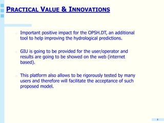
![3
2
1
segment 1
segment 2
Br
original signal
de-noised signal---------------
---------------
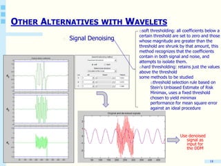
Brief analysis:
segment 1: if we observe the original signal
along this segment [140, 260], discharge is
increasing as a rainfall response somewhere,
so errors are more prone to occur during these
period and they are going to be higher in
magnitude, this is observed in the detail part
of the signal, small values are considered as
noise and they are going to be removed by
the threshold criteria. (obs: high values in
details do not mean high error or high noise)
segment2: during low flows and no flows
egment 1
higher reduction of noises
along the segment
original signal
denoised signal---------------
---------------
t 2
along this segment [140, 260], discharge is
increasing as a rainfall response somewhere,
so errors are more prone to occur during these
period and they are going to be higher in
magnitude, this is observed in the detail part
of the signal, small values are considered as
noise and they are going to be removed by
the threshold criteria. (obs: high values in
details do not mean high error or high noise)
segment2: during low flows and no flows
noises are going to be smaller and they are
also reflected in the details, the threshold
criteria is not finding errors or noise to
suppress.
low or zero reduction of
noises along the segment
2nd segment](https://image.slidesharecdn.com/test-150401081531-conversion-gate01/85/Test-13-320.jpg)
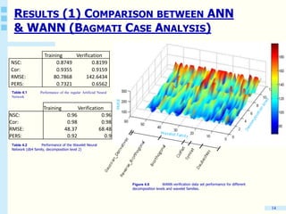
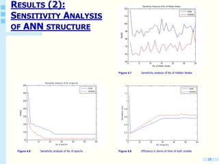
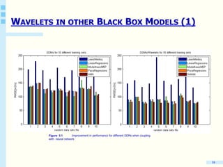
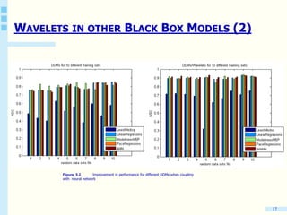
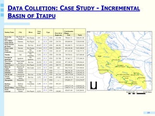
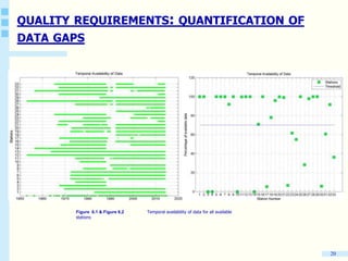
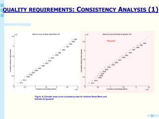
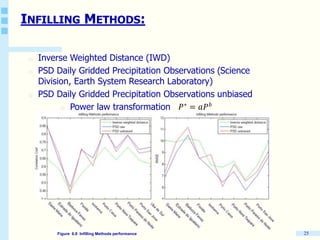
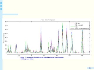
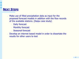
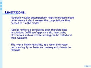

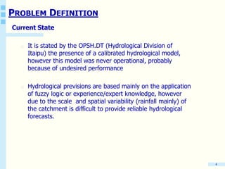
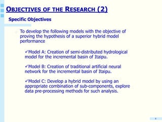
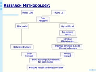
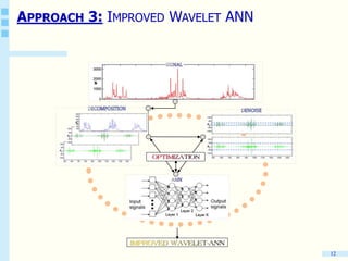
This document outlines a research project to develop improved models for forecasting reservoir inflows in the incremental basin of Itaipu using data-driven and hybrid techniques. The objectives are to create semi-distributed hydrological, artificial neural network, and hybrid models and evaluate their performance on short and medium term predictions. Methodologies include wavelet decomposition of inputs to ANNs, sensitivity analysis of ANN structures, and data preprocessing. Results will be made available through an internet-based platform to aid operational forecasting and allow further testing. Limitations include increased computational time for wavelet-ANN models and data availability challenges.


![Polymer [ बहुलक ] Chemistry Notes PDF - Irfanullah Mehar - JJ Sir Chemistry.pdf](https://cdn.slidesharecdn.com/ss_thumbnails/polymerchemistrynotespdf-irfanullahmehar-jjsirchemistry-260210172118-3f9b37f7-thumbnail.jpg?width=640&height=640&fit=bounds)


