Supervised learning algorithms learn from labeled training data to make predictions or classifications

1. Supervised Learning

2. Machine learning
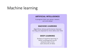
• Machine learning (ML) is defined as a discipline of artificial
intelligence (AI) that provides machines the ability to
automatically learn from data and past experiences to
identify patterns and make predictions with minimal
human intervention.

3. Learning

4. Machine learning

5. Machine Learning Model

6. How Supervised Learning Works?
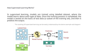
In supervised learning, models are trained using labelled dataset, where the
model learns about each type of data. Once the training process is completed, the
model is tested on the basis of test data (a subset of the training set), and then it
predicts the output.

9. Machine learning (ML)
• Machine learning (ML) is a subset of artificial intelligence (AI) that
allows machines to learn and improve from data without being
explicitly programmed. Classical ML is often categorized by how an
algorithm learns to become more accurate in its predictions. The
four basic types of ML are
• supervised learning
• unsupervised learning
• semisupervised learning
• reinforcement learning.

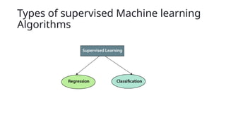
10. Supervised Machine Learning
• Supervised learning is the types of machine learning in
which machines are trained using well "labelled" training
data, and on basis of that data, machines predict the output.
The labelled data means some input data is already tagged
with the correct output.
• Supervised learning is a process of providing input data as
well as correct output data to the machine learning model.
The aim of a supervised learning algorithm is to find a
mapping function to map the input variable(x) with the
output variable(y).

11. Steps Involved in Supervised Learning
• First Determine the type of training dataset
• Collect/Gather the labelled training data.
• Split the training dataset into a training dataset, test dataset, and
validation dataset.
• Determine the input features of the training dataset, which should have
enough knowledge so that the model can accurately predict the output.
• Determine the suitable algorithm for the model, such as support vector
machine, decision tree, etc.
• Execute the algorithm on the training dataset. Sometimes we need
validation sets as the control parameters, which are the subset of training
datasets.
• Evaluate the accuracy of the model by providing the test set. If the model
predicts the correct output, it means our model is accurate.

12. Types of supervised Machine learning
Algorithms

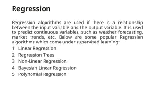
13. Regression
Regression algorithms are used if there is a relationship
between the input variable and the output variable. It is used
to predict continuous variables, such as weather forecasting,
market trends, etc. Below are some popular Regression
algorithms which come under supervised learning:
1. Linear Regression
2. Regression Trees
3. Non-Linear Regression
4. Bayesian Linear Regression
5. Polynomial Regression

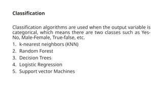
14. Classification
Classification algorithms are used when the output variable is
categorical, which means there are two classes such as Yes-
No, Male-Female, True-false, etc.
1. k-nearest neighbors (KNN)
2. Random Forest
3. Decision Trees
4. Logistic Regression
5. Support vector Machines

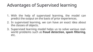
15. Advantages of Supervised learning
1. With the help of supervised learning, the model can
predict the output on the basis of prior experiences.
2. In supervised learning, we can have an exact idea about
the classes of objects.
3. Supervised learning model helps us to solve various real-
world problems such as fraud detection, spam filtering,
etc.

16. Disadvantages of supervised learning
1. Supervised learning models are not suitable for handling
the complex tasks.
2. Supervised learning cannot predict the correct output if
the test data is different from the training dataset.
3. Training required lots of computation times.
4. In supervised learning, we need enough knowledge about
the classes of object.

17. Classification
Classification algorithms are used when the output variable is
categorical, which means there are two classes such as Yes-
No, Male-Female, True-false, etc.
1. k-nearest neighbors (KNN)
2. Random Forest
3. Decision Trees
4. Logistic Regression
5. Support vector Machines

18. k-nearest neighbors (KNN)
• K-Nearest Neighbour is one of the simplest Machine Learning algorithms based on
Supervised Learning technique.
• K-NN algorithm assumes the similarity between the new case/data and available cases and
put the new case into the category that is most similar to the available categories.
• K-NN algorithm stores all the available data and classifies a new data point based on the
similarity. This means when new data appears then it can be easily classified into a well
suite category by using K- NN algorithm.
• K-NN algorithm can be used for Regression as well as for Classification but mostly it is used
for the Classification problems.
• K-NN is a non-parametric algorithm, which means it does not make any assumption on
underlying data.
• It is also called a lazy learner algorithm because it does not learn from the training set
immediately instead it stores the dataset and at the time of classification, it performs an
action on the dataset.

19. KNN algorithm
The K-NN working can be explained on the basis of the below algorithm:
Step-1: Select the number K of the neighbors
Step-2: Calculate the Euclidean distance of K number of neighbors
Step-3: Take the K nearest neighbors as per the calculated Euclidean distance.
Step-4: Among these k neighbors, count the number of the data points in each
category.
Step-5: Assign the new data points to that category for which the number of the
neighbor is maximum.
Step-6: Our model is ready.

20. k-nearest neighbors (KNN)

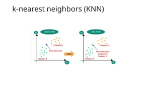
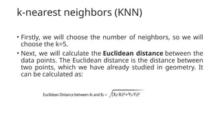
21. k-nearest neighbors (KNN)
• Firstly, we will choose the number of neighbors, so we will
choose the k=5.
• Next, we will calculate the Euclidean distance between the
data points. The Euclidean distance is the distance between
two points, which we have already studied in geometry. It
can be calculated as:

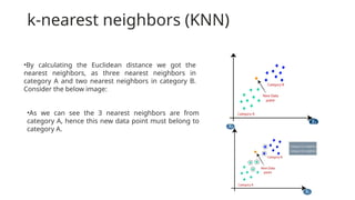
22. k-nearest neighbors (KNN)
•By calculating the Euclidean distance we got the
nearest neighbors, as three nearest neighbors in
category A and two nearest neighbors in category B.
Consider the below image:
•As we can see the 3 nearest neighbors are from
category A, hence this new data point must belong to
category A.

23. KNN
• Advantages of KNN Algorithm
1. It is simple to implement.
2. It is robust to the noisy training data
3. It can be more effective if the training data is large.
• Disadvantages of KNN Algorithm
1. Always needs to determine the value of K which may be complex some
time.
2. The computation cost is high because of calculating the distance
between the data points for all the training samples.
• Link: https://www.javatpoint.com/k-nearest-neighbor-algorithm-for-machine-
learning

24. Decision Tree
• Decision Tree is a Supervised learning technique that can
be used for both classification and Regression problems, but
mostly it is preferred for solving Classification problems.
• It is a tree-structured classifier, where
• internal nodes represent the features of a dataset,
branches represent the decision rules
• and each leaf node represents the outcome.

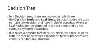
25. Decision Tree
• In a Decision tree, there are two nodes, which are
the Decision Node and Leaf Node. Decision nodes are used
to make any decision and have multiple branches, whereas
Leaf nodes are the output of those decisions and do not
contain any further branches.
• It is called a decision tree because, similar to a tree, it starts
with the root node, which expands on further branches and
constructs a tree-like structure.

26. Decision Tree

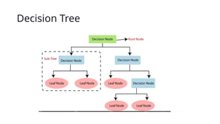
27. Decision Tree Terminologies
1. Root Node: Root node is from where the decision tree
starts. It represents the entire dataset, which further gets
divided into two or more homogeneous sets.
2. Leaf Node: Leaf nodes are the final output node, and the
tree cannot be segregated further after getting a leaf node.
3. Splitting: Splitting is the process of dividing the decision
node/root node into sub-nodes according to the given
conditions.
4. Branch/Sub Tree: A tree formed by splitting the tree.
5. Pruning: Pruning is the process of removing the unwanted
branches from the tree.
6. Parent/Child node: The root node of the tree is called the
parent node, and other nodes are called the child nodes.

28. Decision Tree Example

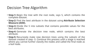
29. Decision Tree Algorithm
• Step-1: Begin the tree with the root node, says S, which contains the
complete dataset.
• Step-2: Find the best attribute in the dataset using Attribute Selection
Measure (ASM).
• Step-3: Divide the S into subsets that contains possible values for the
best attributes.
• Step-4: Generate the decision tree node, which contains the best
attribute.
• Step-5: Recursively make new decision trees using the subsets of the
dataset created in step -3. Continue this process until a stage is reached
where you cannot further classify the nodes and called the final node as
a leaf node.

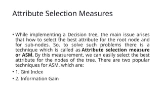
30. Attribute Selection Measures
• While implementing a Decision tree, the main issue arises
that how to select the best attribute for the root node and
for sub-nodes. So, to solve such problems there is a
technique which is called as Attribute selection measure
or ASM. By this measurement, we can easily select the best
attribute for the nodes of the tree. There are two popular
techniques for ASM, which are:
• 1. Gini Index
• 2. Information Gain

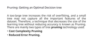
31. Pruning: Getting an Optimal Decision tree
A too-large tree increases the risk of overfitting, and a small
tree may not capture all the important features of the
dataset. Therefore, a technique that decreases the size of the
learning tree without reducing accuracy is known as Pruning.
There are mainly two types of tree pruning technology used:
• Cost Complexity Pruning
• Reduced Error Pruning.

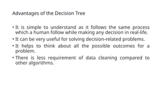
32. Advantages of the Decision Tree
• It is simple to understand as it follows the same process
which a human follow while making any decision in real-life.
• It can be very useful for solving decision-related problems.
• It helps to think about all the possible outcomes for a
problem.
• There is less requirement of data cleaning compared to
other algorithms.

33. Disadvantages of the Decision Tree
• The decision tree contains lots of layers, which makes it
complex.
• It may have an overfitting issue, which can be resolved
using the Random Forest algorithm.
• For more class labels, the computational complexity of the
decision tree may increase.

34. Support Vector Machine Algorithm
(SVM)
• Support Vector Machine or SVM is one of the most popular
Supervised Learning algorithms, which is used for
Classification as well as Regression problems.
• The goal of the SVM algorithm is to create the best line or
decision boundary that can segregate n-dimensional space
into classes so that we can easily put the new data point in
the correct category in the future. This best decision
boundary is called a hyperplane.

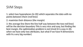
35. SVM Steps
1. select two hyperplanes (in 2D) which separates the data with no
points between them (red lines)
2. maximize their distance (the margin)
3. the average line (here the line half way between the two red lines)
will be the decision boundary This is very nice and easy, but finding the
best margin, the optimization problem is not trivial (it is easy in 2D,
when we have only two attributes, but what if we have N dimensions
with N a very big number)

36. SVM

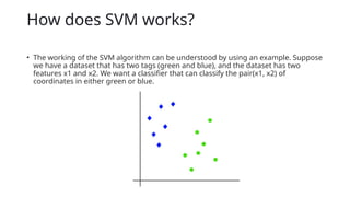
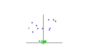
37. How does SVM works?
• The working of the SVM algorithm can be understood by using an example. Suppose
we have a dataset that has two tags (green and blue), and the dataset has two
features x1 and x2. We want a classifier that can classify the pair(x1, x2) of
coordinates in either green or blue.

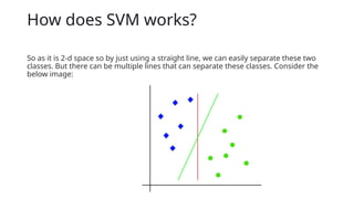
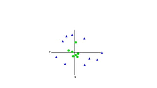
38. How does SVM works?
So as it is 2-d space so by just using a straight line, we can easily separate these two
classes. But there can be multiple lines that can separate these classes. Consider the
below image:

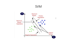
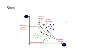
39. How does SVM works?
• Hence, the SVM algorithm helps to find the best line or decision
boundary; this best boundary or region is called as a hyperplane.
• SVM algorithm finds the closest point of the lines from both the classes.
These points are called support vectors.
• The distance between the vectors and the hyperplane is called as margin.
And the goal of SVM is to maximize this margin. The hyperplane with
maximum margin is called the optimal hyperplane.
• Support Vectors: Support vectors are the closest data points to the
hyperplane, which makes a critical role in deciding the hyperplane and
margin.

40. SVM

41. Types of Support Vector Machine
• Based on the nature of the decision boundary, Support Vector Machines (SVM)
can be divided into two main parts:
• Linear SVM: Linear SVMs use a linear decision boundary to separate the data
points of different classes. When the data can be precisely linearly separated,
linear SVMs are very suitable. This means that a single straight line (in 2D) or a
hyperplane (in higher dimensions) can entirely divide the data points into their
respective classes. A hyperplane that maximizes the margin between the classes
is the decision boundary.
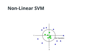
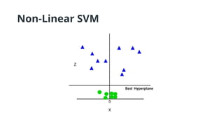
• Non-Linear SVM: Non-Linear SVM can be used to classify data when it cannot be
separated into two classes by a straight line (in the case of 2D). By using kernel
functions, nonlinear SVMs can handle nonlinearly separable data. The original
input data is transformed by these kernel functions into a higher-dimensional
feature space, where the data points can be linearly separated. A linear SVM is
used to locate a nonlinear decision boundary in this modified space.

42. Advantages of SVM
• Effective in high-dimensional cases.
• Its memory is efficient as it uses a subset of training points
in the decision function called support vectors.
• Different kernel functions can be specified for the decision
functions and its possible to specify custom kernels.

44. Non-Linear SVM

46. Non-Linear SVM

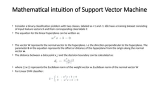
47. Mathematical intuition of Support Vector Machine
• Consider a binary classification problem with two classes, labeled as +1 and -1. We have a training dataset consisting
of input feature vectors X and their corresponding class labels Y.
• The equation for the linear hyperplane can be written as:
• The vector W represents the normal vector to the hyperplane. i.e the direction perpendicular to the hyperplane. The
parameter b in the equation represents the offset or distance of the hyperplane from the origin along the normal
vector w.
• The distance between a data point x_i and the decision boundary can be calculated as:
• where ||w|| represents the Euclidean norm of the weight vector w. Euclidean norm of the normal vector W
• For Linear SVM classifier :