Download to read offline


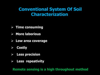
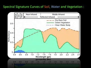
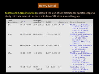
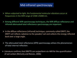
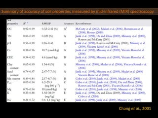
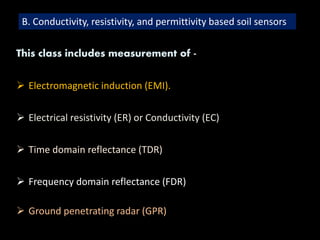
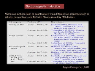
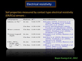
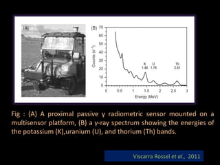
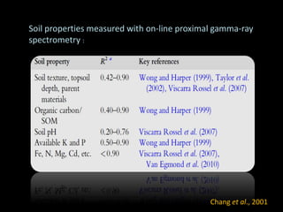
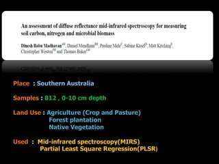
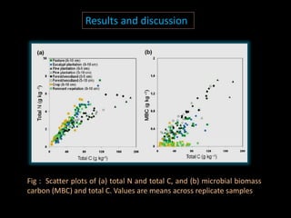
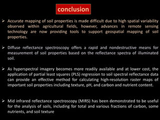


The document discusses recent developments in the sensing of soil properties, highlighting the limitations of conventional soil characterization methods and the advantages of remote sensing techniques. It covers various sensing technologies including visible-near infrared spectroscopy, mid-infrared spectroscopy, and passive radiometric sensing, emphasizing their accuracy in measuring soil properties like moisture content, organic matter, and texture. Additionally, it points out that advancements in hyperspectral imagery and data analysis methods can enhance soil property mapping despite challenges in spatial variability.


