1) The document examines how central banks balance inflation/output targets with costly sterilization of capital inflows. When sterilization costs rise, central banks limit sterilization, allowing exchange rates to adjust. 2) Empirical tests on developing countries from 1984-1992 confirm monetary policy responds to higher sterilization costs by allowing greater exchange rate changes. However, other model predictions have mixed results depending on how endogeneity is treated. 3) A theoretical model shows that higher sterilization costs are incorporated into central bank decisions as they impact the consolidated public sector budget constraint. This leads central banks to limit sterilization and tolerate more exchange rate movement.

1. Sterilization costs and exchange rate targeting∗
Kenneth Kletzer Mark M. Spiegel†
April 3, 2000
Abstract
This paper examines the movements of exchange rates and capital in-
flows in an environment where an optimizing central bank pursuing the
joint goals of inflation and output targeting engages in costly sterilization
activities. Our results predict that when faced with increased sterilization
costs, the central bank will choose to limit its sterilization activities allowing
target variables, such as the nominal exchange rate, to adjust.
We then test the predictions of a linearized version of the saddle-path
solution to the model for a cross-country panel of developing countries. We
use IV, GMM and simultaneous equation specifications to allow for the
endogeneity of capital inflows. Our results confirm that monetary policy
does respond to sterilization costs.
J.E.L. Classification Number: F32
Keywords: Sterilization, capital inflows, exchange rates
∗
Send correspondence to Mark M. Spiegel, Economic Research, Federal Reserve Bank of San
Francisco, 101 Market St., San Francisco, CA, 94105, mark.spiegel@sf.frb.org, (415)-974-3241.
†
Warren Chiang and Laura Haworth provided excellent research assistance.We thank Car-
los Vegh, participants in the UCLA international economics workshop and the FRBSF-U.C.
Berkeley summer camp for helpful comments. Remaining errors are our own.

2. 1. Introduction
With the turbulent capital movements experienced by developing nations in recent
years, many nations have engaged in efforts to slow large movements of capital
into a nation. There are a number of reasons why nations resist capital inflow
surges. First, there are a number of concerns about the implications of capital
inflows for macro variables. Under fixed exchange rate regimes, capital inflows
can be inflationary, as prices of domestic non-tradables are bid up in the wake of a
capital inflow surge. There are also concerns about movements in real exchange
rates, growth in the money stock, and a deterioration of the current account
[Calvo, Leiderman and Reinhart ([5], 1996)].
Second, there are concerns about the impact of these flows on domestic finan-
cial markets. There is a suspicion that large capital inflows may leave a nation
exposed to rapid capital outflows: some capital inflows may be in the form of ”hot
money,” whose owners are likely to flee at the first sign of difficulty. Another
source of instability is that a nation may have difficulty allocating very rapid
capital inflows into their most productive uses. This may lead to poor invest-
ment decisions and bankruptcy in the wake of the inflow surge. This problem is
particularly severe for developing countries, whose financial sectors are relatively
unsophisticated.
Finally, governments may wish to limit the magnitude of a capital inflow surge
because of moral hazard difficulties. Investors may be willing to invest in even
poor projects in a developing country if they perceive some sort of government
guarantee of their return on their project. Indeed, the onset of the perception
that these government guarantees were not credible has been raised as one source
2

3. of the Asian currency crisis [Burnside, et al, ([1], 1998)].
The choices available to policy makers wishing to stem capital inflows are
limited. Policy makers confronted with a surge in capital inflows can either im-
plement some form of capital control, through either a quantitative restriction on
inward capital movements or a tax on these movements, or attempt to mitigate
the inflationary impact of these capital flows by sterilized exchange rate interven-
tion. Sterilization is usually the first policy response to a sudden rise in financial
capital inflows. Under this policy, central banks swap domestic securities, such
as government treasury obligations, for incoming foreign assets. The net impact
of a sterilization exercise is that the monetary base is unchanged, but the share
of foreign reserves in central bank asset holdings have increased.1
A number of studies [e.g. Calvo, Leiderman and Reinhart ([4], 1993) and
Frankel and Okongwu ([10], 1996)] question both the feasibility and desirability
of sterilization efforts. Drawing on warnings initially raised by Calvo ([3], 1991),
these studies argue that there are ”quasi-fiscal” costs associated with sterilization
as central banks exchange high-yielding domestic government debt for foreign
securities typically paying lower nominal yields.
Estimates of quasi-fiscal costs based on observed spreads between domestic
and foreign assets and the size of foreign reserve increases for developing country
central banks engaging in sterilization activities indicate that these costs can
become large. Calvo, et al ([4], 1993) and Khan and Reinhart ([12], 1994) report
1
More draconian forms of limiting capital inflows include raising bank reserve requirements or
taxing international capital movements. See Spiegel ([20], 1995) and Reinhart and Smith ([18],
1998) respectively for discussions of adverse macroeconomic implications of these alternative
instruments.
3

4. estimates for Latin America between 0.25 and 0.5 percent of GDP. Kletzer and
Spiegel ([13], 1998) report estimates of quasi-fiscal costs for the Pacific Basin
nations with similar average magnitudes, but their results suggest that capital
inflow surges can result in quarterly peaks above one percent of GDP for nations
such as Singapore and Taiwan. However, Kletzer and Spiegel caution that these
are ”upper-bound” estimates of the magnitude of quasi-fiscal costs, since domestic
bond spreads can incorporate true default risk premia.
As a result, there are many sources of exchange rate premia under which
uncovered interest rate parity is maintained. For example, Craine ([6], 1999) has
demonstrated that an exchange rate premium will exist when governments lack
complete credibility in maintaining a nominal exchange rate peg, even in cases
where the exchange rate regime is fundamentally sound in the sense of the central
bank possessing adequate reserves to defend the announced peg. The reason is
that there is a true possibility of ending up in an equilibrium in which the peg
is not defended, even if its defense is feasible. A bond spread stemming from
sovereign risk of this type does not represent a true deviation from interest rate
parity.
Alternatively, one could turn to asymmetric information as a source of a true
deviation from interest rate parity. Consider a government that knows that it is a
good credit risk, but is pooled with a number of nations that are poor credit risks
because of information costs. Such an outcome would represent a true deviation
from interest rate parity, and the government would correctly consider a swap of
domestic for foreign debt as costly.
This paper considers the decision problem for a rational central bank faced
with a deviation from interest rate parity corrected for default risk, so that steril-
4

5. ization is costly. The central bank chooses the exchange rate as its instrument of
optimal policy. Other models which consider optimal sterilization policy include
Roubini ([19], 1988) which considers optimal sterilization policies in a static set-
ting, and Natividad and Stone ( [15], 1990), which consider optimal policies under
imperfect capital mobility. Our model differs from the latter by explicitly incor-
porating the implications of sterilization policy for the consolidated government
budget constraint into the central bank’s decision problem.2
The paper therefore follows the literature which models speculative attacks
on exchange rate regimes based on endogenous rational central bank policies, e.g.
Obstfeld ([16], 1986) and ([17], 1995) and Buiter ([2], 1987)]. This is distinct from
the classical speculative attack literature, exemplified by Krugman ([14], 1979)
and Flood and Garber ([8], 1984a), ( [9], 1984b), in which the process of domestic
credit creation is taken as exogenous.
We use a model of exchange rate determination for a small open economy in
which domestic monetary policy is set by an optimizing central bank in an envi-
ronment in which sterilization is costly. To obtain short-term non-neutrality, we
introduce wage stickiness. The central bank then chooses the nominal exchange
rate so as to minimize movements in the nominal rate and deviations from its out-
put target. As in Buiter ([2], 1987), this optimal policy is chosen subject to an
inter-temporal budget constraint. Our results demonstrate that the costs of ster-
ilization, which impact on the inter-temporal budget constraint, are incorporated
by the central bank in its monetary policy decisions.
We then test the predictions of the saddle-path stable solution of the model
2
Also, see Daniels ([7], 1997) for a consideration of strategic determinants of sterilization
activity in a two-country framework.
5

6. for a panel of 24 ”dirty-floating” nations during the high capital-inflow period
from 1984 through 1992. We use IV, GMM and simultaneous equation spec-
ifications to allow for the endogeneity of capital inflows. Our results strongly
confirm the primary implication of the theory that monetary policy does respond
to sterilization costs. In particular, increased sterilization costs are shown to be
positively associated with increases in the rate of change in the nominal exchange
rate. However, other aspects of the model yield mixed results. The significance
of predictions of the theoretical model for coefficient values are found to be sen-
sitive to our treatment for endogeneity, and cross-coefficient restrictions implied
by the strong functional form of the theory are rejected by the data.
2. Capital inflows and optimal central bank intervention
2.1. Exchange rate determination under nominal wage rigidity
We begin with a standard monetary model of the exchange rate with nominal wage
rigidities. All variables, except domestic and foreign interest rates, are expressed
in logarithms. We assume that the log of aggregate supply, yt, is an increasing
function of the inverse of real wages and is subject to an identical independent
zero mean shock, ut, each period:
yt = α(pt − wt) + ut, (2.1)
where wt is the average wage rate, pt is the price level, and α is an exogenous
constant.
We assume that all agents in the economy are rational and sign one-period
nominal wage contracts for the following period. We normalize equilibrium full-
6

7. employment output to unity, so that
wt = Et−1pt and Et−1yt = 0. (2.2)
Equilibrium in the money market is assumed to be given by
mt − pt = ϕyt − δit+1 + νt, (2.3)
where mt is the supply of domestic currency, it+1is the interest rate prevailing on
claims held at the end of period t and νt is a possibly serially-correlated distur-
bance to money demand. We also impose purchasing power parity,
st + p∗
t = pt; (2.4)
where st is the spot exchange rate (in logs) expressed as units of domestic currency
per unit of foreign currency.
As we noted in the introduction, we assume that uncovered interest rate parity
fails to hold. Define γt as the deviation from uncovered interest rate parity on
public debt denominated in domestic currency. Assuming that the true proba-
bility of default on government debt is zero, γt satisfies
it+1 = i∗
t+1 + (Etst+1 − st) + γt, (2.5)
The foreign price level is held constant and normalized to one for simplicity (p∗
t =
0). Combining these relationships leads to the exchange rate equation,
st = Ω−1
(mt + δ i∗
t+1 + γt − νt) + αϕEt−1st − ϕut + δEtst+1 . (2.6)
where Ω is the constant term
Ω = 1 + δ + αϕ
7

8. This can be solved forward ruling out speculative bubbles by imposing the con-
dition,
lim
v→∞
δ
1 + δ
v−t
Etsv+1 = 0,
to obtain the exchange rate equation,
st = Ω−1



mt + Et


∞
j=t+1
δ
1 + δ
j−t
mj + δ(i∗
j + γj) − vj

 + ϕ (αwt − ut)



.
(2.7)
2.2. Central bank decision problem
The central bank’s decision problem is to choose the spot rate to minimize an
inter-temporal quadratic loss function defined over movements in the nominal
exchange rate and deviations from y∗
, a target level for output,
Lt =
1
2
Et
∞
s=t
βs−t
θ (st − st−1)2
+ (yt − y∗
)2
. (2.8)
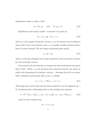
subject to the inter-temporal budget constraint for the consolidated government.3
The single-period budget identity is given in levels (not logarithms) by
Bt = (1 + it)Bt−1 + Gt + [StRt − (1 + i∗
t )StRt−1 − (Mt − Mt−1)] , (2.9)
where Bt, Rt and Mt are stocks of privately-held public debt, central bank reserves
and base money at the end of period t. Gt is consolidated primary deficit of the
public sector for period t, and St is the spot exchange rate in period t. The term
3
We model the central bank decision problem as the choice of the nominal spot rate for
simplicity. Operationally, the central bank may be seen as conducting monetary policy which
is consistent with its chosen spot exchange rate.
8

9. in square brackets is the transfer from the central bank to the fiscal authority in
units of domestic currency.
A capital inflow during period t leads to an increase in foreign reserves given
by ∆Rt ≡ (Rt − Rt−1). The appropriate discount factor to apply to future public
sector budget surpluses equals
It,t+j =
t+j
i=t+1
1
(1 + ii)
. (2.10)
We also impose the conventional solvency condition on the public sector,
lim
T→∞
Et ΠT
j=t (1 + ij)−1
BT = 0. (2.11)
Sterilization of a capital inflow at date t leads to a present value increase in
future surpluses inclusive of monetization necessary to maintain public sector sol-
vency if γt excludes, as we assume here, any correctly-priced default risk premium.
The present value cost of sterilizing a capital inflow of size ∆Rt is
Et
∞
j=1
It,t+j γt+jSt∆Rt . (2.12)
Unless the government cuts expenditures or increases taxes, the net cost of ster-
ilization must eventually be monetized.
If the date t capital inflow is fully monetized at time t + T, then public sector
solvency is maintained if the date t + T increase in the domestic money supply
equals
Mt+T − Mt+T −1 = St∆Rt + Et
T
j=1
γt+jSt∆Rt
t+j
i=t+1
(1 + ii) , (2.13)
the initial capital inflow in domestic currency plus the accumulated costs of ster-
ilized intervention. The date t present value of future monetization at date t + T
9

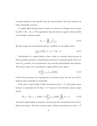
10. is
(Mt+T − Mt+T−1) It,t+T = St∆Rt + Et
T
j=1
It,t+j γt+jSt∆Rt , (2.14)
which grows with the horizon T for positive γt+j. The costs of sterilization at
date t can also be continuously monetized through monetary expansions equal to
γsSt∆Rt at every date s > t. Without sterilization costs (γt = 0), the expected
future money supply increase needed to maintain public sector solvency after a
sterilized capital inflow is zero.
If a capital inflow of size ∆Rt is not sterilized, the currency depreciates at date
t by the amount
∆st = Ω−1 St∆Rt
Mt−1
, (2.15)
using equation 2.7. Sterilization at date t followed by the eventual monetization
of the resulting increase in public debt at time t+T leads to a depreciation of the
home currency at time t + T given by
∆st+T = Ω−1


St∆Rt
Mt+T−1
+
T
j=1
γt+jSt∆Rt
Mt+T−1
t+j
i=t+1
(1 + ii)

 . (2.16)
The currency also depreciates at date t given future monetization by the amount
∆st = Et
δ
1 + δ
T
∆st+T . (2.17)
Sterilization therefore has the same effect as borrowing reserves. It postpones
an eventual depreciation or fiscal contraction. With an public debt interest pre-
mium, sterilization leads to a larger future depreciation and a current depreciation.
Buiter ([2], 1987) shows how borrowing reserves can either postpone or advance
the date of an eventual speculative attack under a pegged exchange rate. In his
model, there are no costs to sterilization; foreign currency denominated public
10

11. debt will pay the same rate of interest as foreign public debt. Applying our model
to a collapsing exchange-rate peg favors the depreciation of the shadow exchange
rate.
3. Solution for the optimum
Define µt as the ratio of real balances to output
µt ≡
Mt−1
PtYt
,
∆ρt as the ratio of net reserve inflows to GDP
∆ρt ≡
StRt − (1 + i∗
t )StRt−1
PtYt
,
and bt as the outstanding public debt to GDP ratio
bt ≡
Bt
PtYt
.
Inter-temporal optimization by the central bank then leads to the Euler con-
dition,
qt = βEt [(1 + i∗
t + γt)qt+1] , (3.1)
where qt is the costate variable associated with the public sector budget constraint.
The necessary conditions include
qt =
θ (st − st−1) + α (yt − y∗
)
Ωµt
(3.2)
and the transversality condition
lim
t→∞
βt
qtbt = 0. (3.3)
11

12. To derive a relationship between capital inflows and the exchange rate, we
linearize about the deterministic steady state. This is given by
q = 0, (3.4)
wt = st−1 +
α
θ
y∗
, (3.5)
∆st = (st − st−1) =
α
θ
y∗
(3.6)
and
b = (1 + i∗ + γ)b + g + ∆ρ − µ (st − st−1) , (3.7)
where gt is the primary deficit to GDP ratio (g is the ratio in the deterministic
steady state).
Linearization of the dynamics about the steady state gives
dqt = βEt (1 + i∗ + γ)dqt+1 + d(i∗
t+1 + γt+1)dqt+1) , (3.8)
where the differential operator is used to denote deviations from deterministic
steady-state values (dxt ≡ xt − x). This becomes upon substitution
∆st = β(1 + i∗ + γ)Et [∆st+1] + βσsi, (3.9)
treating the correlation between the rate of nominal depreciation and the foreign
rate of interest inclusive of premium,
σsi = Et ∆st+1d(i∗
t+1 + γt+1) ,
as a constant evaluated in the stochastic stationary state. Note that at the steady
state
d∆st = ∆st
12

13. and
dqt =
α2
+ θ
Ωµ
d∆st.
The exchange rate equation evaluated about the steady state gives
∆st = Ω−1
{∆mt + δ∆i∗
t − (∆νt + ϕ∆ut) + δEt [∆st+1]} , (3.10)
and the budget identity becomes
dbt = (1 + i∗ + γ)dbt−1 + bd(1 + i∗
t + γt) + dgt + d∆ρt − µ∆mt. (3.11)
Substitution using the linearized Euler condition and exchange rate equation leads
to the two equation system:
Et [∆st+1] = β−1
(1 + i∗ + γ)−1
∆st − (1 + i∗ + γ)−1
σsi (3.12)
and
dbt = (1 + i∗ + γ)dbt−1 − µ Ω − δβ−1
(1 + i∗ + γ)−1
∆st (3.13)
+dgt + d∆ρt + µ [δ∆i∗
t − (∆νt + ϕ∆ut)] + bd(i∗
t + γt).
We let i∗
t , γt, ut and ∆νt all be iid4
. The saddle-path stable solution satisfying
the transversality condition is given by
∆st = ψdbt−1 + Et
∞
s=t
(1 + i∗ + γ)−(s−t)
ψ (dgs + d∆ρs + εs) +
σsi
(1 + i∗ + γ)
,
where
ψ ≡


β(1 + i∗ + γ)2
− 1
µ βΩ(1 + i∗ + γ) − δ


4
As we mentioned above, the shocks to money demand νt could exhibit first-order serial
correlation.
13

14. and
εt ≡ µ [δ∆i∗
t − (∆νt + ϕ∆ut)] + bd(i∗
t + γt).
See the appendix for the details of this solution.
This implies that the change in the rate of nominal depreciation for a shock
at time t is given by
d∆st = ψ (dbt−1 + dgt + d∆ρt + εt)+ψEt
∞
s=t+1
(1+i∗ +γ)−(s−t)
(dgs + d∆ρs + εs) .
(3.14)
If we assume that shocks are i.i.d., equation 3.14 satisfies
d∆st = ψ (dbt−1 + dgt + d∆ρt + εt) . (3.15)
Alternatively, we allow the primary budget deficit, reserve inflows, and either
the first-difference in the world rate of interest or shocks to money demand to
follow a first-order autoregressive process. In particular, let dgt, ∆ρt, and εt
satisfy
dgt = η1dgt−1 + ζ1t
∆ρt = η2∆ρt−1 + ζ2t,
and
εt = η3εt−1 + ζ3t,
where 0 ≤ ηj < 1 and Et−1 ζjt = 0 (j = 1, 2, 3).
For these stationary processes, we have that
d∆st = ψ dbt−1 +
1 + i∗ + γ
1 + i∗ + γ − η1
dgt +
1 + i∗ + γ
1 + i∗ + γ − η2
d∆ρt +
1 + i∗ + γ
1 + i∗ + γ − η3
εt
(3.16)
14

15. 4. Empirical Results
4.1. Single Equation Specification
In this section, we estimate our saddle-path stable solution for i.i.d. and first-
order autoregressive shocks for a panel of dirty-floating nations. Our theory is
likely to omit a number of important country and time-specific characteristics
which also affect the path of exchange rates. We therefore introduce ξi to account
for country-specific fixed effects which are time-invariant and φt to account for
time-specific fixed effects.
By equations 3.15 and 3.16, the change in the rate of nominal exchange rate
depreciation of country i in period t satisfies
d∆st = ξi + φt + ψdbt−1 + (ψΨ1) dgt + (ψΨ2) d∆ρt (4.1)
+ (ψΨ3µδ) ∆i∗
t + ψΨ3b d(i∗
t + γt) + et
where et is the disturbance term
et = − (ψΨ3µ) (∆vit + ϕ∆uit)
and
Ψj =
1 + i∗ + γ
1 + i∗ + γ − ηj
≥ 0; (j = 1, 2, 3)
The above specification nests the specifications under the alternative assumptions
that the shocks are first-order autocorrelated and that they are i.i.d. Under both
specifications, all four coefficient values are predicted to be positive. With the
additional assumption that the shocks are i.i.d. we have the additional parameter
restriction
Ψ1 = Ψ2 = Ψ3 = 1.
15

16. We first sweep the data of its period means so that we can do away with the
time-specific effects, φt. Next, we eliminate the country-specific fixed effects by
differencing the data. We obtain
(∆si,t − ∆si,t−1) = ψ (bi,t−1 − bi,t−2) + (ψΨ1) (gi,t − gi,t−1) (4.2)
+ (ψΨ2) ∆ρit − ∆ρit−1
+ ψΨ3b γit − γit−1 + (et − et−1)
Our specification therefore predicts positive coefficients on the first differences
of the four regressors on the right-hand side. Under the assumption the shocks
are i.i.d., the model predicts an additional testable parameter restriction, namely
that the coefficients on the first three regressors are equal in magnitude. We use
this restriction to test the hypothesis of i.i.d. shocks below against the alternative
of shocks which follow a first-order autoregressive process.
The methodology to be used in estimating equation 4.2 depends on the as-
sumptions we are willing to make concerning the exogeneity of the right-hand side
variables. We first report the ordinary least squares (OLS) results for the spec-
ification above. However, these estimates will be inconsistent if the right-hand
side variables are endogenous. This would appear to be a particular problem
for the net capital inflows term, as capital inflows may respond to exchange rate
movements as a signal of future monetary policy.
We respond to the potential endogeneity problem in two ways. First, we
allow all of the right-hand-side variables to be endogenous and then instrument
for them with lagged dependent variables. This specification will be consistent
under the assumption that the right-hand-side variables are weakly exogenous,
i.e. that E(∆Xit∆ is) = 0 for all right-hand-side variables Xit for all s > t. We
16

17. then estimate the specification in an OLS instrumental variables (IV) framework
and a Generalized Method of Moments (GMM) framework. Second, we allow for
endogeneity only in the capital inflows term and provide an explicit specification
which we can estimate using a simultaneous equations framework in the following
section.
4.2. Data
We use a balanced panel of quarterly data for 24 countries from February 1984
through April 1992. The time series was chosen to correspond to a period where
countries in the sample were receiving high levels of capital inflows. Data sources
are listed in detail in the data appendix. The summary statistics for these coun-
tries are listed in Table 1.
An issue which immediately arises in Table 1 is that we are pooling across
countries which report themselves as pursuing different exchange rate regimes.
Our panel includes 7 countries which claim to have pursued a pegged regime
throughout the period and 10 which pursue a managed float throughout the pe-
riod.5
The eight remaining countries in the sample changed their designation
between pegged and floating at some point during the sample period.
Among these various country groups, the greatest concern with pooling would
arise with those which maintained a pegged regime throughout the period. Be-
cause they were attempting to maintain a peg, these countries may have been
systematically more reluctant to adjust their spot rate in the face of shocks than
5
Two of the countries switched their exchange rate regime designations during the sample
period from managed float to float. Costa Rica switched in the first quarter of 1992 while the
Philippines switched in the third quarter of 1984.
17

18. countries in a managed floating regime. However, all of these countries adjusted
their pegs over the sample period, some numerous times.
There is some reason to suspect that these countries do behave differently as
a group than their counterparts in the other groups. The average level of the
absolute value of log differences in spot exchange rates, the dependent variable
in our specification, for the 24 countries in the sample is 0.0518. In contrast, the
countries which maintained a peg throughout the sample period had an average
of 0.0198. However the countries which pursued a managed float throughout the
period were not that different, with an average log difference in the spot rate of
0.0266. It turns out that the greatest volatility was experienced in those countries
which either abandoned a peg in favor of a floating regime, or vice versa. For
these countries, the average log difference in spot rate was 0.1158. However, to
maintain a balanced panel, we classify those countries which switched between
regimes as in our ”managed floating” group.6
Finally, γit is unobservable directly because it is a function of the expected
future spot rate, as shown above in equation 2.5. Estimation of equation 4.2 then
requires some estimate of the expected future spot rate to allow us to construct an
estimate of γit. A number of different proxies have been used in the literature.7
We proceed under the assumption that agents have perfect foresight in predicting
6
To account for potential differences between these groups, we examined the robustness of
our results below to the exclusion of those countries which maintained a pegged regime for the
duration of the sample. Our results with these countries excluded were very similar to those
for the entire sample. The simultaneous equation results are reported in Table 4, while all of
the single equation results are available from the authors upon request.
7
For example, Goldberg (1994) estimates a series of rolling regressions, while Frankel and
Okongwu (1996) use survey data.
18

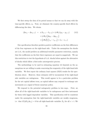
19. exchange rate changes. While this assumption is somewhat strong in levels,
we note that after differencing the panel data, which we do below to eliminate
country-specific fixed effects, the specification run is exactly equivalent to that
which would emerge under the opposite extreme assumption that agents expected
the exchange rate to follow a random walk. Our specification therefore nests
both the perfect foresight and the random walk specifications used in Kletzer and
Spiegel ([13], 1998).
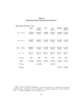
4.3. Single Equation Results
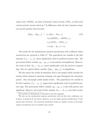
The results for the full-sample regression are shown in Table 2. The primary
result is the strong performance of the term representing the quasi-fiscal costs
of sterilization, γit − γit−1 . This term enters significant and positive for all
specifications with or without the parameter restriction implied by the assumption
that the shocks are i.i.d., i.e. the restriction that the coefficients on the first three
regressors are equal. The performance of the other three coefficients, however,
reflect varying degrees of sensitivity to our treatments for endogeneity and the
application of the i.i.d. coefficient value restriction.
With the first three parameters constrained to be equal, all three of these vari-
ables enter significantly positive, as predicted, in both the OLS and IV specifica-
tions. However, they are insignificant in the GMM specification. With the coeffi-
cient values of the first three regressors unrestricted, their performance varies. In
the OLS specification, (gi,t − gi,t−1) and ∆ρi,t − ∆ρi,t−1 enter significantly with
their predicted positive signs, but (bi,t−1 − bi,t−2) enters significantly with the in-
correct negative sign. After instrumenting, these three variables are insignificant
in both the IV and GMM specifications.
19

20. We also report the results of a formal F-test concerning the parameter restric-
tion implied by the assumption that the shocks in the model are i.i.d. For the
OLS regression, we obtain an F-statistic of 13.678 for the test of the restricted
versus unrestricted specification. This would imply a rejection of the assumption
that shocks are i.i.d. in our model in favor of our more general autoregressive
specification. However, in the IV and GMM specification, we obtained a higher
sum-of-squared errors in terms of fitting the original regressors (rather than those
fitted with our instruments) with the unrestricted specification than with the first
three coefficients restricted. Since endogeneity is a serious issue in this specifica-
tion, this provides some evidence in support of the restrictions imposed by the
assumption that the shocks are i.i.d.
The diagnostic results for the validity of the GMM specification are also pre-
sented. We find no presence of second-order serial correlation in any specification,
indicating that the Sargen statistic is a valid test of the over-identifying restric-
tions in the model. Our results from the Sargen statistic strongly fail to reject
the null hypothesis that the over-identifying restrictions in our specification are
valid.
4.4. Simultaneous Equation Specification
In this section, we examine an explicit simultaneous equation system with two en-
dogenous variables: ∆ρi,t and ∆si,t. We specify an equation for the determination
of net capital inflows using variables which are perceived as correlated with the
desirability of a nation’s assets. In addition to exchange rate movements, ∆si,t,
which might affect investor expectations concerning the path of future monetary
policy, we also specify net capital inflows as dependent upon the domestic debt-to-
20

21. export ratio, DEBTit, an index of domestic terms of trade, TOTit, as well as the
current period’s income shock yit.8
In differences with the time dummies swept,
our second equation then becomes
∆ρi,t − ∆ρi,t−1 = α1 (∆si,t − ∆si,t−1) (4.3)
+α2 (DEBTi,t − DEBTi,t−1)
+α3 (TOTi,t − TOTi,t−1)
+α4 (yi,t − yi,t−1) + uit.
The results for the simultaneous equation specification with coefficient values
unrestricted are reported in Table 3.9
The quasi-fiscal cost variable in the first
equation, γit − γit−1 , enters significantly with its predicted positive sign. The
government deficit variable, (git − git−1) , is also positive and significant. However,
the stock of debt, (bit−1 − bit−2) , enters significantly with the incorrect negative
sign. The net capital inflows variable, ∆ρit − ∆ρit−1 , is insignificant.
We also report the results of estimation with a sub-sample which excludes the
nations which claimed to maintain exchange rate pegs throughout the estimation
period. Our sub-sample yields similar results. The quasi-fiscal cost variable in
the first equation, γit − γit−1 , again enters significantly with its predicted pos-
itive sign. The government deficit variable, (git − git−1) , is also still positive and
significant. However, the stock of debt variable, (bit−1 − bit−2) , now fails to enter
8
The method of calculating yit is described in the data appendix.
9
We also ran the simultaneous equation specification with the first three coefficients con-
strained, as predicted by the theory. However, as in the single equation specifications, F-tests
rejected this restriction. The restricted specification results are similar to those in the single-
equation specification and are available upon request.
21

22. significantly. The net capital inflows variable, ∆ρit − ∆ρit−1 , is insignificant as
before, but now enters with its predicted positive point estimate.
For completeness, we also report the results of the second regression, the de-
terminants of the magnitude of capital inflows. As expected, the difference in the
rate of exchange rate depreciation, (∆sit − ∆sit−1) , is a very significant predic-
tor of the level of capital inflows, suggesting that net capital inflows are indeed
endogenous. Income shocks, (yit − yit−1) , are also significantly positive, as would
be expected. The stock of debt is significantly negative, as would be expected.
Finally, the terms of trade variable fails to enter significantly. The results with the
omission of the pegged countries from the sample are similar, with the exception
that the change in the stock of debt fails to enter significantly.
5. Conclusion
Our theoretical results demonstrate that a forward-looking central bank will incor-
porate sterilization costs in its monetary policy decisions, choosing more accom-
modating nominal exchange rate strategies the higher is the cost of maintaining
an announced peg or crawl. Our empirical results support this claim. Using a
specification which directly follows the linearized decision rule from the theory,
we confirm that the central banks in our panel of 24 developing countries during
a period of high capital inflows did respond to sterilization costs in their nominal
exchange rate policy.
The importance of these costs in central bank decisions, however, still comes
down to the level of true deviations from interest rate parity. As we suggested
in the introduction, our estimates of deviations from interest rate parity in these
22

23. countries must represent upper bounds, as some portion of the spread paid on
domestic securities over foreign assets must represent true differences in default
risk. To the extent that spreads represent true default risk premia, rather than
deviations from interest rate parity, actual sterilization costs are reduced.
However, it is clear that developing country governments do behave as if steril-
ization is a costly process. Most countries only attempt sterilization over limited
periods, eventually choosing to either accommodate the capital inflow through an
expansion of the domestic money supply or through an appreciation of the nom-
inal exchange rate. The limited duration of sterilization programs suggest that
the costs considered in this paper are incorporated into central bank decisions.
23

24. 6. Appendix
The eigenvalues of the solution for the optimum are
λ1 = (1 + i∗ + γ)
and
λ2 = β−1
(1 + i∗ + γ)−1
,
and the eigenvectors are
υ1 =
E∆s
db = 0
1
and
υ2 =
E∆s
db = ψ
1 =
β−1
(1+i∗+γ)−1−(1+i∗+γ)
µ[−(1+δ+αϕ)+δβ−1
(1+i∗+γ)−1
]
1
The saddle-path stable solution which satisfies the transversality condition is
then given by
Et∆st+1
dbt
=
β−1
(1 + i∗ + γ)−1
0
−µ (1 + δ + αϕ) − δβ−1
(1 + i∗ + γ)−1
(1 + i∗ + γ)
∆st
dbt−1
+
−(1 + i∗ + γ)−1
σsi
dgt + d [∆ρt] + µ [δ∆i∗
t − (∆νt + ϕ∆ut)] + bd(1 + i∗
t + γt)
24

25. 7. Data Appendix
Data is quarterly from the second quarter of 1984 through the fourth quarter of
1992. For all countries other than Taiwan, the following data was obtained from
the International Monetary Fund’s International Financial Statistics: exchange
rate, line ae; nominal GDP, line 99b; real GDP, line 99bp; government deficit, line
80 (except as noted below); exports, line 70d; government bonds, line 32an; foreign
reserves, line11; three month interest rates, line 60c where available (exceptions
are noted below); CPI, line 64. Interpolated annual nominal GDP data (line
99b) was used except for: Mexico, Israel, Korea, Philippines and Taiwan, which
had quarterly data available. Data for these variables for Taiwan was obtained
from Financial Statistics, Taiwan District. The terms of trade index is annual
data obtained from the Penn World Tables. Annual foreign debt data is from the
World Bank STARS database, except Israel, which is from Government Finance
Statistics. Annual data was interpolated into quarterly frequencies.
Countries for which line 60c were not available include Argentina (60b), Bolivia
(60p), Chile (60p), Costa Rica (60), Honduras (61), Venezuela (61), India (60b),
Korea (60b), Pakistan (60b), Mauritius (60b). Some missing observations were
interpolated. Details are available from the authors. Interest rate data for
Taiwan was 31-90 day commercial paper rate from Financial Statistics, Taiwan
District. Interest rate data for Indonesia was obtained from Bank of Indonesia.
Data for Malaysia and Thailand were 3 month T-bill and lending rate average
respectively, obtained from DRI.
Annual government deficit data was interpolated into quarterly data over some
range for Bolivia, Chile, Honduras, Israel, Sri Lanka, India, Pakistan, Mauritius,
Zimbabwe, Fiji, Papua New Guinea, Taiwan, and Indonesia. Further details are
available from the authors.
25

26. Table 1
Summary of Exchange Rate Regimes in the Sample10
Country Regime11
s Max s Min s ∆s Max ∆s Min ∆s
Argentina mf-f-p 0.29 1.00 5*10−6
0.36 2.80 -7*10−3
Barbados p 2.00 2.01 2.00 2*10−4
0.00 -6*10−3
Bolivia p-f 2.36 4.10 2*10−3
0.26 2.72 3*10−3
Chile mf 248.75 382.33 77.06 0.05 0.55 -0.07
Costa Rica mf-f 82.36 137.43 44.00 0.03 0.11 -0.02
Fiji p 1.35 1.56 1.07 0.01 0.18 -0.05
Honduras p-mf-f 2.78 5.83 2.00 0.03 0.97 0.00
India mf 16.47 26.20 11.19 0.03 0.20 -0.04
Indonesia mf 1630 2062 1014 0.03 0.37 0.00
Israel mf-p 1.73 2.76 0.24 0.09 0.53 -0.05
Kenya p 21.005 36.22 14.48 0.03 0.10 -0.03
Korea mf 777.72 891.70 667.20 1*10−4
0.03 -0.06
Malawi p 2.49 4.40 1.39 0.03 0.22 -0.10
Malaysia p-mf 2.60 2.78 2.32 4*10−3
0.06 -0.05
Mauritius p 14.61 17.00 12.18 9*10−3
0.13 -0.10
Mexico mf 1.88 3.12 0.17 0.09 0.34 -2*10−3
Pakistan mf 19.56 25.70 13.98 0.02 0.07 -4*10−3
Papua N.G. p 0.93 1.02 0.83 0.01 0.13 -0.06
Philippines mf-f 22.22 28.00 18.00 0.02 0.25 -0.07
Sri Lanka mf 34.25 46.00 25.17 0.02 0.15 -2*10−3
Taiwan mf 31.04 40.40 24.65 0.01 0.03 -0.10
Thailand mf-p 25.69 27.55 23.00 3*10−3
0.17 -0.04
Venezuela p-f 30.29 79.45 7.50 0.07 0.93 0.00
Zimbabwe p 2.48 5.48 1.20 0.05 0.44 -0.05
10
Source: International Monetary Fund Exchange Rate Restrictions and Arrangements.
11
p=peg; mf=managed float; f=float
26

27. Table 2
Single-Equation Specification Results12
Dependent Variable: d∆sit:
OLS OLS IV IV GMM GMM
(Rest.) (Rest.) (Rest.)
bit−1−bit−2 −0.2213∗∗
(0.0949)
0.2131∗∗
(0.0465)
0.2629
(0.5111)
0.1712∗∗
(0.0810)
0.1203
(0.5039)
0.1474
(0.2412)
git−git−1 0.4569∗∗
(0.0814)
0.2131∗∗
(0.0465)
0.1195
(0.2025)
0.1712∗∗
(0.0810)
0.1591
(0.3222)
0.1474
(0.2412)
∆ρit − ∆ρit−1 0.3667∗∗
(0.0832)
0.2131∗∗
(0.0465)
0.1788
(0.1763)
0.1712∗∗
(0.0810)
0.2155
(0.8162)
0.1474
(0.2412)
γit − γit 2E−6∗∗
(3E−7)
2E−6∗∗
(4E−7)
3E−6∗∗
(5E−7)
3E−6∗∗
(5E−7)
3E−6∗∗
(9E−7)
3E−6∗∗
(9E−7)
# obs. 792 792 792 792 792 792
DW 0.0408 0.0401 0.0454 0.0452 0.0465 0.0458
F Test 13.6738 0.0512
Sargan 0.0104 0.0306
12
Rest. refers to restricted specification. First three reressors are restricted to have same
coefficient value. Standard errors in parentheses. * indicates significance at 10% confidence
level. ** indicates singificance at 5% confidence level.
27

28. Table 3
Simultaneous Equation Model13
Equation 1: Dependent Variable: d∆st
Full Sample Pegged Countries Omitted
bit − bit−1 −0.2223∗∗
(0.0857)
−0.1377
(0.1020)
git − git−1 0.4127∗∗
(0.0811)
0.6551∗∗
(0.1180)
∆ρit − ∆ρit−1 −0.2780
(0.5021)
0.1826
(0.5590)
γit − γit−1 2E−6∗∗
(4E−7)
2E−6∗∗
(4E−7)
DW 0.0365 0.0441
# obs 792 561
Equation 2: Dependent Variable: ∆ρt − ∆ρt−1
Full Sample Pegged Countries Omitted
∆st − ∆st−1 −0.2010∗∗
(0.0713)
−0.2076∗∗
(0.0665)
debtt−debtt−1 −0.0143∗∗
(0.0051)
−0.0095
(0.0078)
TOTt−TOTt−1 4E−5
(2E−4)
−3E−5
(2E−4)
yt − yt−1 0.0820∗∗
(0.0267)
0.1108∗∗
(0.0290)
13
Unrestricted specification. Standard errors in parentheses. * indicates significance at 10%
confidence level. ** indicates singificance at 5% confidence level.
28

29. References
[1] Burnside, Craig, Martin Eichenbaum and Sergio Rebelo. (1998), ”Prospec-
tive deficits and the Asian currency crisis,” NBER Working Paper no. 6758,
October.
[2] Buiter, Willem H. (1987), ”Borrowing to defend the exchange rate and the
timing and magnitude of speculative attacks,” Journal of International Eco-
nomics, 23, 221-239.
[3] Calvo, Guillermo A. (1991), ”The Perils of Sterilization,” International Mon-
etary Fund Staff Papers, 38 (4),
921-926.
[4] Calvo, Guillermo A., Leonardo Leiderman and Carmen Reinhart (1993),
”Capital Inflows and Real Exchange Rate Appreciation in Latin America:
The Role of External Factors,” International Monetary Fund Staff Papers,
40 (1), 108-151.
[5] Calvo, Guillermo A., Leonardo Leiderman and Carmen Reinhart (1996), ”In-
flows of Capital to Developing Countries in the 1990s,” Journal of Economic
Perspectives, 10 (2), 123-139.
[6] Craine, Roger. (1999), ”Exchange Rate Credibility, the Agency Cost of Cap-
ital and Devaluation,” mimeo, January.
[7] Daniels, Joseph (1997), ”Optimal Sterilization in Interdependent
Economies,” Journal of Economics and Business, 49, 43-60.
[8] Flood, Robert P. and Peter M. Garber (1984a), ”Gold Monetization and
Gold Discipline,” Journal of Political Economy, 92, 90-107.
[9] Flood Robert P. and Peter M. Garber (1984b), ”Collapsing Exchange Rate
Regimes: Some Linear Examples,” Journal of International Economics, 17,
1-17.
[10] Frankel, Jeffrey A. and Chudozie Okongwu (1996), ”Liberalized portfolio
capital inflows in emerging markets: Sterilization, expectations, and the in-
completeness of interest rate convergence,” International Journal of Finance
and Economics, 1, 1-24.
29

30. [11] Goldberg, Linda (1994), ”Predicting exchange rate crises: Mexico revisited,”
Journal of International Economics, 36, 413-430.
[12] Khan, Mohsin S. and Carmen M. Reinhart (1994), ”Macroeconomic manage-
ment in maturing economies: The response to capital inflows,” International
Monetary Fund Issues Paper, March, Washington DC.
[13] Kletzer, Kenneth and Mark M. Spiegel (1998), ”Speculative capital inflows
and exchange rate targeting,” in R. Glick ed., Managing capital flows and
exchange rates, (Cambridge University Press: New York), 409-435.
[14] Krugman, Paul (1979), ”A Model of Balance of Payments Crises,” Journal
of Money, Credit and Banking, 11, 311-325.
[15] Natividad, Fidelina and Joe A. Stone (1990), ”A general equilibrium model
of exchange rate intervention with variable sterilization,” Journal of Inter-
national Economics, 29, 133-145.
[16] Obstfeld, Maurice (1986), ”Rational and self-fulfilling balance of payments
crises,” American Economic Review, 76, 72-81.
[17] Obstfeld, Maurice (1995), ”The Logic of Currency Crises,” in Eichengreen
B., J. Frieden, and J. von-Hagen eds., Monetary and Fiscal Policy in an
Integrated Europe, (Springer: New York).
[18] Reinhart, Carmen M. and R. Todd Smith (1998), ”The macroeconomic ef-
fects of taxing capital inflows,” in R. Glick ed., Managing capital flows and
exchange rates, (Cambridge University Press: New York), 436-464.
[19] Roubini, Nouriel (1988), ”Offset and sterilization under fixed exchange rates
with an optimizing central bank,” NBER Working paper no. 2777, November.
[20] Spiegel, Mark M. (1995), ”Sterilization of capital inflows through the bank-
ing sector: Evidence from Asia,” Federal Reserve Bank of San Francisco
Economic Review, 3, 14-34.
30