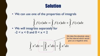
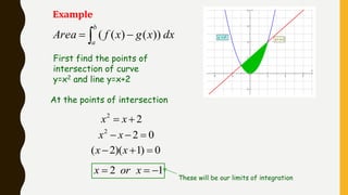
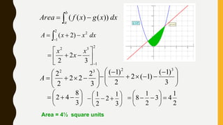
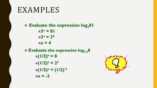
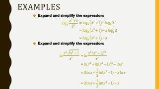
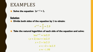
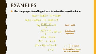
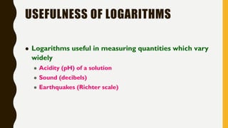
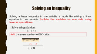
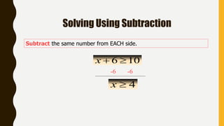
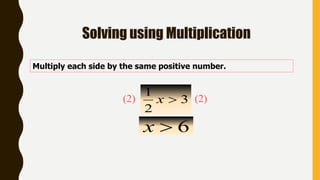
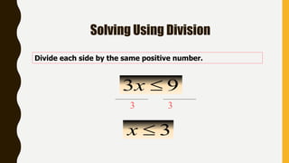
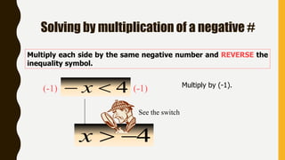
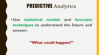
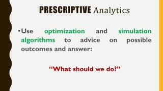
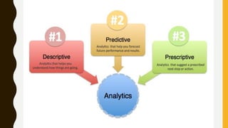
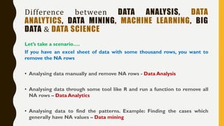
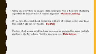
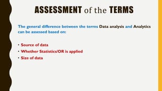
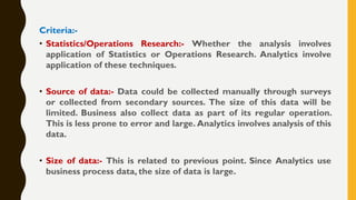
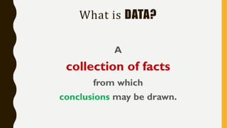
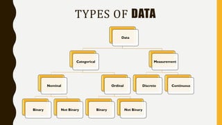
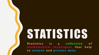
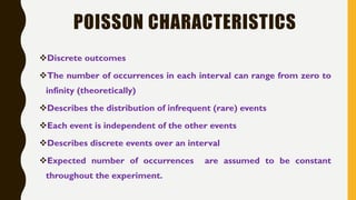
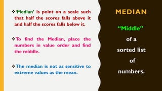
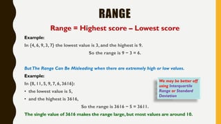
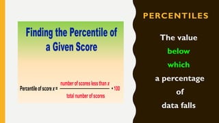
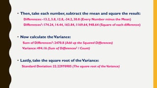
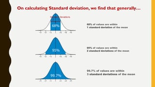
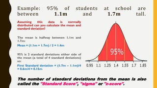
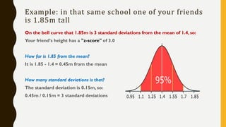
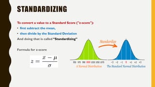
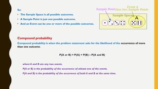
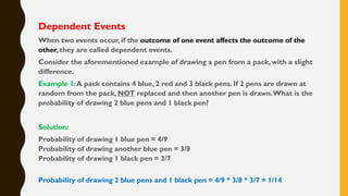
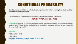
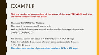
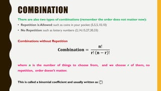
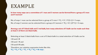
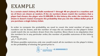
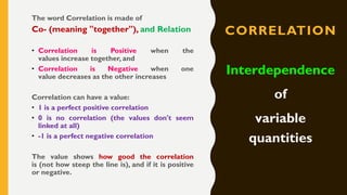
Analytics is the process of examining data to draw conclusions and inform decision making. It involves descriptive, predictive, and prescriptive models. Descriptive models analyze past data to understand what has occurred, predictive models use statistical techniques to forecast future outcomes, and prescriptive models advise on potential actions and outcomes. Common techniques in analytics include statistics, machine learning, and visualization of large datasets.


![SOLUTION
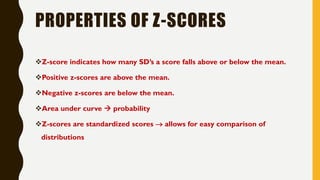
• Note:What is meant here by area is the area under the standard normal curve.
a) For x = 40, the z-value z = (40 - 30) / 4 = 2.5
Hence P(x < 40) = P(z < 2.5) = [area to the left of 2.5] = 0.9938
b) For x = 21, z = (21 - 30) / 4 = -2.25
Hence P(x > 21) = P(z > -2.25) = [total area] - [area to the left of -2.25]
= 1 - 0.0122 = 0.9878
c) For x = 30 , z = (30 - 30) / 4 = 0 and for x = 35, z = (35 - 30) / 4 = 1.25
Hence P(30 < x < 35) = P(0 < z < 1.25) = [area to the left of z = 1.25] - [area to the left
of 0]
= 0.8944 - 0.5 = 0.3944](https://image.slidesharecdn.com/statisticsforanalytics-181001113510/85/Statistics-for-analytics-29-320.jpg)
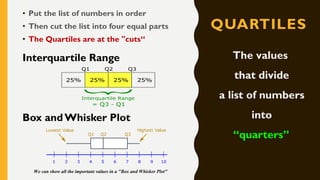
![SOLUTION
• Let x be the random variable that represents the speed of cars. x has μ = 90 and σ
= 10.We have to find the probability that x is higher than 100 or P(x > 100)
For x = 100 , z = (100 - 90) / 10 = 1
P(x > 90) = P(z >, 1) = [total area] - [area to the left of z = 1]
= 1 - 0.8413 = 0.1587
The probability that a car selected at a random has a speed greater than 100
km/hr is equal to 0.1587](https://image.slidesharecdn.com/statisticsforanalytics-181001113510/85/Statistics-for-analytics-31-320.jpg)
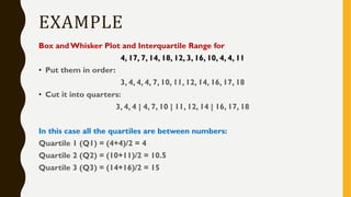
![SOLUTION
• Let x be the random variable that represents the length of time. It has a mean of 50
and a standard deviation of 15.We have to find the probability that x is between 50 and
70 or P( 50< x < 70)
For x = 50 , z = (50 - 50) / 15 = 0
For x = 70 , z = (70 - 50) / 15 = 1.33 (rounded to 2 decimal places)
P( 50< x < 70) = P( 0< z < 1.33) = [area to the left of z = 1.33] - [area to the left of z =
0]
= 0.9082 - 0.5 = 0.4082
The probability that John's computer has a length of time between 50 and 70 hours is
equal to 0.4082.](https://image.slidesharecdn.com/statisticsforanalytics-181001113510/85/Statistics-for-analytics-33-320.jpg)
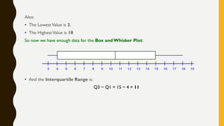


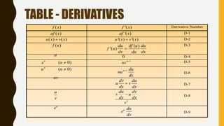
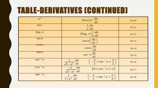
![THE POWER RULE
1
[ ] , is any real numberN Nd
x Nx N
dx
[ ] 1
d
x
dx
](https://image.slidesharecdn.com/statisticsforanalytics-181001113510/85/Statistics-for-analytics-92-320.jpg)
![THE CONSTANT RULE
[ ] 0, is a constant
d
c c
dx
The derivative of a constant function is zero.](https://image.slidesharecdn.com/statisticsforanalytics-181001113510/85/Statistics-for-analytics-93-320.jpg)
![THE CONSTANT MULTIPLE RULE
[ ( ) ] '( ) , is a constant
d
c f x c f x c
dx
The derivative of a constant times a function is equal to the constant
times the derivative of the function.](https://image.slidesharecdn.com/statisticsforanalytics-181001113510/85/Statistics-for-analytics-94-320.jpg)
![THE SUM AND DIFFERENCE RULES
[ ( ) ( )] '( ) '( )
d
f x g x f x g x
dx
The derivative of a sum is the sum of the derivatives.
[ ( ) ( )] '( ) '( )
d
f x g x f x g x
dx
The derivative of a difference is the difference of the derivatives.](https://image.slidesharecdn.com/statisticsforanalytics-181001113510/85/Statistics-for-analytics-95-320.jpg)