Probabilit
y
Probability is ameasure of how
often a particular event will
happen if something is done
repeatedly. It is a chance that
something will happen.
4.
●There is a20 percent
chance of rain tomorrow.
●The probability of winning
the lottery is one in many
millions.
Examples:
5.
Suppose three coinsare
tossed. Let Y be the random
variable representing the number
of tails that occur. Find the
probability of each of the values of
the random variable Y.
Example 1:
6.
Solution:
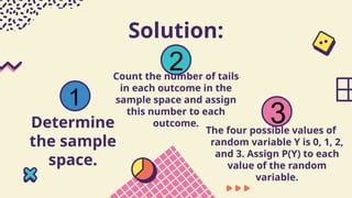
Determine
the sample
space.
Count thenumber of tails
in each outcome in the
sample space and assign
this number to each
outcome.
The four possible values of
random variable Y is 0, 1, 2,
and 3. Assign P(Y) to each
value of the random
variable.
1
2
3
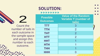
Count the
number oftails in
each outcome in
the sample space
and assign this
number to each
outcome.
SOLUTION:
Possible
Outcomes
Value of the Random
Variable Y (number of
tails)
TTT 3
TTH 2
THT 2
HTT 2
HHT 1
HTH 1
THH 1
HHH 0
9.
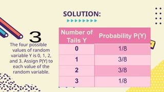
The four possible
valuesof random
variable Y is 0, 1, 2,
and 3. Assign P(Y) to
each value of the
random variable.
SOLUTION:
Number of
Tails Y
Probability P(Y)
0 1/8
1 3/8
2 3/8
3 1/8
10.
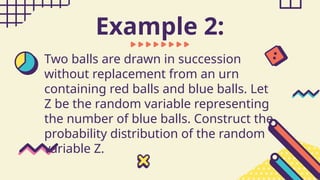
Two balls aredrawn in succession
without replacement from an urn
containing red balls and blue balls. Let
Z be the random variable representing
the number of blue balls. Construct the
probability distribution of the random
variable Z.
Example 2:
11.
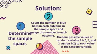
Solution:
Determine
the sample
space.
Count thenumber of blue
balls in each outcome in
the sample space and
assign this number to each
outcome.
The four possible values of
random variable Z is 0, 1, and
2. Assign P(Z) to each value
of the random variable.
1
2
3
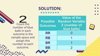
Count the
number ofblue
balls in each
outcome in the
sample space and
assign this
number to each
outcome.
SOLUTION:
Possible
Outcomes
Value of the
Random Variable
Z (number of
blue balls)
RR 0
RB 1
BR 1
BB 2
14.
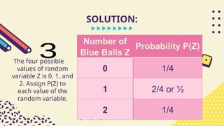
The four possible
valuesof random
variable Z is 0, 1, and
2. Assign P(Z) to
each value of the
random variable.
SOLUTION:
Number of
Blue Balls Z
Probability P(Z)
0 1/4
1 2/4 or ½
2 1/4
15.
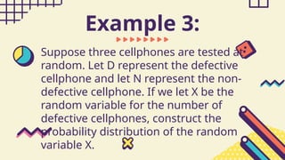
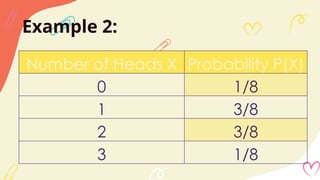
Suppose three cellphonesare tested at
random. Let D represent the defective
cellphone and let N represent the non-
defective cellphone. If we let X be the
random variable for the number of
defective cellphones, construct the
probability distribution of the random
variable X.
Example 3:
16.
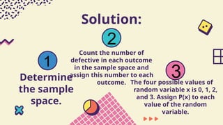
Solution:
Determine
the sample
space.
Count thenumber of
defective in each outcome
in the sample space and
assign this number to each
outcome. The four possible values of
random variable x is 0, 1, 2,
and 3. Assign P(x) to each
value of the random
variable.
1
2
3
Count the
number of
defectivein each
outcome in the
sample space and
assign this
number to each
outcome.
SOLUTION:
Possible Outcomes
Value of the Random
Variable X (number of
defective cellphones)
NNN 0
NND 1
NDN 1
DNN 1
NDD 2
DND 2
DDN 2
DDD 3
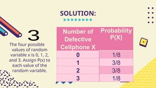
19.
The four possible
valuesof random
variable x is 0, 1, 2,
and 3. Assign P(x) to
each value of the
random variable.
SOLUTION:
Number of
Defective
Cellphone X
Probability
P(X)
0 1/8
1 3/8
2 3/8
3 1/8
20.
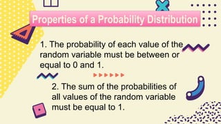
Properties of aProbability Distribution
2. The sum of the probabilities of
all values of the random variable
must be equal to 1.
1. The probability of each value of the
random variable must be between or
equal to 0 and 1.
Mean
Mean is simplythe average that we are
familiar to, where you add all the
numbers and divide it by the total
number of the numbers you added.
23.
Consider rolling adie.
What is the average
number of spots that would
appear?
Example 1:
24.
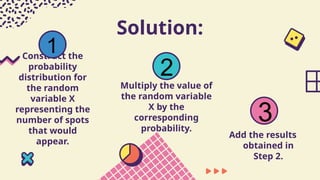
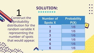
Solution:
Construct the
probability
distribution for
therandom
variable X
representing the
number of spots
that would
appear.
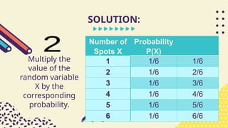
Multiply the value of
the random variable
X by the
corresponding
probability.
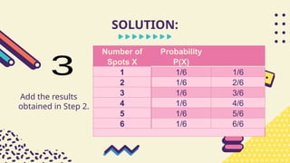
Add the results
obtained in
Step 2.
1
2
3
Multiply the
value ofthe
random variable
X by the
corresponding
probability.
SOLUTION:
Number of
Spots X
Probability
P(X)
1 1/6 1/6
2 1/6 2/6
3 1/6 3/6
4 1/6 4/6
5 1/6 5/6
6 1/6 6/6
27.
Add the results
obtainedin Step 2.
SOLUTION:
Number of
Spots X
Probability
P(X)
1 1/6 1/6
2 1/6 2/6
3 1/6 3/6
4 1/6 4/6
5 1/6 5/6
6 1/6 6/6
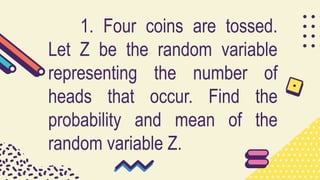
1. Four coinsare tossed.
Let Z be the random variable
representing the number of
heads that occur. Find the
probability and mean of the
random variable Z.
30.
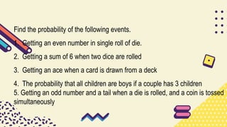
Find the probabilityof the following events.
1. Getting an even number in single roll of die.
2. Getting a sum of 6 when two dice are rolled
3. Getting an ace when a card is drawn from a deck
4. The probability that all children are boys if a couple has 3 children
5. Getting an odd number and a tail when a die is rolled, and a coin is tossed
simultaneously
31.
9th Grade
Computing theVariance
and Standard Deviation
of a Discrete
Probability
Distribution
32.
RECAP
01
VARIANCE OF ADISCRETE
PROBABILITY
DISTIRBUTION
ASSIGNMENT
03 ACTIVITY
04
02
LESSON 3
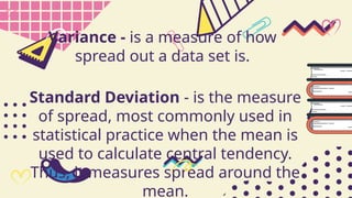
Standard Deviation -is the measure
of spread, most commonly used in
statistical practice when the mean is
used to calculate central tendency.
Thus, it measures spread around the
mean.
Variance - is a measure of how
spread out a data set is.
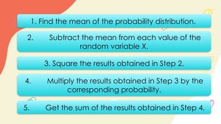
1. Find themean of the probability distribution.
2. Subtract the mean from each value of the
random variable X.
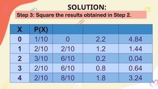
3. Square the results obtained in Step 2.
5. Get the sum of the results obtained in Step 4.
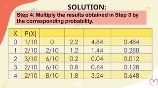
4. Multiply the results obtained in Step 3 by the
corresponding probability.
38.
Example 1: Numberof Cars
Sold
The number of cars sold per day at
a local car dealership, along with its
corresponding probabilities, is shown in
the succeeding table. Compute the
variance and the standard deviation of
the probability distribution by following
the given steps.
39.
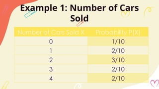
Example 1: Numberof Cars
Sold
Number of Cars Sold X Probability P(X)
0 1/10
1 2/10
2 3/10
3 2/10
4 2/10
40.
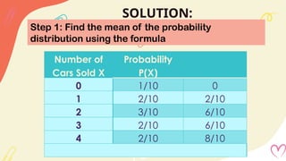
SOLUTION:
Step 1: Findthe mean of the probability
distribution using the formula
Number of
Cars Sold X
Probability
P(X)
0 1/10 0
1 2/10 2/10
2 3/10 6/10
3 2/10 6/10
4 2/10 8/10
41.
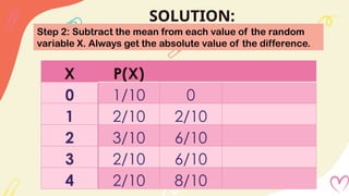
SOLUTION:
Step 2: Subtractthe mean from each value of the random
variable X. Always get the absolute value of the difference.
X P(X)
0 1/10 0
1 2/10 2/10
2 3/10 6/10
3 2/10 6/10
4 2/10 8/10
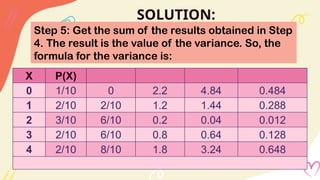
SOLUTION:
Step 5: Getthe sum of the results obtained in Step
4. The result is the value of the variance. So, the
formula for the variance is:
𝜎
2
=∑(𝑋−𝜇)2
∙𝑃(𝑋)
45.
SOLUTION:
Step 5: Getthe sum of the results obtained in Step
4. The result is the value of the variance. So, the
formula for the variance is:
X P(X)
0 1/10 0 2.2 4.84 0.484
1 2/10 2/10 1.2 1.44 0.288
2 3/10 6/10 0.2 0.04 0.012
3 2/10 6/10 0.8 0.64 0.128
4 2/10 8/10 1.8 3.24 0.648
46.
SOLUTION:
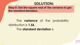
Step 6: Getthe square root of the variance to get
the standard deviation.
The variance of the probability
distribution is 1.56.
The standard deviation is
47.
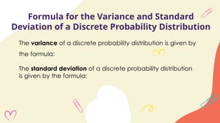
Formula for theVariance and Standard
Deviation of a Discrete Probability Distribution
The variance of a discrete probability distribution is given by
the formula:
The standard deviation of a discrete probability distribution
is given by the formula:
48.
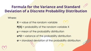
Formula for theVariance and Standard
Deviation of a Discrete Probability Distribution
Where:
X = value of the random variable
P(X) = probability of the random variable X
μ = mean of the probability distribution
σ^2 = variance of the probability distribution
σ = standard deviation of the probability distribution
49.
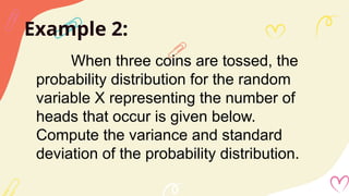
Example 2:
When threecoins are tossed, the
probability distribution for the random
variable X representing the number of
heads that occur is given below.
Compute the variance and standard
deviation of the probability distribution.
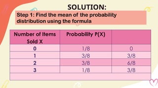
SOLUTION:
Step 1: Findthe mean of the probability
distribution using the formula
Number of Items
Sold X
Probability P(X)
0 1/8 0
1 3/8 3/8
2 3/8 6/8
3 1/8 3/8
52.
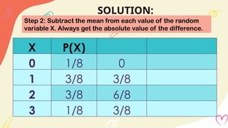
SOLUTION:
Step 2: Subtractthe mean from each value of the random
variable X. Always get the absolute value of the difference.
X P(X)
0 1/8 0
1 3/8 3/8
2 3/8 6/8
3 1/8 3/8
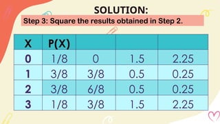
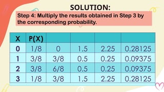
SOLUTION:
Step 4: Multiplythe results obtained in Step 3 by
the corresponding probability.
X P(X)
0 1/8 0 1.5 2.25 0.28125
1 3/8 3/8 0.5 0.25 0.09375
2 3/8 6/8 0.5 0.25 0.09375
3 1/8 3/8 1.5 2.25 0.28125
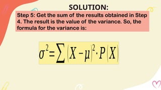
55.
SOLUTION:
Step 5: Getthe sum of the results obtained in Step
4. The result is the value of the variance. So, the
formula for the variance is:
𝜎
2
=∑(𝑋−𝜇)2
∙𝑃(𝑋)
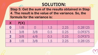
56.
SOLUTION:
Step 5: Getthe sum of the results obtained in Step
4. The result is the value of the variance. So, the
formula for the variance is:
X P(X)
0 1/8 0 1.5 2.25 0.28125
1 3/8 3/8 0.5 0.25 0.09375
2 3/8 6/8 0.5 0.25 0.09375
3 1/8 3/8 1.5 2.25 0.28125
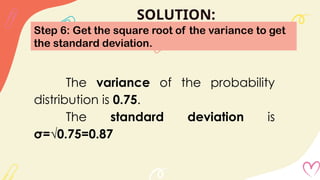
57.
SOLUTION:
Step 6: Getthe square root of the variance to get
the standard deviation.
The variance of the probability
distribution is 0.75.
The standard deviation is
σ=√0.75=0.87
58.
Example 3:
The numberof items sold per day
at a retail store with its corresponding
probabilities, is shown in the table. Find
the variance and standard deviation of
the probability distribution.
59.
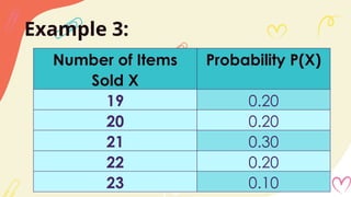
Example 3:
Number ofItems
Sold X
Probability P(X)
19 0.20
20 0.20
21 0.30
22 0.20
23 0.10
60.
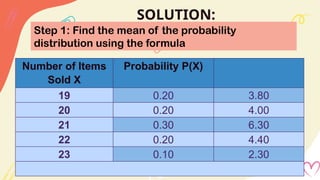
SOLUTION:
Step 1: Findthe mean of the probability
distribution using the formula
Number of Items
Sold X
Probability P(X)
19 0.20 3.80
20 0.20 4.00
21 0.30 6.30
22 0.20 4.40
23 0.10 2.30
61.
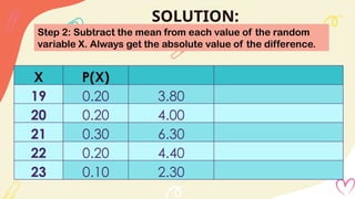
SOLUTION:
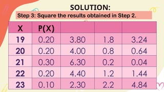
Step 2: Subtractthe mean from each value of the random
variable X. Always get the absolute value of the difference.
X P(X)
19 0.20 3.80
20 0.20 4.00
21 0.30 6.30
22 0.20 4.40
23 0.10 2.30
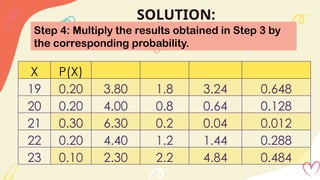
SOLUTION:
Step 5: Getthe sum of the results obtained in Step
4. The result is the value of the variance. So, the
formula for the variance is:
𝜎
2
=∑(𝑋−𝜇)2
∙𝑃(𝑋)
65.
SOLUTION:
Step 5: Getthe sum of the results obtained in Step
4. The result is the value of the variance. So, the
formula for the variance is:
X P(X)
19 0.20 3.80 1.8 3.24 0.648
20 0.20 4.00 0.8 0.64 0.128
21 0.30 6.30 0.2 0.04 0.012
22 0.20 4.40 1.2 1.44 0.288
23 0.10 2.30 2.2 4.84 0.484
66.
SOLUTION:
Step 6: Getthe square root of the variance to get
the standard deviation.
The variance of the probability
distribution is 1.56.
The standard deviation is
σ=√1.56=1.25
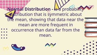
Normal Distribution -is a probability
distribution that is symmetric about
the mean, showing that data near the
mean are more frequent in
occurrence than data far from the
mean.
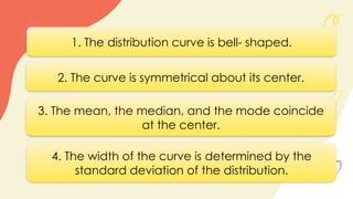
1. The distributioncurve is bell- shaped.
2. The curve is symmetrical about its center.
3. The mean, the median, and the mode coincide
at the center.
4. The width of the curve is determined by the
standard deviation of the distribution.
71.
5. The tailsof the curve flatten out indefinitely along
the horizontal axis, always approaching the axis but
never touching it. That is, the curve is asymptotic to
the base line.
6. The area under the curve is 1. Thus, it
represents the probability or proportion, or the
percentage associated with specific sets of
measurement values.
72.
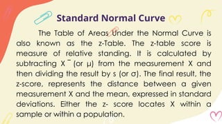
Standard Normal Curve
Thestandard normal curve is a normal
probability distribution that is most commonly used as
a model for inferential statistics. The equation the
describes a normal curve is:
73.
Standard Normal Curve
Where:Y = height of the curve particular values of X
X = any score in the distribution
σ = standard deviation of the population
μ = mean of the population
π = 3.1416
e = 2.7183
74.
Standard Normal Curve
Astandard normal curve is a normal probability
distribution that has a mean of 0 and a standard
deviation of 1.
75.
Standard Normal Curve
TheTable of Areas Under the Normal Curve is
also known as the z-Table. The z-table score is
measure of relative standing. It is calculated by
subtracting X (or μ) from the measurement X and
̅
then dividing the result by s (or σ). The final result, the
z-score, represents the distance between a given
measurement X and the mean, expressed in standard
deviations. Either the z- score locates X within a
sample or within a population.
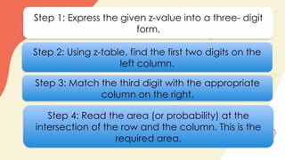
Step 1: Expressthe given z-value into a three- digit
form.
Step 2: Using z-table, find the first two digits on the
left column.
Step 3: Match the third digit with the appropriate
column on the right.
Step 4: Read the area (or probability) at the
intersection of the row and the column. This is the
required area.
78.
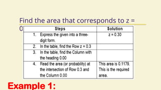
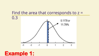
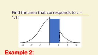
Example 1:
1. Findthe area that corresponds to z = 1.
Finding the area that corresponds to is
the same as finding the area between z
= 0 and z = 1.
79.
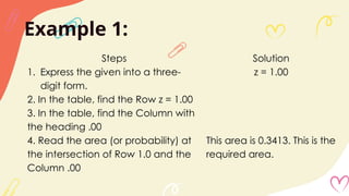
Example 1:
Steps Solution
1.Express the given into a three-
digit form.
z = 1.00
2. In the table, find the Row z = 1.00
3. In the table, find the Column with
the heading .00
4. Read the area (or probability) at
the intersection of Row 1.0 and the
Column .00
This area is 0.3413. This is the
required area.
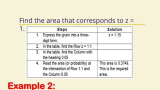
80.
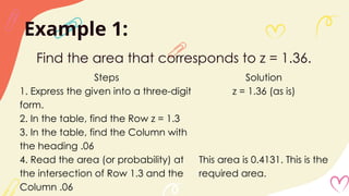
Example 1:
Steps Solution
1.Express the given into a three-digit
form.
z = 1.36 (as is)
2. In the table, find the Row z = 1.3
3. In the table, find the Column with
the heading .06
4. Read the area (or probability) at
the intersection of Row 1.3 and the
Column .06
This area is 0.4131. This is the
required area.
Find the area that corresponds to z = 1.36.
CREDITS: This presentationtemplate was created by Slidesgo,
including icons by Flaticon, infographics & images by Freepik and
illustrations by Storyset
THANKS!
Please keep this slide for attribution
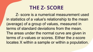
THE Z- SCORE
Z-score is a numerical measurement used
in statistics of a value's relationship to the mean
(average) of a group of values, measured in
terms of standard deviations from the mean.
The areas under the normal curve are given in
terms of z-values or scores. Either the z-score
locates X within a sample or within a population.
85.
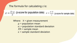
The formula forcalculating z is:
Where: X = given measurement
𝜇 = population mean
𝜎 = population standard deviation
𝑋̅X = sample mean
𝑠 = sample standard deviation
86.
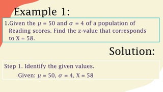
Example 1:
1.Given the𝜇 = 50 and 𝜎 = 4 of a population of
Reading scores. Find the z-value that corresponds
to X = 58.
Solution:
Step 1. Identify the given values.
Given: = 50, = 4, X = 58
𝜇 𝜎
87.
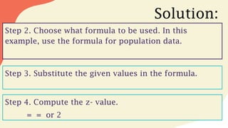
Solution:
Step 2. Choosewhat formula to be used. In this
example, use the formula for population data.
Step 3. Substitute the given values in the formula.
Step 4. Compute the z- value.
= = or 2
88.
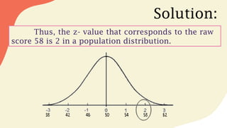
Solution:
Thus, the z-value that corresponds to the raw
score 58 is 2 in a population distribution.
89.
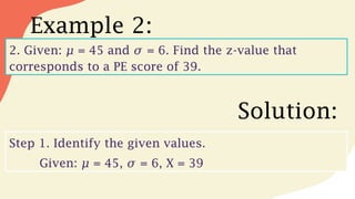
Example 2:
2. Given:= 45 and = 6. Find the z-value that
𝜇 𝜎
corresponds to a PE score of 39.
Solution:
Step 1. Identify the given values.
Given: = 45, = 6, X = 39
𝜇 𝜎
90.
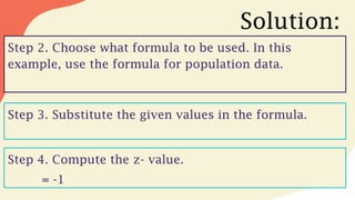
Solution:
Step 2. Choosewhat formula to be used. In this
example, use the formula for population data.
Step 3. Substitute the given values in the formula.
Step 4. Compute the z- value.
= -1
91.
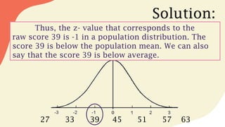
Solution:
Thus, the z-value that corresponds to the
raw score 39 is -1 in a population distribution. The
score 39 is below the population mean. We can also
say that the score 39 is below average.
27 33 39 45 51 57 63
92.
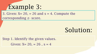
Example 3:
3. Given:X= 20, = 26 and s = 4. Compute the
corresponding z- score.
Solution:
Step 1. Identify the given values.
Given: X= 20, = 26 , s = 4
93.
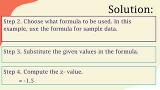
Solution:
Step 2. Choosewhat formula to be used. In this
example, use the formula for sample data.
Step 3. Substitute the given values in the formula.
Step 4. Compute the z- value.
= -1.5
94.
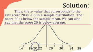
Solution:
Thus, the z-value that corresponds to the
raw score 20 is -1.5 in a sample distribution. The
score 20 is below the sample mean. We can also
say that the score 20 is below average.
14 18 20 22 26 30 34 38
95.
ACTIVITY :2
State whetherthe z- score locates the raw score
within a sample or within a population. Write S for
sample and P for population.
1. - ________________
2. - ________________
3. - ________________
4. - _______________
5. - ______________
96.
QUIZ 2:
Find thez- score value that corresponds to
each of the following scores up to two decimal
places.
Given:
1. X=70
2. X=50
3. X=42
4. X=78
5. X=82
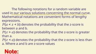
Note:
When z isnegative, we simply ignore the
negative sign and proceed as before. The
negative sign informs us that the region we
are interested in is found on the left side of
the mean. Areas are positive values.
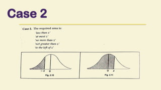
Note:
The following notationsfor a random variable are
used in our various solutions concerning the normal curve.
Mathematical notations are convenient forms of lengthy
expressions.
𝑃( < < )
𝑎 𝑧 𝑏 denotes the probability that the z-score is
between a and b.
𝑃( > )
𝑧 𝑎 denotes the probability that the z-score is greater
than a.
𝑃( < )
𝑧 𝑎 denotes the probability that the z-score is less than
a. Where a and b are z-score values
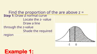
Example 1:
Find theproportion of the are above z =
-1.
Step 1: Draw a normal curve
Locate the z- value
Draw a line
through the z-value
Shade the required
region
108.
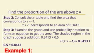
Example 1:
Find theproportion of the are above z =
-1.
Step 2: Consult the z- table and find the area that
corresponds to z = -1.
z = -1 corresponds to an area of 0.3413
Step 3: Examine the graph and use probability notation to
form an equation to get the area. The shaded region in the
graph suggests addition. 0.3413 + 0.5
𝑃( > 1) = 0.3413 +
𝑧 −
0.5 = 0.8413
109.
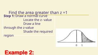
Example 2:
Find thearea greater than z =1
Step 1: Draw a normal curve
Locate the z- value
Draw a line
through the z-value
Shade the required
region
110.
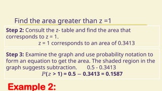
Example 2:
Find thearea greater than z =1
Step 2: Consult the z- table and find the area that
corresponds to z = 1.
z = 1 corresponds to an area of 0.3413
Step 3: Examine the graph and use probability notation to
form an equation to get the area. The shaded region in the
graph suggests subtraction. 0.5 - 0.3413
𝑃( > 1) = 0.5 0.3413 = 0.1587
𝑧 −
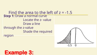
Example 3:
Find thearea to the left of z = -1.5
Step 1: Draw a normal curve
Locate the z- value
Draw a line
through the z-value
Shade the required
region
113.
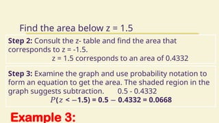
Example 3:
Find thearea below z = 1.5
Step 2: Consult the z- table and find the area that
corresponds to z = -1.5.
z = 1.5 corresponds to an area of 0.4332
Step 3: Examine the graph and use probability notation to
form an equation to get the area. The shaded region in the
graph suggests subtraction. 0.5 - 0.4332
𝑃( < 1.5) = 0.5 0.4332 = 0.0668
𝑧 − −
114.
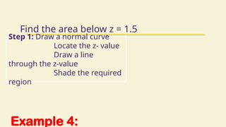
Example 4:
Find thearea below z = 1.5
Step 1: Draw a normal curve
Locate the z- value
Draw a line
through the z-value
Shade the required
region
115.
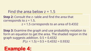
Example 4:
Find thearea below z = 1.5
Step 2: Consult the z- table and find the area that
corresponds to z = 1.5.
z = 1.5 corresponds to an area of 0.4332
Step 3: Examine the graph and use probability notation to
form an equation to get the area. The shaded region in the
graph suggests addition. 0.5 + 0.4332
𝑃( < 1.5) = 0.5 + 0.4332 = 0.9332
𝑧
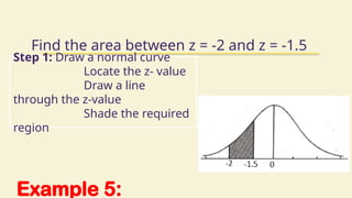
Example 5:
Find thearea between z = -2 and z = -1.5
Step 1: Draw a normal curve
Locate the z- value
Draw a line
through the z-value
Shade the required
region
118.
Example 5:
Find thearea between z = -2 and z = -1.5
Step 2: Consult the z- table and find the area that
corresponds to z = -2 and z = -1.5.
z = -2 corresponds to 0.4772 z = -1.5
corresponds to 0.4332
Step 3: Examine the graph and use probability notation to
form an equation to get the area. The shaded region in the
graph suggests subtraction. 0.4772 - 0.4332
𝑃( 2 < < 1.5) = 0.4772 0.4332 = 0.0440
− 𝑧 − −
119.
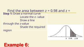
Example 6:
Find thearea between z = 0.98 and z =
2.58
Step 1: Draw a normal curve
Locate the z- value
Draw a line
through the z-value
Shade the required
region
120.
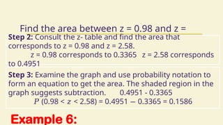
Example 6:
Find thearea between z = 0.98 and z =
2.58
Step 2: Consult the z- table and find the area that
corresponds to z = 0.98 and z = 2.58.
z = 0.98 corresponds to 0.3365 z = 2.58 corresponds
to 0.4951
Step 3: Examine the graph and use probability notation to
form an equation to get the area. The shaded region in the
graph suggests subtraction. 0.4951 - 0.3365
𝑃 (0.98 < < 2.58) = 0.4951 0.3365 = 0.1586
𝑧 −
Sampling is theprocess of
selecting observations (a sample)
to provide an adequate
description and inferences of the
population.
It means selecting the group
that you will actually collect data
from in your research.
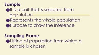
Sample
●It is aunit that is selected from
population
●Represents the whole population
●Purpose to draw the inference
Sampling Frame
●Listing of population from which a
sample is chosen
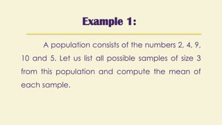
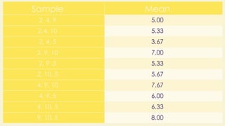
Example 1:
A populationconsists of the numbers 2, 4, 9,
10 and 5. Let us list all possible samples of size 3
from this population and compute the mean of
each sample.
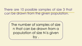
There are 10possible samples of size 3 that
can be drawn from the given population.
The number of samples of size
n that can be drawn from a
population of size N is given
by .
131.
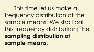
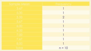
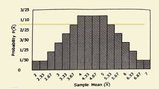
This time letus make a
frequency distribution of the
sample means. We shall call
this frequency distribution; the
sampling distribution of
sample means.
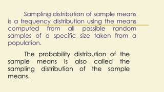
Sampling distribution ofsample means
is a frequency distribution using the means
computed from all possible random
samples of a specific size taken from a
population.
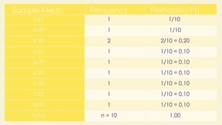
The probability distribution of the
sample means is also called the
sampling distribution of the sample
means.
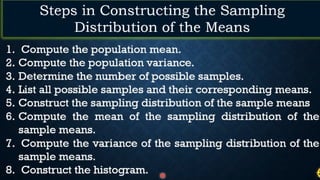
1. Determine thenumber of
possible samples that can be
drawn from the population using
the formula:
Where N = size of the
population
n = size of the sample
138.
2. List allthe possible samples
and compute the mean of each
sample.
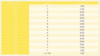
3. Construct a frequency
distribution of the sample means
obtained in Step 2.
139.
Example 2:
Samples ofthree cards are
drawn at random from a
population of eight cards
numbered from 1 to 8.
140.
Example 2:
a. Howmany possible
samples can be drawn?
Given: N = 8 and n = 3.
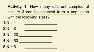
Activity 1: Howmany different samples of
size r= 3 can be selected from a population
with the following sizes?
1.N = 4 ______nCr = 4C3 = 4_________
2.N = 8 ______ nCr = 56_________
3.N = 20 _____ nCr = 1140__________
4.N = 50 _____ nCr = 19600__________
5.N = 6 ______ nCr = 20_________
147.
Activity 1: Howmany different samples of
size r= 3 can be selected from a population
with the following sizes?
1.N = 4 _______________
2.N = 8 _______________
3.N = 20 _______________
4.N = 50 _______________
5.N = 6 _______________
148.
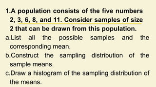
1.A population consistsof the five numbers
2, 3, 6, 8, and 11. Consider samples of size
2 that can be drawn from this population.
a.List all the possible samples and the
corresponding mean.
b.Construct the sampling distribution of the
sample means.
c.Draw a histogram of the sampling distribution of
the means.
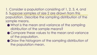
1. Consider apopulation consisting of 1, 2, 3, 4, and
5. Suppose samples of size 2 are drawn from this
population. Describe the sampling distribution of the
sample means.
● What is the mean and variance of the sampling
distribution of the sample means?
● Compare these values to the mean and variance
of the population.
● Draw the histogram of the sampling distribution of
the population mean.
154.
Compute the meanof the
population .
So, the mean of the population is
3.00.
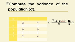
Compute the varianceof the
population (σ).
X
1 2 4
2 1 1
3 0 0
4 1 1
5 2 4
𝜎2
=
∑(𝑿 −𝝁¿¿¿¿2
𝑁
=
𝟏𝟎
𝟓
=𝟐
157.
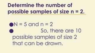
Determine the numberof
possible samples of size n = 2.
●N = 5 and n = 2
● So, there are 10
possible samples of size 2
that can be drawn.
158.
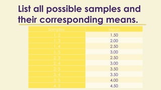
List all possiblesamples and
their corresponding means.
Samples Mean
1, 2 1.50
1, 3 2.00
1, 4 2.50
1, 5 3.00
2, 3 2.50
2, 4 3.00
2, 5 3.50
3, 4 3.50
3, 5 4.00
4, 5 4.50
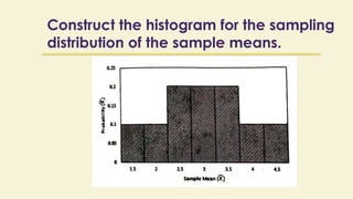
159.
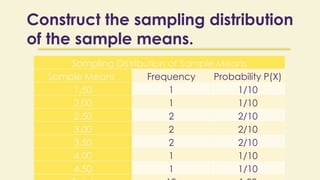
Construct the samplingdistribution
of the sample means.
Sampling Distribution of Sample Means
Sample Means Frequency Probability P(X)
1.50 1 1/10
2.00 1 1/10
2.50 2 2/10
3.00 2 2/10
3.50 2 2/10
4.00 1 1/10
4.50 1 1/10
160.
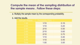
Compute the meanof the sampling distribution of
the sample means . Follow these steps:
a. Multiply the sample mean by the corresponding probability.
b. Add the results.
Sample Means Probability P(X)
1.50 1/10 0.15
2.00 1/10 0.20
2.50 2/10 0.50
3.00 2/10 0.60
3.50 2/10 0.70
4.00 1/10 0.40
4.50 1/10 0.45
Total 1.00 3.00
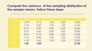
161.
Compute the varianceof the sampling distribution
of the sample means. Follow these steps:
• Subtract the population mean from each
sample mean . Do not forget to use the
absolute value function in each difference.
Label this as ||.
• Square the difference. Label this as .
• Multiply the results by the corresponding
probability. Label this as .
• Add the results.
162.
Compute the varianceof the sampling distribution of
the sample means. Follow these steps:
X P(X) ||
1.50 1/10 0.15 1.50 2.25 0.225
2.00 1/10 0.20 1.00 1.00 0.100
2.50 2/10 0.50 0.50 0.25 0.050
3.00 2/10 0.60 0.00 0.00 0.000
3.50 2/10 0.70 0.50 0.25 0.050
4.00 1/10 0.40 1.00 1.00 0.100
4.50 1/10 0.45 1.50 2.25 0.225
Total 1.00 3.00 0.750
163.
Compute the varianceof the sampling distribution
of the sample means. Follow these steps:
So, the variance of the
sampling distribution is 0.75.
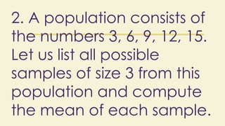
2. A populationconsists of
the numbers 3, 6, 9, 12, 15.
Let us list all possible
samples of size 3 from this
population and compute
the mean of each sample.
T-DISTRIBUTION
oAlso called Student’st-distribution
is a family of distributions that look
almost identical to the normal
distribution curve, only a bit shorter
and stouter.
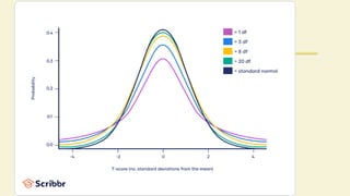
T-DISTRIBUTION
o The t-distributionis used instead of the
normal distribution when you have small
samples. The larger the sample size, the
more the t distribution looks like the normal
distribution. In fact, for sample sizes larger
than 20, the distribution is almost exactly like
the normal distribution.
171.
T-DISTRIBUTION
o Like thenormal distribution, the t-
distribution has a smooth shape.
o Like the normal distribution, the t-
distribution is symmetric. If you think about
folding it in half at the mean, each side will
be the same.
172.
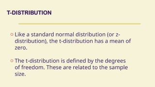
T-DISTRIBUTION
o Like astandard normal distribution (or z-
distribution), the t-distribution has a mean of
zero.
o The t-distribution is defined by the degrees
of freedom. These are related to the sample
size.
173.
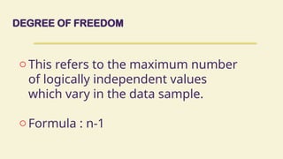
DEGREE OF FREEDOM
oThis refers to the maximum number
of logically independent values
which vary in the data sample.
o Formula : n-1
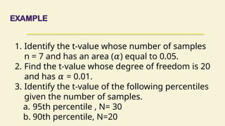
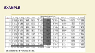
EXAMPLE
1. Identify thet-value whose number of samples
n = 7 and has an area ( ) equal to 0.05.
𝛼
2. Find the t-value whose degree of freedom is 20
and has = 0.01.
𝛼
3. Identify the t-value of the following percentiles
given the number of samples.
a. 95th percentile , N= 30
b. 90th percentile, N=20
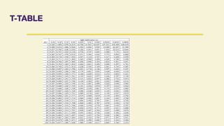
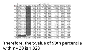
177.
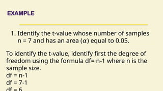
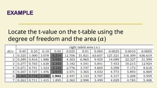
EXAMPLE
1. Identify thet-value whose number of samples
n = 7 and has an area ( ) equal to 0.05.
𝛼
To identify the t-value, identify first the degree of
freedom using the formula df= n-1 where n is the
sample size.
df = n-1
df = 7-1
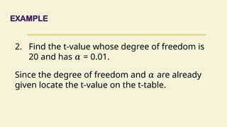
EXAMPLE
2. Find thet-value whose degree of freedom is
20 and has = 0.01.
𝛼
Since the degree of freedom and are already
𝛼
given locate the t-value on the t-table.
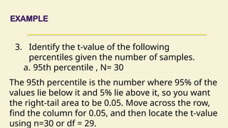
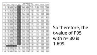
EXAMPLE
3. Identify thet-value of the following
percentiles given the number of samples.
a. 95th percentile , N= 30
The 95th percentile is the number where 95% of the
values lie below it and 5% lie above it, so you want
the right-tail area to be 0.05. Move across the row,
find the column for 0.05, and then locate the t-value
using n=30 or df = 29.
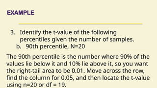
EXAMPLE
3. Identify thet-value of the following
percentiles given the number of samples.
b. 90th percentile, N=20
The 90th percentile is the number where 90% of the
values lie below it and 10% lie above it, so you want
the right-tail area to be 0.01. Move across the row,
find the column for 0.05, and then locate the t-value
using n=20 or df = 19.
CONFIDENCE INTERVAL
An intervalestimate, called a confidence interval, is a
range of values or interval (with lower and upper limits)
used to estimate the population parameter. This estimate
may or may not contain the true parameter value. The
parameter is specified as being between two values. It is
usually in the form of a < ϴ < b, which tells that the
estimated parameter (ϴ) is between two values (a and b)
at a certain level of confidence.)
187.
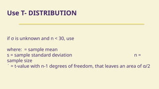
Use T- DISTRIBUTION
ifσ is unknown and n < 30, use
where: = sample mean
s = sample standard deviation n =
sample size
̇ = t-value with n-1 degrees of freedom, that leaves an area of α/2
188.
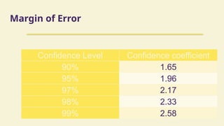
Margin of Error
iscalled margin of error. However, when σ
is not known (as is often the case), the
sample standard deviation s is used to
approximate σ. So, the formula for E is
modified.
189.
Example 1:
Compute themargin of error of the 90% confidence
interval estimate of µ when s = 5, n = 16.
Given: s= 5
n= 16
confidence level = 90%
190.
Example 1:
Compute themargin of error of the 90% confidence
interval estimate of µ when s = 5, n = 16.
Formula:
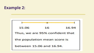
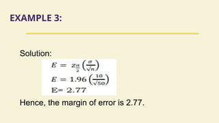
Example 2:
The averagehemoglobin reading for a sample of 20
teachers was 16 grams per 100 milliliters with a sample
standard deviation of 2 grams. Find the 95% confidence
interval of the true mean.
Given: Confidence Level = 95%
n= 20 s = 2
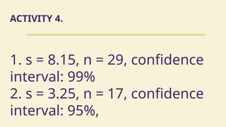
ACTIVITY 4.
1. s= 8.15, n = 29, confidence
interval: 99%
2. s = 3.25, n = 17, confidence
interval: 95%,
199.
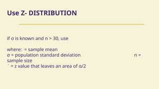
Use Z- DISTRIBUTION
ifσ is known and n > 30, use
where: = sample mean
σ = population standard deviation n =
sample size
̇ = z value that leaves an area of α/2
200.
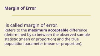
Margin of Error
iscalled margin of error.
Refers to the maximum acceptable difference
(determined by α) between the observed sample
statistic (mean or proportion) and the true
population parameter (mean or proportion).
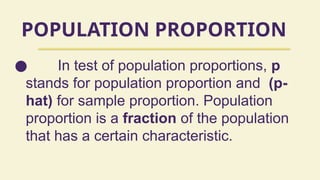
POPULATION PROPORTION
● Intest of population proportions, p
stands for population proportion and (p-
hat) for sample proportion. Population
proportion is a fraction of the population
that has a certain characteristic.
210.
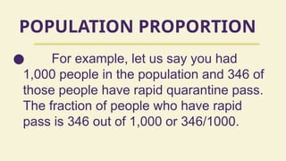
POPULATION PROPORTION
● Forexample, let us say you had
1,000 people in the population and 346 of
those people have rapid quarantine pass.
The fraction of people who have rapid
pass is 346 out of 1,000 or 346/1000.
211.
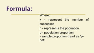
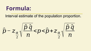
Formula:
Where:
x - representthe number of
successes
n - represents the popuation.
p - population proportion
- sample proportion (read as “p-
hat”
212.
Formula:
^
𝑝− 𝑧𝛼
2 √^
𝑝^
𝑞
𝑛
<𝑝<^
𝑝+𝑧𝛼
2 √^
𝑝 ^
𝑞
𝑛
Interval estimate of the population proportion.
213.
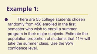
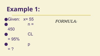
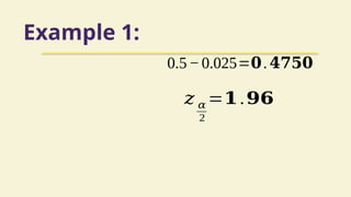
Example 1:
● Thereare 55 college students chosen
randomly from 450 enrolled in the first
semester who wish to enroll a summer
program in their major subjects. Estimate the
population proportion of students that 11% will
take the summer class. Use the 95%
confidence level.
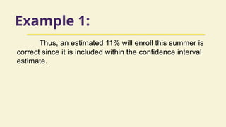
Example 1:
Thus, anestimated 11% will enroll this summer is
correct since it is included within the confidence interval
estimate.
220.
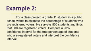
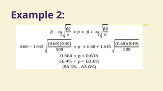
Example 2:
For aclass project, a grade 11 student in a public
school wants to estimate the percentage of students who
are registered voters. He surveys 500 students and finds
that 300 are registered voters. Compute a 90%
confidence interval for the true percentage of students
who are registered voters and interpret the confidence
interval.