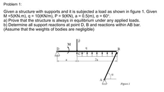
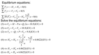
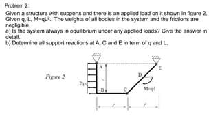
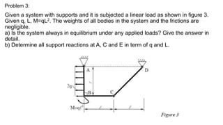
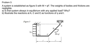
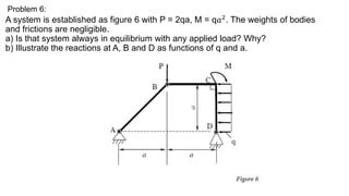
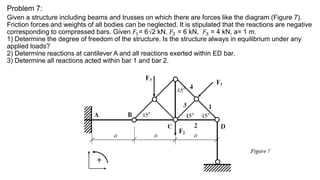
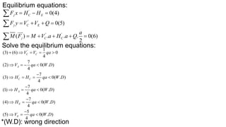
This document contains the homework submission of student Tran Quoc Thai for the Engineering Mechanics course. It includes 6 problems solving statics analysis of different structures. The student provides the free body diagrams, equilibrium equations, and solutions for the support reactions and internal forces of each structure when subjected to various loads.

1. FALCUTY OF APPLIED SCIENCE
ENGINEERING MECHANICS (AS1003)
HOMEWORK SUBMISSION
Group: CC01
Part: 1. Statics
Student’s fullname: Tran Quoc Thai
Stundent’s ID: 2153795
Semester: HK213
Lecturer: Assoc. Prof. Dr. Tich Thien TRUONG
Submission date: Sunday, July 17th, 2022

2. Problem 1:
Given a structure with supports and it is subjected a load as shown in figure 1. Given
M =5(KN.m), q = 10(KN/m), P = 9(KN), a = 0.5(m), α = 60°.
a) Prove that the structure is always in equilibrium under any applied loads.
b) Determine all support reactions at point D, B and reactions within AB bar.
(Assume that the weights of bodies are negligible)

3. Solution:
a)To consider the equilibrium state of the structure, we
compute dof of the system.
This structure is always in equilibrium state under any
applied loads because
b)
1. Consider the equilibrium state for the bar DCB
Release two supports at two positions D and B.
Equilibrium equations:
2. Consider the equilibrium state for the bar AB
Release two supports at two positions A and B
3
1
3. 3.2 (2 2 2) 0
s
j
j
dof n R

      

1 2 .
Q a q

1
1
0(1)
0(2)
( ) . .2 0(3)
j D B
j D B
J B
F x H H
F y V Q P V
M F M P a Q a V
  
    
    



0
dof 

4. '
'
' '
0(4)
0(5)
2 2 3
( ) . . 0(6)
3 3
j A B
j A B
J B B
F x H H
F y V V
M F V a H a
   
   
  



1
'
1
'
'
'
(3) . .2 10.5( ) 0
(5) 10.5( ) 0
(2) 9.5( ) 0
2
.
7 3
3
(6) 6.0622( ) 0
2
2 3
3
(4) 6.0622( ) 0
(1) 6.0622( ) 0
B
B B A
D B
B
B B
A B
D B
V M P a Q a KN
V V V KN
V Q P V KN
V a
H H KN
a
H H KN
H H KN
     
    
      
     
   
   
Equilibrium equations:
Solve the equilibrium equations:

5. Problem 2:
Given a structure with supports and there is an applied load on it shown in figure 2.
Given q, L, M=qL2. The weights of all bodies in the system and the frictions are
negligible.
a) Is the system always in equilibrium under any applied loads? Give the answer in
detail.
b) Determine all support reactions at A, C and E in term of q and L.

6. Solution:
a) To consider the equilibrium state of the structure, we
compute dof of the system.
This structure is always in equilibrium state under any
applied loads because
b)
1. Consider the equilibrium state for the frame ABC
Release two supports at two positions A and C
Equilibrium equations:
2. Consider the equilibrium state for the bar CDE
Release two supports at two positions C and E
3
1
3. 3.2 (2 2 2) 0
s
j
j
dof n R

      

1
1
0(1)
0(2)
( ) . . . 0(3)
2
j A C
j A C
j C C
F x H H Q
F y V V
l
M F Q H l V l
   
   
   



0
dof 

7. '
'
0(4)
0(5)
( ) . . 0(6)
j C E
J C E
j E E
F x H H
F y V V
M F M V l H l
  
   
   



*
'
'
1
(3) (6) 0
(5) 0( . )
(4) 0
(2) 0
(1) 2 0
C
E
C C E
C C A
A
V ql
V ql W D
H H H
V V V ql
H Q ql
   
   
   
    
   
Equilibrium equations:
Solve the equilibrium equations:
*(W.D): wrong direction

8. Problem 3:
Given a system with supports and it is subjected a linear load as shown in figure 3.
Given q, L, M=qL2. The weights of all bodies in the system and the frictions are
negligible.
a) Is the system always in equilibrium under any applied loads? Give the answer in
detail.
b) Determine all support reactions at A, C and E in term of q and L.

9. Solution:
a) To consider the equilibrium state of the structure, we
compute dof of the system.
This structure is always in equilibrium state under any
applied loads because
b)
1. Consider the equilibrium state for the frame ABC
Release two supports at two positions A and C
Equilibrium equations:
2. Consider the equilibrium state for the bar CD
Release two supports at two positions C and D
3
1
3. 3.2 (2 2 2) 0
s
j
j
dof n R

      

0
dof 
1
1
0(1)
0(2)
( ) . . . 0(3)
2
j A C
j A C
j C C
F x H H Q
F y V V
l
M F M Q H l V l
   
   
    




10. '
'
' '
0(4)
0(5)
( ) . . 0(6)
j C D
J C D
j C C
F x H H
F y V V
M F V l H l
  
   
  



'
'
(3) (6) 0
(5) 0( . )
(6) 0( . )
(4) 0( . )
(2) 0
(1) 0
C C
D
C C
D
A
A
V V ql
V ql W D
H H ql W D
H qL W D
V ql
H qL
    
   
    
   
  
  
Equilibrium equations:
Solve the equilibrium equations:
*(W.D): wrong direction

11. Problem 4:
A system is established as figure 4 with AB = 2a = CD = 2CB, F = qa. The weights of
bodies and frictions are negligible.
a) Is that system always in equilibrium with any applied load? Why?
b) Determine the reactions at A and B according to each of the two following
values of M.
- M = (√2q𝑎2 ) / 2
- M = 2qa

12. Solution:
a) To consider the equilibrium state of the structure, we
compute dof of the system.
This structure is not always in equilibrium state under
any applied loads because
b)
1. Consider the equilibrium state for the bar DBC
Release two supports at two positions B and C
• We have:
Equilibrium condition:
The bar DBC must contact the frame AB at position B or
NB > 0
That means:
3
1
3. 3.2 (2 2 0.5) 0.5
s
j
j
dof n R

      
 2
( ) . . .sin 0(1)
2
(2)
j B
B
M F M N BC F DC
qa M
N
a

    

 

2
2
2
2
(2) 0
2 0
2 (3)
qa M
a
qa M
M qa

 
  
 
0
dof 

13. Case 1:  Condition (2) is satisfied, that
means the system is always in equilibrium state under any
applied loads.
Substitute in equation (2) we get
• Consider the equilibrium state for the bar AB
• Release two supports at two positions A and B
Equilibrium equations:
Solve the equilibrium equations:
Case 2:  Condition (2) is not satisfied, that
means the system is not in equilibrium state.So
Then:
2
2
2
qa
M 
2
2
2
qa
M 
2
0
2
B
qa
N  
'
'
1
'
1
sin 0(4)
0(5)
( ) . 2 . cos 0(6)
j A B
j A B
j A B
F x H N
F y V N cos Q
M F M Q a a N



  
   
   



2
1
(4) 0
2
5
(5) 0
2
(6) 3 0
A
A
A
H qa
V qa
M qa
  
  
  
2
2
M qa

2
(4) 0
(5) 2 0
(6) 2
A
A
A
H
V qa
M qa
 
  
 
0
B
N 

14. Problem 5:
A system is established as figure 5 with M = ql2. The weights of bodies and frictions are
negligible.
a) Is that system always in equilibrium with any applied load? Why?
b) Illustrate the reactions at A, C and E as functions of q and l.

15. Solution:
a)To consider the equilibrium state of the structure, we
compute dof of the system.
This structure is always in equilibrium state under any
applied loads because
b)
1. Consider the equilibrium state for the frame ABC
Release two supports at two positions A and C.
Equilibrium equations:
2. Consider the equilibrium state for the bar CD
Release two supports at two positions C and D
3
1
3. 3.2 (2 2 2) 0
s
j
j
dof n R

      

1
1
0(1)
0(2)
( ) . . . 0(3)
2
j A C
j A C
j C C
F x H Q H
F y V V
l
M F Q H l V l
   
   
   



0
dof 
ql

16. '
'
' '
0(4)
0(5)
( ) . . 0(6)
j C E
j C E
j C C
F x H H
F y V V
M F M V l H l
  
   
   



'
'
(3) (6) 0
(5) 0( . )
(6) 0( . )
(4) 0( . )
(2) 0
(1) 0
C C
E
C C
E
A
A
V V ql
V ql W D
H H ql W D
H qL W D
V ql
H qL
    
   
    
   
  
  
Equilibrium equations:
Solve the equilibrium equations:
*(W.D): wrong direction

17. Problem 6:
A system is established as figure 6 with P = 2qa, M = q𝑎2
. The weights of bodies
and frictions are negligible.
a) Is that system always in equilibrium with any applied load? Why?
b) Illustrate the reactions at A, B and D as functions of q and a.

18. Solution:
a)To consider the equilibrium state of the structure, we
compute dof of the system.
This structure is always in equilibrium state under any
applied loads because
b)
1. Consider the equilibrium state for the bar AB
Release two supports at two positions A and B.
Equilibrium equations:
2. Consider the equilibrium state for the frame BCD
Release two supports at two positions B and D
3
1
3. 3.2 (2 2 2) 0
s
j
j
dof n R

      

1 2 .
Q a q

0(1)
0(2)
( ) . . . 0(3)
j A B
j A B
J B B
F x H H
F y V P V
M F H a V a P a
  
   
    



0
dof 
a
a
y
x
a
a
𝑎
2

19. '
'
' '
0(4)
0(5)
( ) . . . 0(6)
2
j B D
j B D
j B C
F x H H Q
F y V V
a
M F M V a H a Q
   
   
    



'
'
7
(3) (6) 0
4
7
(5) 0( . )
4
15
(3) 0
4
15
(2) 0
4
15
(1) 0
4
11
(4) 0
4
B B
D
B B
A
A
D
V V qa
V qa W D
H H qa
V qa
H qa
H qa
    
   
   
  
  
  
Equilibrium equations:
Solve the equilibrium equations:
*(W.D): wrong direction

20. Problem 7:
Given a structure including beams and trusses on which there are forces like the diagram (Figure 7).
Friction forces and weights of all bodies can be neglected. It is stipulated that the reactions are negative
corresponding to compressed bars. Given 𝐹1= 6√2 kN, 𝐹2 = 6 kN, 𝐹3 = 4 kN, a= 1 m.
1) Determine the degree of freedom of the structure. Is the structure always in equilibrium under any
applied loads?
2) Determine reactions at cantilever A and all reactions exerted within ED bar.
3) Determine all reactions acted within bar 1 and bar 2.

21. Problem 8:
Given a structure with their supports on which there are external forces
like figure 8. Neglect friction forces at point D. Given a= 0.6 m, b= 0.4 m,
AD=2BD= 2a, CD=CE=b, P= 600N, Q=2P, q=1000 N/m. Determine all
reactions at cantilever A in two cases:
1) M= 300 Nm
2) M= 600 Nm

22. Solution:
a) To consider the equilibrium state of the structure, we
compute dof of the system.
This structure is not always in equilibrium state under
any applied loads because
b)
1. Consider the equilibrium state for the bar ECD
Release two supports at two positions E and D
Equilibrium equations:
Equilibrium condition:
The bar DBC must contact the frame AB at position B or
ND > 0
That means:
3
1
3. 3.2 (2 3 0.5) 0.5
s
j
j
dof n R

      

0
dof 
1
1
.cos30 0(1)
sin30 0(2)
3
( ) . . .sin30.2 0(3)
2
j E D
j D
j D
F x H N
F y P Q N
M F M P b Q b N b
  
    
    



E
D
y
x
C
P
1
1
1
3
.
2
(3) 0
2.sin30
3
. 0
2
3
. 1200( . )(4)
2
P Q M
P Q M
M P Q N m
 
 
   
   

23. Case 1:  Condition (4) is satisfied, that
means the system is always in equilibrium state under any
applied loads.
Substitute in equation (3) we get
• Consider the equilibrium state for the bar ADB
• Release two supports at two positions A and B
Equilibrium equations:
Solve the equilibrium equations:
Case 2:  Condition (4) is satisfied, that
means the system is always in equilibrium state under any
applied loads.
Substitute in equation (3) we get
300( . )
M N m

300
M  900( )
D
N N

'
'
' '
sin30 .cos30 0(5)
cos30 .sin30 0(6)
( ) .3 sin30. 3 cos30. 0(7)
j A D
j A D
j A D D
F x H N Q
F y V N Q
M F M Q a N a N a
   
   
    



(5) 1489.23 0 .
(6) 1379.42 0
(7) 2160 0
A
A
A
H W D
V
M
    
  
  
600( . )
M N m

(5) 1339.23 0 .
(6) 1119.62 0
(7) 2160 0
A
A
A
H W D
V
M
    
  
  
600
M  600( )
D
N N


24. Problem 9:
Given a mechanical structure includes their supports on which there are
external forces like figure 9. Given q, a, P= 2qa and M= q𝑎2 and all friction
forces and weights of bodies are negligible. Determine all reactions at A.
C and E in terms of q and a.

25. Solution:
a) To consider the equilibrium state of the structure, we
compute dof of the system.
This structure is always in equilibrium state under any
applied loads because
b)
1. Consider the equilibrium state for the frame ABC
Release two supports at two positions A and C
Equilibrium equations:
2. Consider the equilibrium state for the frame CDE
Release two supports at two positions C and E
3
1
3. 3.2 (2 2 2) 0
s
j
j
dof n R

      

0
dof 
0(1)
0(2)
( ) . . . 0(3)
j A C
j A C
j C C
F x H H
F y V P V
M F H a P a V a
  
   
    



A
B
C
y
x
a
a
C
E
D
M
y
x
a
a

26. '
'
' '
0(4)
0(5)
( ) . . . 0(6)
2
j C E
j C E
j C C
F x H H
F y V V Q
a
M F M V a H a Q
  
   
    



'
'
1
(3) (6) 0
4
7
(2) 0( . )
4
7
(3) 0( . )
4
7
(1) 0( . )
4
7
(4) 0( . )
4
5
(5) 0( . )
4
C C
A
C C
A
E
E
V V qa
V qa W D
H H qa W D
H qa W D
H qa W D
V qa W D
    
   

   

  

  

  
Equilibrium equations:
Solve the equilibrium equations:
*(W.D): wrong direction

27. Problem 10:
A mechanical system is shown as in figure 10 with a = 0.6 m, b = 0.4 m, AB = 2a, P =
600 N, CB = BD = DE = b, q = 1000 N/m. Friction at B is negligible. Determine the
reactions at support A corresponding to each of the following conditions.
1) M = 500 Nm
2) M = 700 Nm

28. Solution:
a) To consider the equilibrium state of the structure, we
compute dof of the system.
This structure is not always in equilibrium state under
any applied loads because
b)
1. Consider the equilibrium state for the bar EDBC
Release two supports at two positions E and B
• We have:
Equilibrium condition: The bar EDBC must contact the bar
AB at position B or NB > 0
That means:
3
1
3. 3.2 (2 2 0.5) 0.5
s
j
j
dof n R

      

5
( ) . .2 . 0(1)
2
5
. .
2 (2)
2
j B
B
M F M P b N b Q b
P b Q b M
N
b
    
 
 

5
. .
2
(2) 0
2
5
. . 0
2
160(3)
P b Q b M
b
P b Q b M
M
 
 
   
  
0
dof 
E D B C
x
y
P
M
b b
b
Q
5b/2
𝑁𝐵
𝑉𝐸
𝐻𝐵

29. Case 1:  Condition (3) not is satisfied, that
means the system is not in equilibrium state under any
applied loads.
That means
• Consider the equilibrium state for the bar AB
• Release two supports at two positions A and B
Equilibrium equations:
Solve the equilibrium equations:
Case 2:  Condition (3) is not satisfied, that
means the system is not in equilibrium state under any
applied loads.
That means
500( . )
M N m

0( )
B
N N

0(4)
0(5)
( ) 0(6)
j A
j A
j A
F x H
F y V
M F M
 
 
 



(4) 0
(5) 0
(6) 0
A
A
A
H
V
M
 
 
 
600( . )
M N m

(5) 0
(6) 0
(7) 0
A
A
A
H
V
M
 
 
 
0( )
D
N N

y
x
A
B
𝑁𝐵
′

30. Problem 11:
A mechanical system is shown as in figure 11 with R = 2r = 1 m; 𝛼 = 60°,
AB = 3m, P = 2 KN, Q = 1 KN, M = 1.5 KNm.
Determine the reactions at A and the tensile force at E. The friction at
external pin B is negligible