The document contains the results of validity and reliability tests for variables measuring work environment (X), job satisfaction (Y), and turnover intention (Z). It reports correlations between variables and the items measuring each variable. It also reports Cronbach's alpha coefficients for each set of items. Further, it contains the results of regression and correlation analyses examining the relationships between the variables. It tests the assumptions of multicollinearity, heteroscedasticity, and linearity for the regression models.

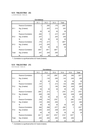
1. UJI VALIDITAS (X)
LINGKUNGAN KERJA
Correlations
X1.1 X1.2 X1.3 Total
X1.1
Pearson Correlation 1 ,092 ,175 ,493**
Sig. (2-tailed) ,437 ,312 ,001
N 35 35 35 35
X1.2
Pearson Correlation ,092 1 ,217 ,491**
Sig. (2-tailed) ,437 ,203 ,004
N 35 35 35 35
X1.3
Pearson Correlation ,175 ,217 1 ,687**
Sig. (2-tailed) ,312 ,203 ,000
N 35 35 35 35
Total
Pearson Correlation ,493**
,491**
,687**
1
Sig. (2-tailed) ,001 ,004 ,000
N 35 35 35 35
**. Correlation is significantatthe 0.01 level (2-tailed).
UJI VALIDITAS (Y)
KEPUASAN KERJA
Correlations
Y1.1 Y1.2 Y1.3 Y1.4 Y1.5 Total
Y1.1
Pearson Correlation 1 ,137 ,358**
,238 ,362 ,521**
Sig. (2-tailed) ,132 ,000 ,143 ,042 ,000
N 35 35 35 35 35 35
Y1.2
Pearson Correlation ,137 1 ,213 ,142 ,098 ,443**
Sig. (2-tailed) ,132 ,185 ,094 ,424 ,002
N 35 35 35 35 35 35
Y1.3
Pearson Correlation ,358**
,213 1 ,379**
,377*
,672**
Sig. (2-tailed) ,000 ,185 ,004 ,038 ,000
N 35 35 35 35 35 35
Y1.4
Pearson Correlation ,238 ,142 ,379**
1 ,296*
,514**
Sig. (2-tailed) ,143 ,094 ,004 ,031 ,000
N 35 35 35 35 35 35
Y1.5
Pearson Correlation ,362 ,098 ,377*
,296*
1 ,537**
Sig. (2-tailed) ,042 ,424 ,038 ,031 ,000
N 35 35 35 35 35 35
Total
Pearson Correlation ,521**
,443**
,672**
,514**
,537**
1
Sig. (2-tailed) ,000 ,002 ,000 ,000 ,000
N 35 35 35 35 35 35
**. Correlation is significantatthe 0.01 level (2-tailed).

2. UJI VALIDITAS (Z)
TURNOVER INTANTION
Correlations
Y1.1 Y1.2 Y1.3 Y1.4 Total
Y1.1
Pearson Correlation 1 ,118 ,375**
,265 ,571**
Sig. (2-tailed) ,076 ,000 ,053 ,000
N 35 35 35 35 35
Y1.2
Pearson Correlation ,118 1 ,105 ,294 ,537**
Sig. (2-tailed) ,076 ,295 ,041 ,000
N 35 35 35 35 35
Y1.3
Pearson Correlation ,375**
,105 1 ,369**
,673**
Sig. (2-tailed) ,000 ,295 ,005 ,000
N 35 35 35 35 35
Y1.4
Pearson Correlation ,265 ,294 ,369**
1 ,524**
Sig. (2-tailed) ,053 ,041 ,005 ,000
N 35 35 35 35 35
Total
Pearson Correlation ,571**
,537**
,673**
,524**
1
Sig. (2-tailed) ,000 ,000 ,000 ,000
N 35 35 35 35 35
**. Correlation is significantatthe 0.01 level (2-tailed).

3. UJI RELIABILITAS (X)
LINGKUNGAN KERJA
RELIABILITY
/VARIABLES=X1.1 X1.2 X1.3 TOTAL
/SCALE('ALL VARIABLES') ALL
/MODEL=ALPHA
/STATISTICS=DESCRIPTIVE SCALE HOTELLING CORR
/SUMMARY=TOTAL CORR.
Reliability
Scale: ALL VARIABLES
Case Processing Summary
N %
Cases
Valid 35 100,0
Excludeda
0 ,0
Total 35 100,0
a. Listwise deletion based on all variables in the
procedure.
Reliability Statistics
Cronbach's
Alpha
N of Items
,684 3
UJI RELIABILITAS (Y)
KEPUASAN KERJA
RELIABILITY
/VARIABLES=Y1..1 Y1.2 Y1.3 Y1.4 Y1.5 TOTAL
/SCALE('ALL VARIABLES') ALL
/MODEL=ALPHA
/STATISTICS=DESCRIPTIVE SCALE HOTELLING CORR
/SUMMARY=TOTAL CORR.
Reliability
Scale: ALL VARIABLES
Case Processing Summary
N %
Cases
Valid 35 100,0
Excludeda
0 ,0
Total 35 100,0

4. a. Listwise deletion based on all variables in the
procedure.
Reliability Statistics
Cronbach's
Alpha
N of Items
,691 5
UJI RELIABEL (Z)
TURNOVER INTANTION
RELIABILITY
/VARIABLES=Z1.1 Z1.2 Z1.3 Z1.4 TOTAL
/SCALE('ALL VARIABLES') ALL
/MODEL=ALPHA
/STATISTICS=DESCRIPTIVE SCALE HOTELLING CORR
/SUMMARY=TOTAL CORR.
Reliability
Scale: ALL VARIABLES
Case Processing Summary
N %
Cases
Valid 35 100,0
Excludeda
0 ,0
Total 35 100,0
a. Listwise deletion based on all variables in the
procedure.
Reliability Statistics
Cronbach's
Alpha
N of Items
,655 4

5. UJI NORMALITAS DATA
One-Sample Kolmogorov-Smirnov Test
Lingkungan
Kerja
Kepuasan
Kerja
Turnover
Intentions
N 35 35 35
Normal Parametersa
Mean 21.5581 24.6047 9.3023
Std. Deviation 1.77687 2.76147 1.80653
Most Extreme Differences Absolute .156 .191 .139
Positive .146 .191 .127
Negative -.156 -.170 -.139
Kolmogorov-SmirnovZ 1.025 1.255 .909
Asymp. Sig. (2-teiled) .244 .086 .380
a.Test distribution is Normal.
ANALISIS DATA (PATH ANALYSIS)
REGRESI MODEL I
REGRESSION
/MISSING LISTWISE
/STATISTICS COEFF OUTS R ANOVA
/CRITERIA=PIN(.05) POUT(.10)
/NOORIGIN
/DEPENDENT Y
/METHOD=ENTER X.
Regression
[DataSet0]
Variables Entered/Removeda
Model Variables Entered Variables
Removed
Method
1
Lingkungan Kerja
(X)b
. Enter
a. DependentVariable:Kepuasan Kerja (Y)
b. All requested variables entered.
Model Summary
Model R R Square Adjusted R
Square
Std. Error of the
Estimate
1 .459a
.225 .204 2.51389

6. a. Predictors:(Constant),Lingkungan Kerja (X)
ANOVAa
Model Sum of
Squares
df Mean
Square
F Sig.
1
Regression 6.969 1 6.969 9.581 .000a
Residual 70.631 33 2.141
Total 77.600 34
a. DependentVariable:Kepuasan Kerja (Y)
b. Predictors:(Constant),Lingkungan Kerja (X)
Coefficientsa
Model Unstandardized
Coefficients
Standardized
Coefficients
T Sig.
B Std. Error Beta
1
(Constant) 9.888 1.911 5.175 .000
Lingkungan Kerja (X) .439 .196 .329 2.239 .010
a. DependentVariable:Kepuasan Kerja (Y)
REGRESI MODEL II
REGRESSION
/MISSING LISTWISE
/STATISTICS COEFF OUTS R ANOVA
/CRITERIA=PIN(.05) POUT(.10)
/NOORIGIN
/DEPENDENT Z
/METHOD=ENTER X Y.
Regression
[DataSet0]
Variables Entered/Removeda
Model Variables Entered Variables
Removed
Method
1
Kepuasan Kerja
(Y), Lingkungan
Kerja (X)b
. Enter

7. a. DependentVariable:Turnover Intantion (Z)
b. All requested variables entered.
Model Summary
Model R R Square Adjusted R
Square
Std. Error of the
Estimate
1 .847a
.661 .602 3.19186
a. Predictors:(Constant),Kepuasan Kerja (Y), Lingkungan Kerja (X)
ANOVAa
Model Sum of
Squares
Df Mean Square F Sig.
1
Regression 12.943 2 6.472 31.197 .000a
Residual 35.457 32 1.108
Total 48.400 34
a. DependentVariable:Turnover Intantion (Z)
b. Predictors:(Constant),Kepuasan Kerja (Y), Lingkungan Kerja (X)
Coefficientsa
Model Unstandardized
Coefficients
Standardized
Coefficients
t Sig.
B Std. Error Beta
1
(Constant) 9.229 1.775 5.199 .000
Lingkungan Kerja (X) .226 .088 .445 2.568 .007
Kepuasan Kerja (Y) .359 .091 .507 3.945 .000
a. DependentVariable:Turnover Intantion (Z)

8. UJI ASUMSI KLASIK
MULTIKOLINIERITAS
Persamaan Pertama
Coefficientsa
Model Unstandardized
Coefficients
Standardized
Coefficients
t Sig. Collinearity
Statistics
B Std. Error Beta Tolerance VIF
1
(Constant) 9.888 1.911 5.175 .000
Lingkungan Kerja (X) .439 .196 .329 2.239 .010 1.000 1.000
a. DependentVariable:Kepuasan Kerja (Y)
Coefficient Correlationsa
Model Lingkungan
Kerja (X)
1
Correlations Lingkungan Kerja (X) 1.000
Covariances Lingkungan Kerja (X) .046
a. DependentVariable:Kepuasan Kerja (Y)
Collinearity Diagnosticsa
Model Dimension Eigenvalue Condition Index Variance Proportions
(Constant) Lingkungan
Kerja (X)
1
1 1.996 1.000 .00 .00
2 .004 22.707 .92 .10
a. DependentVariable:Kepuasan Kerja (Y)
Persamaan Kedua
Coefficientsa
Model Unstandardized
Coefficients
Standardized
Coefficients
t Sig. Collinearity
Statistics
B Std. Error Beta Tolerance VIF
1
(Constant) 9.229 1.775 5.199 .000
Lingkungan Kerja (X) .226 .088 .445 2.568 .007 .870 1.126
Kepuasan Kerja (Y) .359 .091 .507 3.945 .000 .718 1.278
a. DependentVariable:Turnover Intantion (Z)

9. Coefficient Correlationsa
Model Kepuasan Kerja
(Y)
Lingkungan
Kerja (X)
1
Correlations
Kepuasan Kerja (Y) 1.000 .019
Lingkungan Kerja (X) .019 1.000
Covariances
Kepuasan Kerja (Y) .049 .004
Lingkungan Kerja (X) .004 .049
a. DependentVariable:Turnover Intantion (Z)
Collinearity Diagnosticsa
Model Dimension Eigenvalue Condition Index Variance Proportions
(Constant) Lingkungan
Kerja (X)
Kepuasan Kerja
(Y)
1
1 2.990 1.000 .00 .00 .00
2 .008 19.359 .04 .52 .33
3 .002 39.802 .97 .48 .67
a. DependentVariable:Turnover Intantion (Z)
HETEROSKEDASTISITAS
Persamaan Pertama
Coefficientsa
Model Unstandardized
Coefficients
Standardized
Coefficients
t Sig.
B Std. Error Beta
1
(Constant) 2.548 3.211 .793 .380
Lingkungan Kerja (X) .139 .196 .129 .709 .413
a. DependentVariable:ABS_RESID
Persamaan Kedua
Coefficientsa
Model Unstandardized
Coefficients
Standardized
Coefficients
t Sig.
B Std. Error Beta
1
(Constant) 1.003 1.121 .894 .465
Lingkungan_Kerja .087 .116 .426 .750 .432
Kepuasan_Kerja .086 .132 .204 .652 .358
a. DependentVariable:ABS_RESID

10. UJI LINIERITAS PERSAMAAN I
MEANS TABLES=kpuasn BY link_krj trnver
/CELLS MEAN COUNT STDDEV
/STATISTICS LINEARITY.
[DataSet0]
Case Processing Summary
Cases
Included Excluded Total
N Percent N Percent N Percent
Kepuasan Kerja * Lingkungan Kerja 35 100.0% 0 0.0% 35 100.0%
Kepuasan Kerja * Turnover Intetion 35 100.0% 0 0.0% 35 100.0%
Kepuasan Kerja * Lingkungan Kerja
Report
Kepuasan Kerja
Lingkungan Kerja Mean N Std. Deviation
10 18.00 1 .
11 19.88 8 2.100
12 19.00 11 1.000
13 19.27 11 1.555
14 18.67 3 1.528
15 18.00 1 .
Total 19.20 35 1.511

11. ANOVA Table
Sum of
Squares
Df Mean
Square
F Sig.
Kepuasan Kerja *
Lingkungan Kerja
Between Groups
(Combined) 107.877 5 21.575 6.655 .000
Linearity 81.969 1 81.969 17.819 .000
Deviation from
Linearity
25.908 4 6.477 1.614 .006
Within Groups 89.723 29 3.094
Total 305.477 34
Measures of Association
R R Squared Eta Eta Squared
Kepuasan Kerja * Lingkungan Kerja .559 .325 .619 .402
Kepuasan Kerja * Turnover_Intetion
Report
Kepuasan Kerja
Turnover_Intetion Mean N Std. Deviation
12 17.00 1 .
14 19.80 5 1.483
15 19.33 15 1.759
16 19.14 7 1.215
17 19.00 6 1.265
18 18.00 1 .
Total 19.20 35 1.511
ANOVA Table
Sum of
Squares
Df Mean
Square
F Sig.
Kepuasan Kerja * Between Groups (Combined) 128.610 5 25.722 7.724 .000

12. Turnover_Intetion Linearity 101.162 1 101.162 19.068 .000
Deviation from
Linearity
68.448 3 22.816 1.888 .004
Within Groups 98.990 29 3.414
Total 397.210 34
Measures of Association
R R Squared Eta Eta Squared
Kepuasan Kerja *
Turnover_Intetion
.546 .302 .633 .511
UJI LINIERITAS PERSAMAAN II
MEANS TABLES=trnver BY link_krj kpuasn
/CELLS MEAN COUNT STDDEV
/STATISTICS LINEARITY.
DataSet0]
Case Processing Summary
Cases
Included Excluded Total
N Percent N Percent N Percent
Turnover_Intetion *
Lingkungan Kerja
35 100.0% 0 0.0% 35 100.0%
Turnover_Intetion *
Kepuasan Kerja
35 100.0% 0 0.0% 35 100.0%

13. Turnover_Intetion * Lingkungan Kerja
Report
Turnover_Intetion
Lingkungan Kerja Mean N Std. Deviation
10 15.00 1 .
11 14.88 8 1.642
12 15.55 11 .820
13 15.55 11 1.293
14 15.33 3 .577
15 17.00 1 .
Total 15.40 35 1.193
ANOVA Table
Sum of
Squares
Df Mean
Square
F Sig.
Turnover_Intetion *
Lingkungan Kerja
Between Groups
(Combined) 165.404 5 33.081 8.729 .000
Linearity 142.941 1 142.941 19.984 .000
Deviation from
Linearity
62.463 4 15.616 2.415 .002
Within Groups 92.996 29 3.207
Total 463.804 34
Measures of Association
R R Squared Eta Eta Squared
Turnover_Intetion *
Lingkungan Kerja
.647 .461 .734 .512

14. Turnover_Intetion * Kepuasan Kerja
Report
Turnover_Intetion
Kepuasan Kerja Mean N Std. Deviation
17 14.50 4 1.732
18 16.00 8 1.414
19 15.45 11 .820
20 15.20 5 1.304
21 15.75 4 .957
22 14.50 2 .707
23 15.00 1 .
Total 15.40 35 1.193
ANOVA Table
Sum of
Squares
Df Mean
Square
F Sig.
Turnover_Intetion *
Kepuasan Kerja
Between Groups
(Combined) 188.623 6 31.437 11.012 .438
Linearity 123.101 1 123.101 15.071 .792
Deviation from
Linearity
88.522 5 17.704 2.200 .335
Within Groups 101.777 28 3.634
Total 502.023 34
Measures of Association
R R Squared Eta Eta Squared
Turnover_Intetion * Kepuasan
Kerja
.546 .302 .622 .478