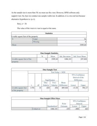
This term paper on SPSS presents statistical analyses related to real estate properties, including frequency distributions, descriptive statistics, correlation analysis, and multiple regression analysis. The study finds significant correlations between various properties metrics, such as a strong correlation between livable square feet and market price. The paper was prepared by Group 8 of the MBA 2021 batch at Bangladesh University of Professionals as part of a business statistics course.

1. Page | i
0
Term paper
On
SPSS
Course Code: BUS 5204
Course Title: Business Statistics
Submitted To:
Tahmina Sultana
Assistant Professor
Dept. of Management, FBS
Bangladesh University of Professionals
Submitted By: (Group-8)
Batch: MBA 2021
Department of Business Administration-General
Submitted Date: 29th
May 2022
Name ID Contribution
Md. Muniruzzaman 2123021043 Data Entry & 8
Jahid Khan Rahat 2123021047 7 & 8
Khan Mehedi Hasan 2123021008 6
MD. Shahajalal Mia 2123021049 5
Tonmoy Paul 2123021045 4
MD. Muzammel Haque 2123021041 3

2. Page | ii
Letter of Transmittal
18th
May 2022
Tahmina Sultana
Assistant Professor
Bangladesh University of Professionals
Subject: Submission of the Term paper on “SPSS”.
Dear Ma’am,
It is a great pleasure and privilege to present the Term paper on “SPSS” which was assigned to us
as a partial requirement for the completion of Business Statistics course. Throughout the study we
tried with the best of our capacity to accommodate as much information and relevant issues as
possible and tried to follow the instructions as you have suggested. We tried our best to make this
term paper as much informative as possible. We sincerely believe that it will satisfy your
requirements. However, we sincerely believe that this report will serve the purpose of our term
paper.
We, therefore, pray and hope that you would kindly accept our term paper and oblige thereby.
With thanks, and best regards.
Sincerely yours,
Members of Group 8
MBA 2021

3. Page | iii
Acknowledgement
We are thankful and pay our deep gratitude towards the almighty Allah at the beginning because
without the blessing we have been this fortunate to finish this term paper. There are a lot of
people whom we wouldn’t to thank too. First of all, our cordial thanks go to Tahmina Sultana
Ma’am as our course instructor to provide us this great opportunity to work in this term paper
and giving us the such privilege to learn thereby. It was a great pleasure for us to work in this
topic. We had a great chance to learn many pros and cons of the topic. In addition, we have learn
about the proper uses of SPSS software.

4. Page | iv
Table of Contents
1. Screenshot of the template variable view ..................................................................................... 1
2. Screenshot of the template data view ........................................................................................... 2
3. Construct a frequency distribution .........................................................................................3
4. Represent the descriptive statistics................................................................................................ 5
5. 4 pairs of variables, run correlation analysis and interpretation.................................................. 6
6. Multiple regression analysis ........................................................................................................ 11
7. One Sample Mean Test (P-value and confidence interval).......................................................... 13
8. Perform Chi-square test for independent variable...................................................................... 20
Appendix Table................................................................................................................. 24

5. Page | 1
1. Screenshot of the template variable view:

6. Page | 2
2. Screenshot of the template data view:

7. Page | 3
3. Construct a frequency distribution:
Frequency Distribution for the mentioned variable (Agent, Bedrooms, Garage, Mortgage Type,
Default) is constructed below:
Statistics
Name of the
real estate
agent
Number of
bedrooms
Does the
home have an
attached
garage?(1=ye
s,0=no)
Fixed or
adjustable.
(Fixed
mortgage 30
years @3%/
first 5 years
+@1%/from 6
year
Is the
mortgage loan
in
default?(1=ye
s,0=no)
N Valid 36 36 36 36 36
Missing 0 0 0 0 0
Mean 3.86 .78 .25 .50
Median 3.00 1.00 .00 .50
Mode 3 1 0 0a
Std. Deviation 1.693 .422 .439 .507
Variance 2.866 .178 .193 .257
Skewness .679 -1.395 1.206 .000
Std. Error of
Skewness
.393 .393 .393 .393
Kurtosis -.575 -.060 -.582 -2.121
Std. Error of
Kurtosis
.768 .768 .768 .768
Minimum 2 0 0 0
Maximum 8 1 1 1
a. Multiple modes exist. The smallest value is shown
Frequency Table
Name of the real estate agent
Frequency Percent Valid Percent Cumulative Percent
Valid Peterson 11 30.6 30.6 30.6
Rose 3 8.3 8.3 38.9
Marty 6 16.7 16.7 55.6
Carter 11 30.6 30.6 86.1
Isaacs 5 13.9 13.9 100.0
Total 36 100.0 100.0

8. Page | 4
Number of bedrooms
Frequency Percent Valid Percent Cumulative Percent
Valid 2 9 25.0 25.0 25.0
3 10 27.8 27.8 52.8
4 6 16.7 16.7 69.4
5 2 5.6 5.6 75.0
6 7 19.4 19.4 94.4
7 1 2.8 2.8 97.2
8 1 2.8 2.8 100.0
Total 36 100.0 100.0
Does the home have an attached garage?(1=yes,0=no)
Frequency Percent Valid Percent Cumulative Percent
Valid No 8 22.2 22.2 22.2
Yes 28 77.8 77.8 100.0
Total 36 100.0 100.0
Fixed or adjustable. (Fixed mortgage 30 years @3%/ first 5 years +@1%/from 6 year
Frequency Percent Valid Percent Cumulative Percent
Valid Adjustable 27 75.0 75.0 75.0
Fixed 9 25.0 25.0 100.0
Total 36 100.0 100.0
Is the mortgage loan in default?(1=yes,0=no)
Frequency Percent Valid Percent Cumulative Percent
Valid No 18 50.0 50.0 50.0
Yes 18 50.0 50.0 100.0
Total 36 100.0 100.0

9. Page | 5
4. Represent the descriptive statistics:
The descriptive statistics (Mean, Median, Mode, Minimum, Maximum, Variance, Standard
Deviation, Skewness, Kurtosis) for Price, Size, Baths, Days, Years, FICO are represented
Below:
Descriptive Statistics
N
Minim
um
Maxi
mum Mean
Std.
Deviatio
n Skewness Kurtosis
Statisti
c
Statisti
c
Statisti
c
Statisti
c Statistic
Statisti
c
Std.
Error
Statisti
c
Std.
Error
Market price in
dollars
36 19029
1
91948
0
369314
.94
176483.0
80
1.769 .393 3.117 .768
Livable square
feet of the
property
36 1650 7670 3509.4
4
1486.101 1.224 .393 1.233 .768
Number of
bathrooms
36 1.5 5.5 2.750 1.1433 .676 .393 -.529 .768
Number of days of
the property on the
market
36 11 58 31.94 10.409 .298 .393 .662 .768
The number of
years that the
mortgage loan has
been paid
36 1 19 6.64 4.661 1.363 .393 1.643 .768
The credit score of
the mortgage loan
holder. HS: 850;
AS: 680, LS:
below 680.
36 583 824 664.83 95.418 .980 .393 -1.008 .768
Valid N (listwise) 36

10. Page | 6
5. 4 pairs of variables, run correlation analysis and interpretation:
I. Correlations analysis and interpretation Size and Price
Descriptive Statistics
Mean Std. Deviation N
Livable square feet of the property 3509.44 1486.101 36
Market price in dollers 369314.94 176483.080 36
Correlations
Livable square
feet of the
property
Market price in
dollers
Livable square feet of the
property
Pearson Correlation 1 .956**
Sig. (2-tailed) <.001
Sum of Squares and Cross-
products
77297388.889 8775227558.889
Covariance 2208496.825 250720787.397
N 36 36
Market price in dollers Pearson Correlation .956**
1
Sig. (2-tailed) <.001
Sum of Squares and Cross-
products
8775227558.889 1090119709027.
889
Covariance 250720787.397 31146277400.79
7
N 36 36
**. Correlation is significant at the 0.01 level (2-tailed).
Interpretation: There is a strong positive correlation between the livable square feet of property
and, the market price in dollars, the p-value is statistically significant.
We have found that r = .956
The degree of relationship is strong as the value of the coefficient is close to +1
So there exists a strong positive correlation between the variables.

11. Page | 7
II. Correlations analysis and interpretation Price and Pool
Descriptive Statistics
Mean Std. Deviation N
Market price in dollers 369314.94 176483.080 36
Does the home have a pool?(1=yes,
0=no)
.61 .494 36
Correlations
Market price in
dollers
Does the home
have a
pool?(1=yes,
0=no)
Market price in dollers Pearson Correlation 1 .101
Sig. (2-tailed) .560
Sum of Squares and Cross-
products
1090119709027.
889
307019.222
Covariance 31146277400.79
7
8771.978
N 36 36
Does the home have a
pool?(1=yes, 0=no)
Pearson Correlation .101 1
Sig. (2-tailed) .560
Sum of Squares and Cross-
products
307019.222 8.556
Covariance 8771.978 .244
N 36 36
Interpretation: There is a weak positive correlation between the price in dollars and the pool of
property, and the p-value is statistically significant.
We have found that r = .101
The degree of relationship is weak as the value of the coefficient is not close to +1 and it is close
to zero.
So there exists a weak positive correlation between the variables.

12. Page | 8
III. Correlations analysis and interpretation Pool and Garage
Descriptive Statistics
Mean Std. Deviation N
Does the home have a pool?(1=yes,
0=no)
.61 .494 36
Does the home have an attached
garage?(1=yes,0=no)
.78 .422 36
Correlations
Does the home
have a
pool?(1=yes,
0=no)
Does the home
have an attached
garage?(1=yes,0
=no)
Does the home have a
pool?(1=yes, 0=no)
Pearson Correlation 1 -.015
Sig. (2-tailed) .930
Sum of Squares and Cross-
products
8.556 -.111
Covariance .244 -.003
N 36 36
Does the home have an
attached garage?(1=yes,0=no)
Pearson Correlation -.015 1
Sig. (2-tailed) .930
Sum of Squares and Cross-
products
-.111 6.222
Covariance -.003 .178
N 36 36
Interpretation: There is a strongly weak negative correlation between the pool and the
garage of property, and the p-value is statistically significant.
We have found that r = -.015
The degree of relationship is strongly weak as the value of the coefficient is close to -1.
So there exists a strongly weak positive correlation between the variables.

13. Page | 9
IV. Correlations analysis and interpretation Bedroom and bathroom
Correlations
Number of
bedrooms
Number of
bathrooms
Number of bedrooms Pearson Correlation 1 .985**
Sig. (2-tailed) <.001
Sum of Squares and Cross-
products
100.306 66.750
Covariance 2.866 1.907
N 36 36
Number of bathrooms Pearson Correlation .985**
1
Sig. (2-tailed) <.001
Sum of Squares and Cross-
products
66.750 45.750
Covariance 1.907 1.307
N 36 36
**. Correlation is significant at the 0.01 level (2-tailed).
Interpretation: There is a strong positive correlation between the Bedroom and the bathroom,
the p-value is statistically significant.
We have found that r = .985
The degree of relationship is strong as the value of the coefficient is close to +1
So there exists a strong positive correlation between the variables.
Descriptive Statistics
Mean Std. Deviation N
Number of bedrooms 3.86 1.693 36
Number of bathrooms 2.750 1.1433 36

14. Page | 10
V. Correlations analysis and interpretation Mortgage and default
Descriptive Statistics
Mean Std. Deviation N
Fixed or adjustable. (Fixed mortgage 30
years @3%/ first 5 years +@1%/from 6
year
.25 .439 36
Is the mortgage loan in
default?(1=yes,0=no)
.50 .507 36
Correlations
Fixed or
adjustable.
(Fixed mortgage
30 years @3%/
first 5 years
+@1%/from 6
year
Is the mortgage
loan in default?
(1=yes,0=no)
Fixed or adjustable. (Fixed
mortgage 30 years @3%/
first 5 years +@1%/from 6
year
Pearson Correlation 1 -.577**
Sig. (2-tailed) <.001
Sum of Squares and Cross-
products
6.750 -4.500
Covariance .193 -.129
N 36 36
Is the mortgage loan in
default?(1=yes,0=no)
Pearson Correlation -.577**
1
Sig. (2-tailed) <.001
Sum of Squares and Cross-
products
-4.500 9.000
Covariance -.129 .257
N 36 36
**. Correlation is significant at the 0.01 level (2-tailed).
Interpretation: There is a moderately weak negative correlation between the Mortgage and the
default, and the p-value is statistically significant.
We have found that r = -.577
The degree of relationship is moderately weak as the value of the coefficient is not close to -1 and
is not close to zero.
So there exists a strongly weak positive correlation between the variables.

15. Page | 11
6. Multiple regression analysis:
The dependent variable is Price and the independent variables are Size, Bedrooms, Days,
Township, Years, and FICO
Model Summary
Model R R Square Adjusted R Square
Std. Error of the
Estimate
1 .963a
.927 .912 52315.347
a. Predictors: (Constant), The credit score of the mortgage loan holder. HS: 850; AS: 680, LS:
below 680., Area where the property is located, Livable square feet of the property, Number of
days of the property on the market, The number of years that the mortgage loan has been paid,
Number of bedrooms
As indicated in match summary, we can see that R-square value is .927, which means that our
independent variables cause 92,7% change in the dependent variables.
ANOVAa
Model Sum of Squares df Mean Square F Sig.
1 Regression 1010749738464.
263
6 168458289744.0
44
61.551 <.001b
Residual 79369970563.62
5
29 2736895536.677
Total 1090119709027.
889
35
a. Dependent Variable: Market price in dollers
b. Predictors: (Constant), The credit score of the mortgage loan holder. HS: 850; AS: 680, LS:
below 680., Area where the property is located, Livable square feet of the property, Number of
days of the property on the market, The number of years that the mortgage loan has been paid,
Number of bedrooms
Anova result shows that P-value is <0.000, which is less than 0.05 hence, we say that there is a
significant relationship between our independent variables and dependent variable.

16. Page | 12
Coefficients
Model
Unstandardized
Coefficients
Standardized
Coefficients
t Sig.
B Std. Error Beta
1 (Constant) -56729.335 79604.363 -.713 .482
Livable square feet of
the property
110.539 15.115 .931 7.313 <.001
Number of bedrooms 2511.881 13562.002 .024 .185 .854
Number of days of the
property on the market
1774.393 999.234 .105 1.776 .086
Area where the property
is located
3361.690 7168.430 .024 .469 .643
The number of years that
the mortgage loan has
been paid
129.309 2467.373 .003 .052 .959
The credit score of the
mortgage loan holder.
HS: 850; AS: 680, LS:
below 680.
-59.821 118.326 -.032 -.506 .617
a. Dependent Variable: Market price in dollars
As indicate that beta value is .931, .024, .105, .024, .003, -.032, which means that change of
independent variables by one unit will bring about change in the dependent variable by .931, .024,
.105, .024, .003, -.032, unit.
Furthermore, the beta is positive, which indicate the positive relationship between market price in
dollars and size, bedrooms, days township, years and FICO or you can say that when market price
of dollar increase also size, bedrooms, days township, years will also increase by.931, .024, .105,
. Let,
Market price in dollars = Y
Livable square feet of the property = 𝑋1
Number of bedrooms = 𝑋2
Number of the day of the property on the market = 𝑋3
Area where the property is located = 𝑋4

17. Page | 13
The number of years that the mortgage loan has been paid = 𝑋5
The credit score of the mortgage loan holder = 𝑋6
So, the regression model is
Y=-56729.335+110.539×𝑿𝟏+2511.881×𝑿𝟐+3361.690×𝑿𝟑+3361.690×𝑿𝟒+129.309×𝑿𝟓+(-59.821)×𝑿6
7. One Sample Mean Test (P-value and confidence interval)
I. For size variable
We calculate one sample mean test for “Size” for this we assume a population means is 3020
Here,
Null Hypothesis: The sample mean is not significantly different from the hypothesized
population mean.
Alternative Hypothesis: The sample mean is significantly different from the
hypothesized population mean.
Step 1: State the Hypothesis
Null Hypothesis 𝐻0: μ= 3020
VS Alternative Hypothesis 𝐻1: μ ≠ 3020
Step 2: Level of Significance
Let α = 5% = 0.05
Step 3: Select the Test Statistics
From the table given below we can see that the sample mean is x
̄ = 3509.44
Standard deviation σ = 1486.101
We assumed,
Population mean μ = 3020

18. Page | 14
As the sample size is more than 30; we must use the z test. However, SPSS software only
support t test. So, here we conduct one sample t table test. In addition, it is a two tail test because
alternative hypothesis is- (μ ≠).
Here, n = 36
The value of the t-test or z test is equal or the same.
Statistics
Livable square feet of the property
N Valid 36
Missing 0
Mean 3509.44
One-Sample Statistics
N Mean Std. Deviation Std. Error Mean
Livable square feet of the
property
36 3509.44 1486.101 247.684
One-Sample Test
Test Value = 3020
t df
Significance
Mean
Difference
95% Confidence
Interval of the
Difference
One-
Sided p
Two-
Sided p Lower Upper
Livable square feet
of the property
1.976 35 .028 .056 489.444 -13.38 992.27
One-Sample Effect Sizes
Standardizera
Point
Estimate
95% Confidence
Interval
Lower Upper
Cohen's d 1486.101 .329 -.008 .663

19. Page | 15
Livable square feet of the
property
Hedges'
correction
1518.923 .322 -.008 .648
a. The denominator used in estimating the effect sizes.
Cohen's d uses the sample standard deviation.
Hedges' correction uses the sample standard deviation, plus a correction factor.
Step 4: Formulate the Decision Rule
Here P-value (sig value) is 0.056 which is greater than significant level α = 0.05
Step 5: Make a Decision
We may not reject the null hypothesis as calculated p value is greater than the significant level. It
means that the sample mean is not significant difference from the hypothesized population mean.
II. Days Variable
We calculate one sample mean test for “Days” for this we assume a population means is 30
Here,
Null Hypothesis: The sample mean is not significantly different from the hypothesized
population mean.
Alternative Hypothesis: The sample mean is significantly different from the
hypothesized population mean.
Step 1: State the Hypothesis
Null Hypothesis 𝐻0: μ= 30
VS Alternative Hypothesis 𝐻1: μ ≠ 30
Step 2: Level of Significance
Let α = 5% = 0.05
Step 3: Select the Test Statistics
From the table given below we can see that the sample mean is x
̄ = 31.94

20. Page | 16
Standard deviation σ =10.409
We assumed,
Population mean μ = 30
As the sample size is more than 30; we must use the z test. However, SPSS software only
support t test. So, here we conduct one sample t table test. In addition, it is a two-tail test because
alternative hypothesis is- (μ ≠).
Here, n = 36
The value of the t-test or z test is equal or the same.
Statistics
Number of days of the property on the market
N Valid 36
Missing 0
Mean 31.94
One-Sample Statistics
N Mean Std. Deviation Std. Error Mean
Number of days of the property
on the market
36 31.94 10.409 1.735
One-Sample Test
Test Value = 0
t df
Significance
Mean
Difference
95% Confidence
Interval of the
Difference
One-
Sided p
Two-
Sided p Lower Upper
Number of days of
the property on the
market
18.414 35 <.001 <.001 31.944 28.42 35.47

21. Page | 17
One-Sample Effect Sizes
Standardizera
Point
Estimate
95% Confidence
Interval
Lower Upper
Number of days of the
property on the market
Cohen's d 10.409 3.069 2.278 3.851
Hedges'
correction
10.639 3.003 2.229 3.768
a. The denominator used in estimating the effect sizes.
Cohen's d uses the sample standard deviation.
Hedges' correction uses the sample standard deviation, plus a correction factor.
Step 4: Formulate the Decision Rule
Here P-value (sig value) is 0.001 which is smaller than significant level α = 0.05
Step 5: Make a Decision
We cannot accept the null hypothesis as calculated p value is less than the significant level. So,
we may accept the alternative hypothesis. It means that the sample mean is significantly
difference from the hypothesized population mean.
III. FICO Variable
We calculate one sample mean test for “FICO” for this we assume a population means is 370
Here,
Null Hypothesis: The sample mean is not significantly different from the hypothesized
population mean.
Alternative Hypothesis: The sample mean is significantly different from the
hypothesized population mean.
Step 1: State the Hypothesis
Null Hypothesis 𝐻0: μ= 370
VS Alternative Hypothesis 𝐻1: μ ≠ 370

22. Page | 18
Step 2: Level of Significance
Let α = 5% = 0.05
Step 3: Select the Test Statistics
From the table given below we can see that the sample mean is x
̄ = 664.83
Standard deviation σ =95.418
We assumed,
Population mean μ = 370
As the sample size is more than 30; we must use the z test. However, SPSS software only
support t test. So, here we conduct one sample t table test. In addition, it is a two-tail test because
alternative hypothesis is- (μ ≠).
Here, n = 36
The value of the t-test or z test is equal or the same.
Statistics
The credit score of the mortgage loan holder. HS: 850; AS: 680, LS: below 680.
N Valid 36
Missing 0
Mean 664.83
One-Sample Statistics
N Mean Std. Deviation Std. Error Mean
The credit score of the mortgage
loan holder. HS: 850; AS: 680,
LS: below 680.
36 664.83 95.418 15.903

23. Page | 19
One-Sample Test
Test Value = 670
t df
Significance
Mean
Difference
95% Confidence Interval
of the Difference
One-
Sided p
Two-
Sided p Lower Upper
The credit score of
the mortgage loan
holder. HS: 850;
AS: 680, LS: below
680.
-.325 35 .374 .747 -5.167 -37.45 27.12
One-Sample Effect Sizes
Standardizera
Point
Estimate
95% Confidence
Interval
Lower Upper
The credit score of the
mortgage loan holder.
HS: 850; AS: 680, LS:
below 680.
Cohen's d 95.418 -.054 -.381 .273
Hedges'
correction
97.525 -.053 -.372 .267
a. The denominator used in estimating the effect sizes.
Cohen's d uses the sample standard deviation.
Hedges' correction uses the sample standard deviation, plus a correction factor.
Step 4: Formulate the Decision Rule
Here P-value (sig value) is 0.747 which is greater than significant level α = 0.05
Step 5: Make a Decision
We may not reject the null hypothesis as calculated p value is greater than the significant level. It
means that the sample mean is not significant difference from the hypothesized population mean.

24. Page | 20
8. Perform Chi-square test for independent variable
A) Agent and Mortgage Type
Chi-square test for Agent and Mortgage type is performed below
Step 1: State the Hypothesis
H0: There is no relationship between agent & mortgage type for the variables
VS H1: There is a relationship between agent & mortgage type for the variables
Step2: Select the Level of significance
Let, the level of significance is α=5% =0.05
Step3: Test the Hypothesis
As the population and sample standard deviation is unknown and the two variable is
independent. So, we have to test the chi-square test.
Case Processing Summary
Cases
Valid Missing Total
N Percent N Percent N Percent
Name of the real
estate agent * Fixed
or adjustable. (Fixed
mortgage 30 years
@3%/ first 5 years
+@1%/from 6 year
36 100.0% 0 0.0% 36 100.0%
Name of the real estate agent * Fixed or adjustable.
(Fixed mortgage 30 years @3%/ first 5 years
+@1%/from 6 year Crosstabulation
Count
Fixed or adjustable. (Fixed
mortgage 30 years @3%/
first 5 years +@1%/from 6
year
Total
Adjustable Fixed
Name of the real
estate agent
Peterso
n
8 3 11

25. Page | 21
Rose 2 1 3
Marty 5 1 6
Carter 9 2 11
Isaacs 3 2 5
Total 27 9 36
Chi-Square Tests
Value df
Asymptotic
Significance
(2-sided)
Pearson Chi-
Square
1.236a 4 .872
Likelihood Ratio 1.210 4 .876
N of Valid Cases 36
a. 8 cells (80.0%) have expected count less than
5. The minimum expected count is .75.
Step 4: Formulate the decision role
The critical value at 5% level of significant for the right tailed test X2
0.05, 4=4.776
Step 5: Decision
The value of asymptotic significance is greater than at the 5% level of significance.
(.872>.05), so we may not reject the null hypothesis (H0). So, we conclude that there is no
relationship between agent and mortgage type for the variables.
B) Pool and garage
Chi-square test for pool and garage is performed below
Step 1: State the Hypothesis
H0: There is no relationship between pool and garage for the variables
VS H1: There is a relationship between pool and garage for the variables

26. Page | 22
Step2: Select the Level of significance
Let, the level of significance is α=5% =0.05
Step3: Test the Hypothesis
As the population and sample standard deviation is unknown and the two variable is
independent. So, we have to test the chi-square test.
Case Processing Summary
Cases
Valid Missing Total
N Perce
nt
N Perce
nt
N Perce
nt
Does the home
have a pool?(1=yes,
0=no) * Does the
home have an
attached
garage?(1=yes,0=n
o)
36 100.0
%
0 0.0% 36 100.0
%
Does the home have a pool?(1=yes, 0=no) * Does the
home have an attached garage?(1=yes,0=no)
Crosstabulation
Count
Does the home have an
attached
garage?(1=yes,0=no)
Total
No Yes
Does the home have
a pool?(1=yes, 0=no)
No 3 11 14
Yes 5 17 22
Total 8 28 36

27. Page | 23
Chi-Square Tests
Value df
Asymptotic
Significance
(2-sided)
Exact Sig.
(2-sided)
Exact Sig.
(1-sided)
Pearson Chi-Square .008a 1 .927
Continuity Correctionb .000 1 1.000
Likelihood Ratio .008 1 .927
Fisher's Exact Test 1.000 .631
Linear-by-Linear
Association
.008 1 .928
N of Valid Cases 36
a. 2 cells (50.0%) have expected count less than 5. The minimum expected count is
3.11.
b. Computed only for a 2x2 table
Step 4: Formulate the decision role
The critical value at 5% level of significant for the right tailed test X2
0.05, 1=2.83
Step 5: Decision
The value of asymptotic significance is greater than at the 5% level of significance. (.927>.05), so
we may not reject the null hypothesis (H0). So, we conclude that there is no relationship between
pool and garage type for the variables.

28. Page | 24
Appendix Table