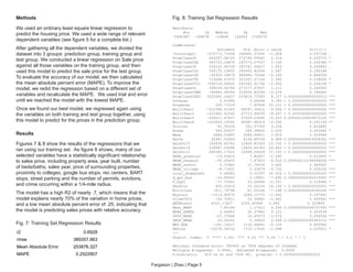
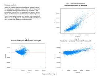
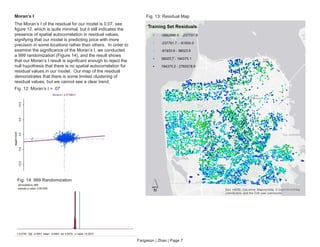
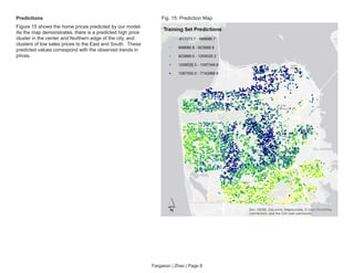
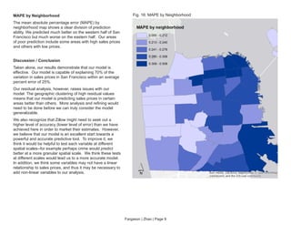
This document summarizes a hedonic home price prediction model developed by Phil Fargason and Jianting Zhao for Zillow. They collected 23 variables related to home characteristics, location, neighborhood attributes, crime, transportation and demographics. Their linear regression model explained 70% of variation in home prices in San Francisco with a mean absolute percentage error of 25%. Key factors correlated with higher prices included property size, number of bedrooms/bathrooms, proximity to transit and colleges, and surrounding home prices.

1. Fargason | Zhao | Page 1
CPLN 590
Midterm Project
Hedonic Home-Price Prediction
Phil Fargason | Jianting Zhao
11/10/2016

2. Fargason | Zhao | Page 2
Introduction
This report describes our process for developing a hedonic
price model to predict home sales in San Francisco. Home
prices in San Francisco are volatile and vary widely across
home types and geographic areas, as you can see clearly
in figure 1 at right. To help our client, Zillow, better predict
the variability in price, we developed a regression model that
accounts for a wide variety in relevant variables. We believe
that fluctuations in home prices are complex phenomena,
resulting from the inter-relationship of many different factors.
This complexity makes a perfect prediction impossible. We
sought to get as close as possible to an accurate prediction
by including a wide range of relevant variables related to
the economic, social, transportation, safety, housing, and
environmental characteristics surrounding each home. Our
overall strategy was to include a breadth of factors, each of
which relate to home prices.
The model that we have developed explains roughly 70%
of the variation in home prices in San Francisco (R2 of
.69) within a 25% range of accuracy for each price that
we predict (MAPE of .25). Our model shows a regularly
distributed residual, both numerically and geographically,
meaning that our model is generalizable--equally able to
predict sales price in one neighborhood versus another. All
of these factors lead us to believe that our model will be
useful for Zillow.
Data
To complete our analysis we gathered 23 variables from San
Francisco’s open data site in addition to the home details
found in our original dataset (see figure 5 for a complete
list). We attributed these data to our home prices using four
techniques:
1. For already aggregated data, such as demographic
data, we attributed data to each point according to
the census tract in which it falls.
2. For data related to relatively sparse resources/
occurrences (parks, transit-stations, schools) we
measured the distance from each home to the
nearest occurrence.
Fig. 1: Sales Prices 2012-2015
Fig. 2: Google Bus Locations
Sales Prices 2012-2015 ($)
0 - 585,001
585,002 - 790,001
790,002 - 1,020,003
1,020,004 - 1,475,003
1,475,004 - 4,750,003
[ 1
Miles 1:75,000
Data Source: City of San Francisco
Google Shuttles
[ 1
Miles 1:75,000
Data Source: Google

3. Fargason | Zhao | Page 3
Crime Incidents 2015
0
Low
High
[ 1
Miles 1:76,828
Data Source: City of San Francisco
Kernel Density Used for this Map
Buyouts of Rent Stabilized Apartments
0
Low Density
High Density
[ 1
Miles 1:75,000
Data Source: City of San Francisco
Map uses Kernel Density
Fig. 3: Crime Incidents 2015
Fig. 4: Buyouts of Rent Stabilized Apartments
3. For relatively common occurrences (permits, crimes,
evictions) we measured the number of occurrences
within a 1/4-mile area of the subject property.
4. In order to measure spatial-autocorrelation (the
amount that one sale price is determined by
neighboring sale prices) we took the average sale
price of the 7 properties nearest to the subject
property.
Much of the data we selected also showed clusters in space.
For example, Google Shuttle stops (figure 2) tend to cluster
in the Mission/Dolores districts, an area with many high
home prices in central San Francisco, as well as around
the central business district. These areas both tend to have
a high prevalence of buyouts of rent stabilized apartments
(figure 4.) While the CBD tends to show large levels of
crime, Mission/Dolores show lower levels.
When testing the correlation of our variables (see figure 6
on the following page) we saw that only a few variables had
strong correlations with sales prices. The strongest positive
correlations that we found were our spatial auto-correlation
variable (local area average sales price), the property area,
number of beds/baths, and building permit activity. Smaller
positive effects included evictions, buyouts, and percent
white. A few variables had strong negative correlations,
including the distance to google shuttles (meaning stations
are associated with higher sales price.) To a lesser extent,
household size, percent hispanic, and on street parking all
had a negative relationship to sales price.

4. Fargason | Zhao | Page 4
Regression Analysis for Willingness to Pay for Transit
Statistic Mean St. Dev. Min Max
Sales Price 1065593.0 736123.6 0.0 4750003.0
Lot Area 246118.5 137279.6 0.0 1890500.0
Property Area 1635.7 783.9 0.0 24308.0
Year Built 1.3 0.5 1.0 4.0
Stories 1.5 11.9 0.0 829.0
Rooms 6.3 13.6 0.0 1353.0
Beds 1.7 1.7 0.0 20.0
Baths 1.8 1.0 0.0 25.0
Sale Year 13.4 1.1 12.0 15.0
Distance to Green Connection 811.6 619.2 20.7 3447.3
Distance to Recreation Area 867.0 606.5 0.0 3820.0
Distance to School 1577.7 482.0 286.6 4208.7
Distance to College 5456.6 2998.4 74.3 15963.1
Median Age 40.4 4.1 0.0 70.4
Population Density 78077817.0 33819154.0 889976.3 377907004.0
Percent Black 0.1 0.1 0.0 0.6
Percent Hispanic 0.1 0.1 0.0 0.6
Household Size 2.7 0.7 0.0 4.2
Percent Vacant 0.1 0.0 0.0 0.4
Local Area Average Sales Price 1068294.0 541017.3 104001.4 4283002.0
Distance to Google Bus Stop 4712.5 3114.5 80.0 15160.0
Building Permits Issued 638.6 438.9 25.0 2968.0
Evictions 164.7 125.2 0.0 1411.0
Buyouts 6.7 7.0 0.0 48.0
Crime 2015 479.6 490.6 12.0 9157.0
Affordable Housing 0.6 1.6 0.0 37.0
Distance to BART 8650.8 5741.4 256.0 26536.0
Distance to SFMTA 382.7 226.1 24.0 1517.0
Off Street Parking 1255.2 534.2 127.6 4410.1
On Street Parking 1632.4 1160.6 46.3 6227.4
Percent White 0.5 0.2 0.1 0.9
Summary Statistics
Fig. 6: Correlation MatrixFig. 5: Summary Statistics

5. Fargason | Zhao | Page 5
Methods
We used an ordinary least square linear regression to
predict the housing price. We used a wide range of relevant
dependent variables (see figure 5 for a complete list.)
After gathering all the dependent variables, we divided the
dataset into 3 groups: prediction group, training group and
test group. We conducted a linear regression on Sale price
against all those variables on the training group, and then
used this model to predict the sale price for the test group.
To evaluate the accuracy of our model, we then calculated
the mean absolute percent error (MAPE). To improve the
model, we redid the regression based on a different set of
variables and recalculate the MAPE. We used trial and error
until we reached the model with the lowest MAPE.
Once we found our best model, we regressed again using
the variables on both training and test group together, using
this model to predict for the prices in the prediction group.
Results
Figures 7 & 8 show the results of the regressions that we
ran using our training set. As figure 8 shows, many of our
selected variables have a statistically significant relationship
to sales price, including property area, year built, number
of beds/baths, sales year, price of surrounding properties,
proximity to colleges, google bus stops, rec centers, BART
stops, street parking and the number of permits, evictions,
and crime occurring within a 1/4-mile radius.
The model has a high R2 of nearly .7, which means that the
model explains nearly 70% of the variation in home prices,
and a low mean absolute percent error of .25, indicating that
the model is predicting sales prices with relative accuracy.
Residuals:
Min 1Q Median 3Q Max
-5892987 -189678 -24848 146520 2760579
Coefficients:
Estimate Std. Error t value Pr(>|t|)
(Intercept) -475773.73008 286900.37656 -1.658 0.097294 .
PropClassCD 640297.94125 276749.59942 2.314 0.020715 *
PropClassCDA 643723.29878 297273.07537 2.165 0.030386 *
PropClassCF 554125.90728 283761.59427 1.953 0.050882 .
PropClassCLZ 305170.10855 291600.42056 1.047 0.295348
PropClassCOZ -93309.39479 480580.72268 -0.194 0.846056
PropClassCTH 712698.47075 301207.37106 2.366 0.018000 *
PropClassCTIC -593718.56930 283343.91736 -2.095 0.036169 *
PropClassCZ 308154.54784 277277.57837 1.111 0.266450
PropClassCZBM -84945.98354 310004.83294 -0.274 0.784081
PropClassCZEU 3525492.24427 433819.72083 8.127 0.000000000000000512 ***
LotArea 0.43949 0.04494 9.780 < 0.0000000000000002 ***
PropArea 250.77219 7.80958 32.111 < 0.0000000000000002 ***
BuiltYear1 -422368.51083 46597.35612 -9.064 < 0.0000000000000002 ***
BuiltYear2 -431662.42550 47713.99359 -9.047 < 0.0000000000000002 ***
BuiltYear3 -306211.47637 57524.23490 -5.323 0.000000104924875130 ***
BuiltYear4 -203429.19340 62587.98314 -3.250 0.001158 **
Stories 82.55209 352.57350 0.234 0.814882
Rooms 584.50637 289.38856 2.020 0.043440 *
Beds 2684.01897 3289.64811 0.816 0.414584
Baths 42947.00904 6144.86754 6.989 0.000000000003004362 ***
SaleYr13 162838.60763 12428.82524 13.102 < 0.0000000000000002 ***
SaleYr14 318987.23088 12829.84783 24.863 < 0.0000000000000002 ***
SaleYr15 490380.17022 12999.54929 37.723 < 0.0000000000000002 ***
NEAR_greencon -19.43616 7.80607 -2.490 0.012800 *
NEAR_recpark -35.65455 7.87823 -4.526 0.000006112198956638 ***
NEAR_school 0.72962 11.76376 0.062 0.950547
NEAR_college -8.71831 2.33679 -3.731 0.000192 ***
Local_AvgSalePr 0.46065 0.01297 35.524 < 0.0000000000000002 ***
d_ggl_bus -16.84920 2.18951 -7.695 0.000000000000015905 ***
P_Sqft -77.75561 33.26996 -2.337 0.019460 *
Permits 655.32614 25.05234 26.158 < 0.0000000000000002 ***
Evictions -611.79798 81.05246 -7.548 0.000000000000049340 ***
Buyouts -1113.92479 1069.12772 -1.042 0.297491
Crime2015 -56.72811 16.39082 -3.461 0.000541 ***
AfffHousin 4220.17427 4250.82468 0.993 0.320845
Near_BART 7.45164 1.17612 6.336 0.000000000249757350 ***
NEAR_SFMTA 2.46963 20.37682 0.121 0.903538
OFSP_NEAR -37.37848 10.45973 -3.574 0.000354 ***
ONSP_NEAR 24.54355 5.34830 4.589 0.000004525395943112 ***
MED.AGE -141.14017 1133.96641 -0.124 0.900950
HHSize -16178.34510 7710.17630 -2.098 0.035911 *
---
Signif. codes: 0 ‘***’ 0.001 ‘**’ 0.01 ‘*’ 0.05 ‘.’ 0.1 ‘ ’ 1
Residual standard error: 390400 on 7504 degrees of freedom
Multiple R-squared: 0.6945, Adjusted R-squared: 0.6928
F-statistic: 416 on 41 and 7504 DF, p-value: < 0.00000000000000022
Fig. 8: Training Set Regression Results
Fig. 7: Training Set Regression Results
r2 0.6928
rmse 389357.863
Mean Absolute Error 253876.327
MAPE 0.2522907

6. Fargason | Zhao | Page 6
Fig. 9: Cross-Validation Results
Fig. 11Fig. 10
Residual Analysis
When we mapped our predictions for the test set against
the actual observed sales prices in this set, we found that
our error was evenly distributed around the mean. Our
predictions differed from the observed in a random fashion
(figure 9) when we conducted our cross-validation process.
When mapping the residual as a function of predicted and
observed values (figures 10 & 11) we found that for the most
part, the residuals were randomly distributed.

7. Fargason | Zhao | Page 7
Moran’s I
The Moran’s I of the residual for our model is 0.07, see
figure 12, which is quite minimal, but it still indicates the
presence of spatial autocorrelation in residual values,
signifying that our model is predicting price with more
precision in some locations rather than others. In order to
examine the significance of the Moran’s I, we conducted
a 999 randomization (Figure 14), and the result shows
that our Moran’s I result is significant enough to reject the
null hypothesis that there is no spatial autocorrelation for
residual values in our model. Our map of the residual
demonstrates that there is some limited clustering of
residual values, but we cannot see a clear trend.
Fig. 12: Moran’s I = .07
Fig. 13: Residual Map
Fig. 14: 999 Randomization

8. Fargason | Zhao | Page 8
Fig. 15: Prediction MapPredictions
Figure 15 shows the home prices predicted by our model.
As the map demonstrates, there is a predicted high price
cluster in the center and Northern edge of the city, and
clusters of low sales prices to the East and South. These
predicted values correspond with the observed trends in
prices.

9. Fargason | Zhao | Page 9
MAPE by Neighborhood
The mean absolute percentage error (MAPE) by
neighborhood map shows a clear division of prediction
ability. We predicted much better on the western half of San
Francisco but much worse on the eastern half. Our areas
of poor prediction include some areas with high sales prices
and others with low prices.
Discussion / Conclusion
Taken alone, our results demonstrate that our model is
effective. Our model is capable of explaining 70% of the
variation in sales prices in San Francisco within an average
percent error of 25%.
Our residual analysis, however, raises issues with our
model. The geographic clustering of high residual values
means that our model is predicting sales prices in certain
areas better than others. More analysis and refining would
need to be done before we can truly consider the model
generalizable.
We also recognize that Zillow might need to seek out a
higher level of accuracy (lower level of error) than we have
achieved here in order to market their estimates. However,
we believe that our model is an excellent start towards a
powerful and accurate predictive tool. To improve it, we
think it would be helpful to test each variable at different
spatial scales--for example perhaps crime would predict
better at a more granular spatial scale. We think these tests
at different scales would lead us to a more accurate model.
In addition, we think some variables may not have a linear
relationship to sales prices, and thus it may be necessary to
add non-linear variables to our analysis.
Fig. 16: MAPE by Neighborhood