Sol3
•
0 likes•119 views

1) The balancing of a pencil is modeled as an exponential decay process with time constant τ = m/g, where m is the pencil's mass and g is gravity. 2) Solving the differential equation governing the pencil's angular displacement θ(t) shows that θ(t) grows exponentially until it reaches 1 radian, at which point the balancing time t is found. 3) For typical parameter values of m = 0.01 kg and length = 0.1 m, the calculated balancing time is approximately 3.5 seconds. Remarkably, this everyday time scale results from the combination of quantum effects and exponential growth.

Recommended
More Related Content
What's hot
What's hot (18)
Similar to Sol3
Similar to Sol3 (20)
More from eli priyatna laidan
More from eli priyatna laidan (20)
Sol3
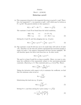
- 1. Solution Week 3 (9/30/02) Balancing a pencil (a) The component of gravity in the tangential direction is mg sin θ ≈ mgθ. There- fore, the tangential F = ma equation is mgθ = m ¨θ, which may be written as ¨θ = (g/ )θ. The general solution to this equation is θ(t) = Aet/τ + Be−t/τ , where τ ≡ /g. (1) The constants A and B are found from the initial conditions, θ(0) = θ0 =⇒ A + B = θ0, ˙θ(0) = ω0 =⇒ (A − B)/τ = ω0. (2) Solving for A and B, and then plugging into eq. (1) gives θ(t) = 1 2 (θ0 + ω0τ) et/τ + 1 2 (θ0 − ω0τ) e−t/τ . (3) (b) The constants A and B will turn out to be small (they will each be of order√ ¯h). Therefore, by the time the positive exponential has increased enough to make θ of order 1, the negative exponential will have become negligible. We will therefore ignore the latter term from here on. In other words, θ(t) ≈ 1 2 (θ0 + ω0τ) et/τ . (4) The goal is to keep θ small for as long as possible. Hence, we want to min- imize the coefficient of the exponential, subject to the uncertainty-principle constraint, ( θ0)(m ω0) ≥ ¯h. This constraint gives ω0 ≥ ¯h/(m 2θ0). Hence, θ(t) ≥ 1 2 θ0 + ¯hτ m 2θ0 et/τ . (5) Taking the derivative with respect to θ0 to minimize the coefficient, we find that the minimum value occurs at θ0 = ¯hτ m 2 . (6) Substituting this back into eq. (5) gives θ(t) ≥ ¯hτ m 2 et/τ . (7) Setting θ ≈ 1, and then solving for t gives (using τ ≡ /g) t ≤ 1 4 g ln m2 3g ¯h2 . (8)
- 2. With the given values, m = 0.01 kg and = 0.1 m, along with g = 10 m/s2 and ¯h = 1.06 · 10−34 Js, we obtain t ≤ 1 4 (0.1 s) ln(9 · 1061 ) ≈ 3.5 s. (9) No matter how clever you are, and no matter how much money you spend on the newest, cutting-edge pencil-balancing equipment, you can never get a pencil to balance for more than about four seconds. Remarks: This smallness of this answer is quite amazing. It is remarkable that a quantum effect on a macroscopic object can produce an everyday value for a time scale. Basically, the point here is that the fast exponential growth of θ (which gives rise to the log in the final result for t) wins out over the smallness of ¯h, and produces a result for t of order 1. When push comes to shove, exponential effects always win. The above value for t depends strongly on and g, through the /g term. But the dependence on m, , and g in the log term is very weak. If m were increased by a factor of 1000, for example, the result for t would increase by only about 10%. Note that this implies that any factors of order 1 that we neglected throughout this problem are completely irrelevant. They will appear in the argument of the log term, and will thus have negligible effect. Note that dimensional analysis, which is generally a very powerful tool, won’t get you too far in this problem. The quantity /g has dimensions of time, and the quantity η ≡ m2 3 g/¯h2 is dimensionless (it is the only such quantity), so the balancing time must take the form t ≈ g f(η), (10) where f is some function. If the leading term in f were a power (even, for example, a square root), then t would essentially be infinite (t ≈ 1030 s for the square root). But f in fact turns out to be a log (which you can’t determine without solving the problem), which completely cancels out the smallness of ¯h, reducing an essentially infinite time down to a few seconds.