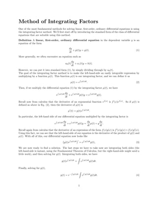
SlideShare a Scribd company logo
1 of 2
Download to read offline
Method of Integrating Factors
One of the most fundamental methods for solving linear, first-order, ordinary differential equations is using
the integrating factor method. We’ll first start off by introducing the standard form of the class of differential
equations that are solvable using this method.
Definition A linear, first-order, ordinary differential equation in the dependent variable y is an
equation of the form
dy
dt
+ p(t)y = g(t). (1)
More generally, we often encounter an equation such as
a0(t)
dy
dt
+ a1(t)y = h(t).
However, we can put it into standard form (1), by simply dividing through by a0(t).
The goal of the integrating factor method is to make the left-hand-side an easily integrable expression by
multiplying by a function µ(t). This function µ(t) is our integrating factor, and we can define it as
µ(t) = e p(t)dt
. (2)
Then, if we multiply the differential equation (1) by the integrating factor µ(t), we have
e p(t)dt dy
dt
+ e p(t)dt
p(t)y = e p(t)dt
g(t).
Recall now from calculus that the derivative of an exponential function ef(x)
is f (x)ef(x)
. So if µ(t) is
defined as above in Eq. (2), then the derivative of µ(t) is
µ (t) = p(t)e p(t)dt
.
In particular, the left-hand side of our differential equation multiplied by the integrating factor is
e p(t)dt dy
dt
+ e p(t)dt
p(t)y =
dy
dt
µ(t) + y
dµ
dt
.
Recall again from calculus that the derivative of an expression of the form f(x)g(x) is f (x)g(x)+f(x)g (x).
Using this fact, we can see that the left-hand-side of our equation is the derivative of the product of y(t) and
µ(t). With all of this, our differential equation now looks like
y(t)e p(t)dt
= e p(t)dt
g(t), (3)
We are now ready to find a solution. The last steps we have to take now are integrating both sides (the
left-hand-side is instant, using the Fundamental Theorem of Calculus, but the right-hand-side might need a
little work), and then solving for y(t). Integrating both sides, we have
y(t)e p(t)dt
= e p(t)dt
g(t)dt.
Finally, solving for y(t),
y(t) = e− p(t)dt
e p(t)dt
g(t)dt. (4)
1
And we are done! Outlined below is the algorithm for solving linear, first-order, ordinary differential equa-
tions with the integrating factor method.
To Solve an ODE with the Integrating Factor Method:
1. Put the equation in standard form such as in Eq. (1).
2. Calculate the integrating factor µ(t) using the definition in Eq. (2).
3. Multiply the differential equation by µ(t) and write it as written in Eq. (3).
4. Integrate both sides of the differential equation.
5. Solve for y(t) to obtain a general solution.
2

More Related Content

What's hot

Polynomial Functions
Polynomial FunctionsPolynomial Functions
Polynomial Functions
nicole379865
 
3 2 Polynomial Functions And Their Graphs
3 2 Polynomial Functions And Their Graphs3 2 Polynomial Functions And Their Graphs
3 2 Polynomial Functions And Their Graphs
silvia
 
Integration ftw cyrus
Integration ftw cyrusIntegration ftw cyrus
Integration ftw cyrus
canalculus
 
Linear Functions
Linear FunctionsLinear Functions
Linear Functions
kliegey524
 
Linear functions and modeling
Linear functions and modelingLinear functions and modeling
Linear functions and modeling
IVY SOLIS
 
Linear Equations Ppt
Linear Equations PptLinear Equations Ppt
Linear Equations Ppt
Scott R
 
 Igcse mathematics additional standards
 Igcse   mathematics additional standards Igcse   mathematics additional standards
 Igcse mathematics additional standards
Ross
 
Polynomial and thier graphs
Polynomial and thier graphsPolynomial and thier graphs
Polynomial and thier graphs
Jessica Garcia
 

What's hot (20)

Polynomial Functions
Polynomial FunctionsPolynomial Functions
Polynomial Functions
 
8.2 Equations W Two Variables
8.2 Equations W Two Variables8.2 Equations W Two Variables
8.2 Equations W Two Variables
 
The International Journal of Engineering and Science (The IJES)
The International Journal of Engineering and Science (The IJES)The International Journal of Engineering and Science (The IJES)
The International Journal of Engineering and Science (The IJES)
 
Graphs of trigonometric exponential functions lecture
Graphs of trigonometric exponential functions lectureGraphs of trigonometric exponential functions lecture
Graphs of trigonometric exponential functions lecture
 
Larson 4.3
Larson 4.3Larson 4.3
Larson 4.3
 
3 2 Polynomial Functions And Their Graphs
3 2 Polynomial Functions And Their Graphs3 2 Polynomial Functions And Their Graphs
3 2 Polynomial Functions And Their Graphs
 
Linear functions
Linear functions Linear functions
Linear functions
 
Slop lecture
Slop lectureSlop lecture
Slop lecture
 
Paso 3 profundizar y contextualizar el conocimiento de la unidad 2
Paso 3  profundizar y contextualizar el conocimiento de la unidad 2Paso 3  profundizar y contextualizar el conocimiento de la unidad 2
Paso 3 profundizar y contextualizar el conocimiento de la unidad 2
 
Integration ftw cyrus
Integration ftw cyrusIntegration ftw cyrus
Integration ftw cyrus
 
Linear Functions
Linear FunctionsLinear Functions
Linear Functions
 
Linear functions and modeling
Linear functions and modelingLinear functions and modeling
Linear functions and modeling
 
Kelompok 6
Kelompok 6Kelompok 6
Kelompok 6
 
Linear Equations Ppt
Linear Equations PptLinear Equations Ppt
Linear Equations Ppt
 
Polynomials lecture
Polynomials lecturePolynomials lecture
Polynomials lecture
 
 Igcse mathematics additional standards
 Igcse   mathematics additional standards Igcse   mathematics additional standards
 Igcse mathematics additional standards
 
Analisis unidad 3
Analisis unidad 3Analisis unidad 3
Analisis unidad 3
 
Limits of a Function
Limits of a FunctionLimits of a Function
Limits of a Function
 
Polynomial and thier graphs
Polynomial and thier graphsPolynomial and thier graphs
Polynomial and thier graphs
 
Introduction to Functions
Introduction to FunctionsIntroduction to Functions
Introduction to Functions
 

Similar to Integrating_Factors

torsionbinormalnotes
torsionbinormalnotestorsionbinormalnotes
torsionbinormalnotes
Jeremy Lane
 
X01 Supervised learning problem linear regression one feature theorie
X01 Supervised learning problem linear regression one feature theorieX01 Supervised learning problem linear regression one feature theorie
X01 Supervised learning problem linear regression one feature theorie
Marco Moldenhauer
 
Laplace transform
Laplace transformLaplace transform
Laplace transform
joni joy
 
On problem-of-parameters-identification-of-dynamic-object
On problem-of-parameters-identification-of-dynamic-objectOn problem-of-parameters-identification-of-dynamic-object
On problem-of-parameters-identification-of-dynamic-object
Cemal Ardil
 

Similar to Integrating_Factors (20)

Ch07 7
Ch07 7Ch07 7
Ch07 7
 
A Solution Manual And Notes For Kalman Filtering Theory And Practice Using ...
A Solution Manual And Notes For  Kalman Filtering  Theory And Practice Using ...A Solution Manual And Notes For  Kalman Filtering  Theory And Practice Using ...
A Solution Manual And Notes For Kalman Filtering Theory And Practice Using ...
 
torsionbinormalnotes
torsionbinormalnotestorsionbinormalnotes
torsionbinormalnotes
 
Differential Equations Lecture: Non-Homogeneous Linear Differential Equations
Differential Equations Lecture: Non-Homogeneous Linear Differential EquationsDifferential Equations Lecture: Non-Homogeneous Linear Differential Equations
Differential Equations Lecture: Non-Homogeneous Linear Differential Equations
 
Tutorial on EM algorithm – Part 2
Tutorial on EM algorithm – Part 2Tutorial on EM algorithm – Part 2
Tutorial on EM algorithm – Part 2
 
NONLINEAR DIFFERENCE EQUATIONS WITH SMALL PARAMETERS OF MULTIPLE SCALES
NONLINEAR DIFFERENCE EQUATIONS WITH SMALL PARAMETERS OF MULTIPLE SCALESNONLINEAR DIFFERENCE EQUATIONS WITH SMALL PARAMETERS OF MULTIPLE SCALES
NONLINEAR DIFFERENCE EQUATIONS WITH SMALL PARAMETERS OF MULTIPLE SCALES
 
International Journal of Mathematics and Statistics Invention (IJMSI)
International Journal of Mathematics and Statistics Invention (IJMSI) International Journal of Mathematics and Statistics Invention (IJMSI)
International Journal of Mathematics and Statistics Invention (IJMSI)
 
X01 Supervised learning problem linear regression one feature theorie
X01 Supervised learning problem linear regression one feature theorieX01 Supervised learning problem linear regression one feature theorie
X01 Supervised learning problem linear regression one feature theorie
 
Linear regression
Linear regressionLinear regression
Linear regression
 
Ch02 1
Ch02 1Ch02 1
Ch02 1
 
An Approach For Solving Nonlinear Programming Problems
An Approach For Solving Nonlinear Programming ProblemsAn Approach For Solving Nonlinear Programming Problems
An Approach For Solving Nonlinear Programming Problems
 
microproject@math (1).pdf
microproject@math (1).pdfmicroproject@math (1).pdf
microproject@math (1).pdf
 
Free Ebooks Download
Free Ebooks Download Free Ebooks Download
Free Ebooks Download
 
Signal Processing Homework Help
Signal Processing Homework HelpSignal Processing Homework Help
Signal Processing Homework Help
 
Laplace transform
Laplace transformLaplace transform
Laplace transform
 
Week 7
Week 7Week 7
Week 7
 
Ma2002 1.19 rm
Ma2002 1.19 rmMa2002 1.19 rm
Ma2002 1.19 rm
 
On problem-of-parameters-identification-of-dynamic-object
On problem-of-parameters-identification-of-dynamic-objectOn problem-of-parameters-identification-of-dynamic-object
On problem-of-parameters-identification-of-dynamic-object
 
D021018022
D021018022D021018022
D021018022
 
Lec17
Lec17Lec17
Lec17
 

Integrating_Factors

  • 1. Method of Integrating Factors One of the most fundamental methods for solving linear, first-order, ordinary differential equations is using the integrating factor method. We’ll first start off by introducing the standard form of the class of differential equations that are solvable using this method. Definition A linear, first-order, ordinary differential equation in the dependent variable y is an equation of the form dy dt + p(t)y = g(t). (1) More generally, we often encounter an equation such as a0(t) dy dt + a1(t)y = h(t). However, we can put it into standard form (1), by simply dividing through by a0(t). The goal of the integrating factor method is to make the left-hand-side an easily integrable expression by multiplying by a function µ(t). This function µ(t) is our integrating factor, and we can define it as µ(t) = e p(t)dt . (2) Then, if we multiply the differential equation (1) by the integrating factor µ(t), we have e p(t)dt dy dt + e p(t)dt p(t)y = e p(t)dt g(t). Recall now from calculus that the derivative of an exponential function ef(x) is f (x)ef(x) . So if µ(t) is defined as above in Eq. (2), then the derivative of µ(t) is µ (t) = p(t)e p(t)dt . In particular, the left-hand side of our differential equation multiplied by the integrating factor is e p(t)dt dy dt + e p(t)dt p(t)y = dy dt µ(t) + y dµ dt . Recall again from calculus that the derivative of an expression of the form f(x)g(x) is f (x)g(x)+f(x)g (x). Using this fact, we can see that the left-hand-side of our equation is the derivative of the product of y(t) and µ(t). With all of this, our differential equation now looks like y(t)e p(t)dt = e p(t)dt g(t), (3) We are now ready to find a solution. The last steps we have to take now are integrating both sides (the left-hand-side is instant, using the Fundamental Theorem of Calculus, but the right-hand-side might need a little work), and then solving for y(t). Integrating both sides, we have y(t)e p(t)dt = e p(t)dt g(t)dt. Finally, solving for y(t), y(t) = e− p(t)dt e p(t)dt g(t)dt. (4) 1
  • 2. And we are done! Outlined below is the algorithm for solving linear, first-order, ordinary differential equa- tions with the integrating factor method. To Solve an ODE with the Integrating Factor Method: 1. Put the equation in standard form such as in Eq. (1). 2. Calculate the integrating factor µ(t) using the definition in Eq. (2). 3. Multiply the differential equation by µ(t) and write it as written in Eq. (3). 4. Integrate both sides of the differential equation. 5. Solve for y(t) to obtain a general solution. 2