This document discusses soil shear strength, focusing on fine-grained soils. It covers topics like clay mineralogy, bonding mechanisms, structural units of common clay minerals like kaolinite and montmorillonite, double layer water, intergranular pressure, water pressure, the relationship between mineralogy and shear strength, soil fabric, Atterberg limits, ideal soil laboratory testing, and undisturbed Shelby tube sampling. 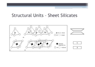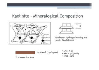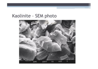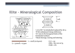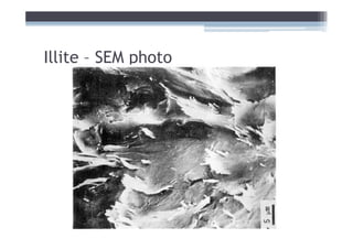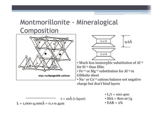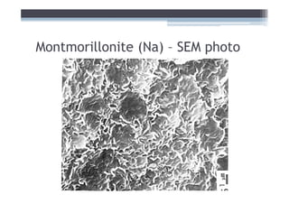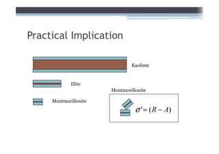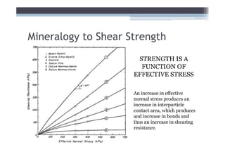In summary: 1) It describes the mineralogical composition and structure of common clay minerals and how they influence shear strength. 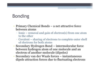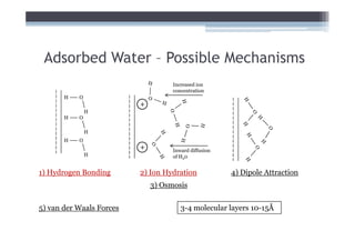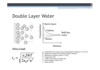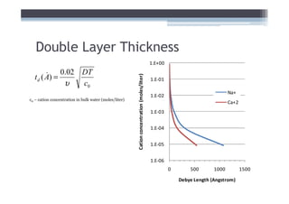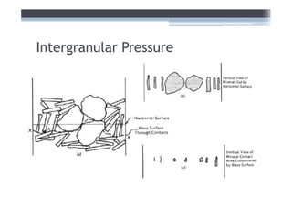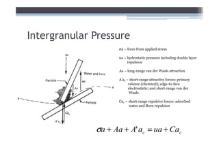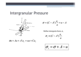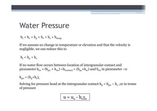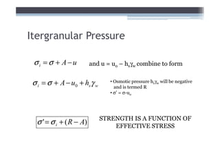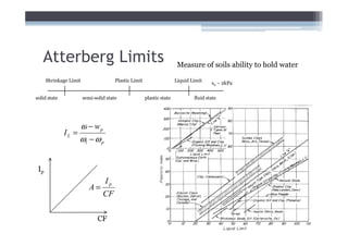2) It explains concepts like double layer water, intergranular pressure, and how water pressure relates to shear strength. 3) There is a relationship

1. ADVANCED SOIL SHEAR
STRENGTH – Fine-grained Soils
Donald C. Wotring, Ph.D., P.E.
December 2008

2. CLAY MINERALOGY

3. Bonding
• Primary Chemical Bonds – a net attractive force
between atoms
▫ Ionic – removal and gain of electron(s) from one atom
to the other
▫ Covalent – sharing of electrons to complete outer shell
of electrons for both atoms
• Secondary Hydrogen Bond – intermolecular force
between hydrogen atom of one molecule and an
electron of another molecule (dipoles)
• Secondary van der Waals forces – instantaneous
dipole attraction forces due to fluctuating electrons

4. Structural Units – Sheet Silicates
G
B

5. Kaolinite – Mineralogical Composition
G
7Å
G
Interlayer - Hydrogen bonding and
van der Waals forces
• L/t = 5-10
t = 1000Å (140 layers)
• SSA = 5-15 m2/g
• EAR = 12%
L = 10,000Å = 1µm

6. Kaolinite – SEM photo

7. Illite - Mineralogical Composition
G or B 10Å
G or B
• 1/6 of Si+4 in tetrahedral replaced by Al+3
Net unbalanced charge deficiency
• K+ ions in the hexagonal holes of the
tetrahedral surfaces
• Basal cleavage, tearing and tattering
t = 100Å (10 layers) • L/t = 30
L = 3,000Å = 0.3µm • SSA = 80-100 m2/g
• EAR = 6%

8. Illite – SEM photo

9. Montmorillonite - Mineralogical
Composition
G or B 9.6Å
G or B
• Much less isomorphic substitution of Al+3
for Si+4 than Illite
• Fe+2 or Mg+2 substitution for Al+3 in
Gibbsite sheet
• Na+ or Ca+2 cations balance net negative
charge but don’t bind layers
• L/t = 100-400
t = 10Å (1 layer) • SSA = 800 m2/g
L = 1,000-4,000Å = 0.1-0.4µm • EAR = 2%

10. Montmorillonite (Na) – SEM photo

11. Adsorbed Water – Possible Mechanisms
Increased ion
concentration
H O
+
H
H O
H
H O
+ Inward diffusion
H of H20
1) Hydrogen Bonding 2) Ion Hydration 4) Dipole Attraction
3) Osmosis
5) van der Waals Forces 3-4 molecular layers 10-15Å

12. Double Layer Water
+ - Stern’s layer
Concentration
+ - +
+ + +
- - - Cations
+ + - Bulk free
-
+ - + - water
+ + +
- Anions
-
+ + - -
Distance
Debye Length
ε0 – permittivity of a vacuum (ease of polarization) (8.854x10-12 C2/J*m)
ε 0DkT
D – Dielectric constant (force between electric charges)
k – Boltzmann constant (1.38x10-23 J/oK)
td = T – temperature (oK)
2n0 e υ
n0 – bulk concentration (number/m3)
2 2 e – electric charge (1.60x10-19 C)
v – cation valence

13. Double Layer Thickness
1.E+00
0.02 DT
t d ( A) =
&
Cation concentration (moles/liter)
υ
1.E-01
c0
Na+
1.E-02
c0 – cation concentration in bulk water (moles/liter)
Ca+2
1.E-03
1.E-04
1.E-05
1.E-06
0 500 1000 1500
Debye Length (Angstrom)

14. Intergranular Pressure

15. Intergranular Pressure
σa – force from applied stress
ua – hydrostatic pressure including double layer
repulsion
Aa – long-range van der Waals attraction
A’ac – short-range attractive forces: primary
valence (chemical); edge-to-face
electrostatic; and short-range van der
Waals.
Cac – short-range repulsive forces: adsorbed
water and Born repulsion
σa + Aa + A' ac = ua + Cac

16. Intergranular Pressure
ac
σ = (C − A' ) + u − A
a
Define intergrain force, σi
ac
σ i ≡ (C − A' )
a
σa + Aa + A' ac = ua + Cac
σi = σ + A−u

17. Water Pressure
ht = he + hp + hv + hs + htemp
If we assume no change in temperature or elevation and that the velocity is
negligible, we can reduce this to
ht = hp + hs
If no water flow occurs between location of intergranular contact and
piezometer ht0 = (hp0 + hs0) =htcontact = (hpc+hsc) and hs0 in piezometer ~0
hp0 = (hp+hs)c
Solving for pressure head at the intergranular contact hp = hp0 – hs ,or in terms
of pressure
u = uo - hsγw

18. Itergranular Pressure
σi = σ + A −u and u = uo – hsγw combine to form
σ i = σ + A − u0 + hsγ w • Osmotic pressure hsγw will be negative
and is termed R
• σ’ = σ-uo
STRENGTH IS A FUNCTION OF
σ ' = σ i + ( R − A) EFFECTIVE STRESS

19. Practical Implication
Kaolinte
Illite
Montmorillonite
Montmorillonite
σ ' = ( R − A)

20. Mineralogy to Shear Strength
STRENGTH IS A
FUNCTION OF
EFFECTIVE STRESS
An increase in effective
normal stress produces an
increase in interparticle
contact area, which produces
and increase in bonds and
thus an increase in shearing
resistance.

21. Soil Fabric
Orientation of N ature of Particles
Particles
Dispersed Flocculated (Aggregated)
Random
Highly Oriented

22. Atterberg Limits Measure of soils ability to hold water
Shrinkage Limit Plastic Limit Liquid Limit su ~ 2kPa
solid state semi-solid state plastic state fluid state
ω − wp
IL =
ωl − ω p
Ip
Ip
A=
CF
CF

23. SOIL SAMPLING

24. Ideal Soil Laboratory Testing Criteria
• High quality samples with minimum
disturbance
• Reconsolidation to in-situ stress (K0)
• Account for mode of shear
▫ Intermediate principal stress
▫ Direction of applied major principal stress at
failure
• Test at strain rate approaching field conditions
• Strain compatibility

25. “Undisturbed” Shelby Tube Sampling
Total, σ = Neutral, u + Effective, σ’
0 Residual (capillarity)
pressure, after sampling
σ’vo = ur
−ur
0 σ’ho = ur

26. Minimize Sampling Disturbance
γm zw  2s  γ z 
= 1− +
 K 0 − u ( E )  b + w 
γw z  σ 'v 0  γ w z 
 
Drilling (A-B) - Use appropriate drilling mud
If OCR Soil:
 su ( E )   su ( E ) 

σ'   =
  (OCR )0.8

 v 0 OCR  σ 'v 0  NC
(K 0 )OCR = K 0 p (OCR )(1− K 0p)

27. Minimize Sampling Disturbance
Tube Sampling and Extraction (C-D)
• Fixed piston sampler (standard in NE)
• Min. outside diameter (76 mm)
• D0/t >45
• Insert tube, allow setup (20 min),
slowly rotate, and slowly withdraw
• Radiography
• Germaine (2003) tube extrusion
• Prepare samples in a humid room
• Moist stones

28. Reconsolidate to In-Situ Stress
Conditions
Volumetric strain kept to between
1.5% and 4% at σ’v0
Volumetric SQD
Strain (%)
<1 A
1-2 B
2-4 C
4-8 D
>8 E

29. Modes of Shear and Strain
Compatibility
σ'1f
TC TE
σ'1f
σ'1f
DSS
s(PSC) ~ 1.1 s(TC)
s(PSE) ~ 1.2 s(TE)

30. Strain Rate Effects
Difficult to account for, sometimes
use corrections or hope for
compensating errors.

31. VOLUMETRIC BEHAVIOR DURING
SHEAR

32. Volumetric Response of Soils During
Shear - UNDRAINED
If water cannot be readily expelled upon applying τ, a
volume change won’t occur and excess pore pressures
develop
uo + ue

33. Volumetric Response of Soils During
Shear - DRAINED
If water can be readily expelled upon applying τ, a
volume change will occur and excess pore pressures
won’t develop
u0
uo

34. Shear Induced Pore Water Pressure
A NC
Skempton’s A-coefficient
εa Triaxial compression test
B=1.0 (saturated)
OC ∆σ3 = 0
∆σ1 = σ1 – σ3 ∆u
A=
Af σ1 − σ 3
1.0
OCR q A=1 0.5 0
-0.3
p’

35. Volumetric Behavior During Shear

36. DRAINED SHEAR STRENGTH

37. Drained Shear Strength
If shear stress is applied at such a rate and/or the boundary conditions are
such that zero shear-induced pore water pressure is developed on failure, then
failure has taken place under drained conditions and the drained shear
strength of the soil has been mobilized.

38. Normally Consolidated Clay
s = σ 'n tan(φ ' )
σ1-σ3 s
φ’NC
εa σn

39. Overconsolidated Clay – Peak Intact
s = σ 'n tan(φ ' p ) + c'
(1− m )
 σ 'p 
s = σ 'n tan(φ ' NC )
σ'  
 n
Peak φ’p
σ1-σ3 s
φ’NC
c’
εa σn

40. Overconsolidated Clay - Fissuring
• Micro or macro fissures provide
avenues for local drainage
• Soil along fissures has softened
(increased water content) and is
softer than intact material
• Intact Strength is significantly
modified by fissuring and softening,
even for first time failures
• Use of intact strength is often
overestimating the available
strength that can be mobilized in
field problems

41. Overconsolidated Clay – Fully Softened
s = σ 'n tan(φ 'FS )
• Increased face-to-face particle orientation
φ’p
Peak
σ1-σ3 s
FS φ’NC = φ’FS
c’
εa σn

42. Overconsolidated Clay – Fully Softened

43. Overconsolidated Clay – Residual
s = σ 'n tan(φ 'R ) • Face-to-face particle orientation
• Rapid pore pressure equilibration due to
small shear zone
φ’p
Peak
σ1-σ3 s
FS φ’NC = φ’FS
Residual φ’R
c’
εa σn

44. Overconsolidated Clay – Residual
wL ( BM )
CFBM
= 0.0003(CFASTM ) − 0.037(CFASTM ) + 2.254
2 = 0.003wL ( ASTM ) + 1.23
CFASTM wL ( ASTM )

45. UNDRAINED SHEAR STRENGTH

46. Undrained Shear Strength
If shear stress is applied so quickly and/or the boundary conditions are such
that no dissipation of shear-induced pore water pressure occurs upon failure,
then failure has taken place under undrained conditions and the undrained
shear strength of the soil has been mobilized.

47. Undrained Shear Strength - Field Vane
su ( mob ) = µsu ( FV )

48. Undrained Shear Strength - Field Vane
0.40
0.35
0.30
su ( mob ) su ( FV ) 0.25
=µ = 0.22
su/σ 'p
σ 'p σ 'p
σ
0.20
0.15
0.10
0.05
0.00
0 20 40 60 80 100
Ip

49. Undrained Shear Strength – Lab Testing
σ'1f
TC TE
σ'1f
σ'1f
DSS
su ( mob ) 1  su (TC ) su ( DSS ) su (TE ) 
=  + +  µt
σ 'p 3  σ 'p
 σ 'p σ 'p  

50. Undrained Shear Strength – Lab Testing
0.40
0.35
σ'1f 0.30
0.25
su(mob)/σ 'p
TC TE
σ'1f
σ
0.20
σ'1f
0.15
DSS 0.10
0.05
su ( mob ) 1  su (TC ) su ( DSS ) su (TE ) 
=  + +  µt = 0.22
σ 'p 3 σ' σ 'p σ 'p 
0.00
p  0 20 40 60 80 100
Ip

51. Data Normalized to σ’p
σ’vo σ’p
 σ 'p   σ' 
mo mo
suo  suo 
=  σ '   σ '  = S p 
σ 'vo σ 'vo   p =1   vo  
σ ' 
 vo 
 
 σ 'vo 
suo
At mo = 1 =S
σ 'p

52. Example New Baltimore Data
Stress (tsf)
0 1 2 3
0
10
Suo(FV)
Suo(HP)
20
Suo(DSS)
σ’vo
Depth (ft)
30
su ( mob )
= 0.22
σ 'p

53. Stress History and Normalized Soil
Engineering Parameters (SHANSEP) and
Recompression

54. SHANSEP

55. SHANSEP
 σ 'p  σ' 
m m
su  su 
=   = S p 
σ 'vc σ 'vc   σ ' p =1   σ 'vc 
   
σ ' 
 vc 
 
 σ 'vc 

56. SHANSEP and Recompression
SHANSEP - Mechanical (constant σ’p-
σ’vo) overconsolidation only, not
applicable for dessication, secondary
compression, or physicochemical
Recompression – Destruction of
bonds and sample disturbance
outweigh strength gain due to
decrease in water content. Good for
OC soils.

57. Triaxial Compression Test
UU – Unconsolidated Undrained
CIU – Isotropically Consolidated
Undrained
CKoU – Ko Consolidated Undrained

58. Mohr’s Circle Review
α
(p’,q)
p’ = (σ’1+σ’3)/2
q = (σ1-σ3)/2
Pole

59. What is Failure?
Common Failure Criterion
Peak Deviator Stress, (σ1-σ3)max
Peak Obliquity, (σ’1/σ’3)max
Peak pore pressure, umax
Ā = 0 or ∆u = 0
Reaching Kf line
Limiting strain

60. Definition of Undrained Shear Strength
∆σf αf φ’
τ
τf
τf qf
σ’hf σ, σ’
c=qf=(σ1-σ3)/2
τf=qfcos(φ’)

61. Unconsolidated Undrained
Compression (UUC) Test
Total, σ = Neutral, u + Effective, σ’
After sampling
0 Residual (capillarity)
pressure, after sampling
σ’vo = ur
−ur
0 σ’ho = ur
σc −ur+∆uc = -ur+σc σ’vc = σc+ur-σc=ur
After cell
pressure
σc σ’hc = ur
∆σf = (σ1-σ3)f σ’vf =∆σf+σc+ur-σc-+∆uf
σc -ur+σc+∆uf
At failure
σc σ’hf =σc+ur-σc-+∆uf

62. UUC Test
τ
φ’
φT=0
τf=c
σ’hf σc1 σc2 σ, σ’
σ1 ∆σf = (σ1-σ3)f σ’vf =∆σf+ur-+∆uf
σc -ur+σc+∆uf
At failure
σ3=σc σ’hf =ur-+∆uf

63. UUC Test
q
TSP-0
ESP TSP-1 TSP-2
qf
p’f p’o po1 po2 p, p’
Initial Conditions At Failure
Total po qo pf qf
Stresses σc,i 0 ∆σf/2+σc,i ∆σf/2
Effective p’o qo p’f qf
Stresses ur 0 ∆σf/2+ur-∆uf ∆σf/2

64. UUC Test
Reliance on UUC tests to estimate su(mob) depends on fortuitous cancellation of
three errors:
1. Fast rate of shearing (60%/hr) causes an increase in su;
2. Shearing in compression mode (ignoring the effect of anisotropy) causes an
increase in su; and
3. Sample disturbance causes a decrease in su.
Ladd and DeGroot
UUC are generally a waste of time and money over strength index testing
(hand torvane, fall cone). The cost saving should be spent on consolidation
tests and Atterberg Limits.

65. Consolidated Undrained(CU) Test
Total, σ = Neutral, u + Effective, σ’
σvc+uo σ’vc = σvc
consolidation
uo
After
σhc+uo σ’hc = σhc
∆σf = (σ1-σ3)f σ’vf =∆σf+σvc-uo-+∆uf
σvc
At failure
uo+∆uf
σhc σ’hf =σhc-uo-+∆uf

66. UU and CIU Test Stress Path
1 In-situ 4 Lab UUC – large disturbance
2 Lab UUC – perfect sample 5 CIUC – σ’c = σ’vo
3 Lab UUC – small disturbance
σ’s σ’vo
q/σ’vo σ’p
εvol
5
5 Lab Ko
2 Lab Kc = 1
1
3 In-situ Ko
q(mob)/σ’vo
4
p’/σ’vo
σ’s σ’s σ’ps 1.0 log(σ’vc)
CIUC tests do NOT give a correct design strength for undrained
stability – DISCONTINUE and replace with CKoU

67. Coefficient of Earth Pressure at Rest
K 0 = K 0 p (OCR ) K 0 p = 1 − sin(φ ' )
(1− K 0 p )

68. Stress Path to Failure CKoUTXC/E

69. Stress Path to Failure

70. Sophistication Levels of Undrained
Stability Evaluations
Strength Strength Stress
Level Analysis Method FS
Input Testing History
Circular Arc FVT or Desireable
C su(avg) vs. z >1.5
(Isotropic su) Mesri/SHANSEP Required
Circular Arc su(avg) vs. z CKoUTC & CKoTE
B Essential 1.3-1.5
(Isotropic su) Each zone Or CKoUDSS
Non-circular Surface su(α) vs. z CKoUTC & CKoTE
A Essential 1.25-1.35
(Anisotropic su) Each zone and CKoUDSS

71. Level C and B Evaluations
Plot the Following Data versus elevation
• su(FV); su(HT); su(HP); su(UUC); su(CPT)
• Atterberg limits and water content
• Vertical effective stress and maximum past pressure (consolidation
test results)
• su(mob) = 0.22σ’p and SHANSEP relationship
Level B
• su(DSS) or su(TX) and su(TE)
Circular arc
Isotropic su

72. Level A Evaluation
1.2
C
1.1
su(α)/su(D)
D
1.0
0.9
E
0.8
90 60 30 0 -30 -60 -90
α

73. COMPRESSIBILITY

74. Compressibility de  ∂e  dσ 'v  ∂e 
=
 ∂σ '  dt +  ∂t 

dt  v t  σ 'v
e
k0 σ’v0 σ’p
e0 e0
CR
1
CC
1
Ck
1
Terzaghi Theory
Assumption
log(k) log(σ’v)

75. Compressibility
de  ∂e  dσ 'v  ∂e 
=
 ∂σ '  dt +  ∂t 

dt  v t  σ 'v
 ∂e  de  ∂e  
tp t
 ∂e 
∆e = ∫ 
 ∂σ '  dt +  dt   dt + ∫  dt  dt

0 
 v t  σ 'v 
 tp  σ ' v
For Primary Consolidation, Terzaghi Theory Assumes
 ∂e   ∂e 
 ∂σ '  = − av
    =0
 v t  ∂t σ 'v

76. Secondary Compression
e
(σ’v, t, e)1
Slope CC,1
Slope Cα,1
Slope CC,2
(σ’v, t, e)2
Slope Cα,2
log(σ’v)
log(t) (Cα/CC)1 = (Cα/CC)2

77. Secondary Compression Index
Material Cα/Cc
Granular soils, including rockfill 0.02+0.01
Shale and mudstone 0.03+0.01
Inorganic clays and silts 0.04+0.01
Organic clays and silts 0.05+0.01
Peat and muskeg 0.06+0.01

78. Constant Rate of Strain (CRS)
Consolidation Test
Theoretical strain rate to develop
zero excess pore pressure (EOP)
kv 0 σ ' p Cα
εP =
&  CC

C


 γ w CC
 k 
2 H2
pa k v
ε = −e (8−3*LI )
& log(1 − Ru ,max )
γ wH0 2

79. Strain Rate and Pore Pressure
ue σ’v

80. Becker Method
σ‘p = 1.96 ksc – 2.08 ksc
At imposed strain rate

81. CRS Test Results Cc
=
∆e ∆ log(kv ) ∆ log(kv )
=
Ck ∆ log(σ 'v ) ∆e ∆ log(σ 'v )
1
Cc
Ck
1
Cc = 0.3 Ck = 0.58 e0 = 0.91 Ck/eo= 0.64 Cc/Ck= 0.52 Cα/Cc~ 0.05

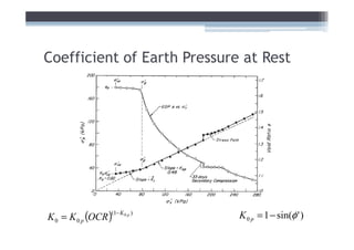
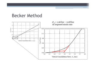
82. Adjust for EOP conditions
[σ ' ]
p ε
&p εp 
&
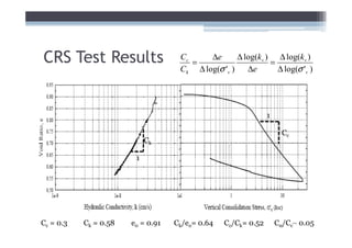
 Cα

C
 C




=  = 0.94
[σ ' ]
p ε
&I
ε 
 &I 
EOP Maximum Past Pressure
σ’p = 1.88 kg/cm2