This document provides copyright information for a book on material science published by NewAge International (P) Ltd. It contains blank pages and a preface written by the authors Bhilwara S.L. Kakani and Amit Kakani in February 2004 thanking the publisher and welcoming suggestions to improve the book. The preface is followed by a table of contents outlining the chapters in the book.


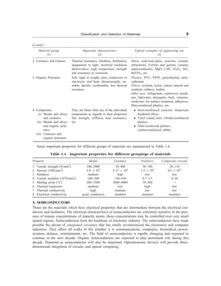
![Classification and Selection of Materials 17
impact and ecological factors, it is becoming more important to consider ‘cradle to grave’ life cycle of
materials relative to overall manufacturing process.
Example 1 What will be the selection criteria for 15 A electrical plugs? [AMIE, Diploma]
Solution The selection criteria for 15 A electrical plugs are
(i) The said electrical plugs are designed for the required amperage.
(ii) The plugs are electrically safe to handle.
(iii) The electrical plugs are cheap to produce.
(iv) The plugs can be produced on mass scale.
(v) While in use, the said plugs should not cause injury.
(vi) The plugs should be rigid enough so that they do not break easily while in use, i.e., handling.
(vii) The size of the pins should be such that these can be easily inserted and removed from the terminal.
Example 2 What will be the selection criteria for a flexible PVC hose pipe? [AMIE, Diploma]
Solution The selection criteria for a flexible PVC hose pipe will be
(i) It should be light in weight.
(ii) It should be flexible and not rigid.
(iii) It should not wear out easily.
(iv) Its surface should be smooth and does not affects the hands while handling.
(v) It should not crack when rolled after use.
(vi) It can be produced on mass scale.
(vii) It should be cheap in comparison to the other products.
SUGGESTED READINGS
1. A. Street and W. Alexander, ‘Metals in the Service of Man’, Penguin Books (1976).
2. Materials, ‘A Scientific American Book’, W. H. Freeman and Co., San Francisco (1968).
3. D. Fishlock, ‘The New Materials’, John Murray, London (1967).
4. J. P. Schaffer, et al., ‘The Science and Design of Engineering Materials’, 2nd Ed., McGraw-Hill
(2000).
5. J. F. Shackelford, ‘Introduction to Materials Science for Engineers’, 5th Ed., Prentice Hall (2000).
6. R. E. Hummel, ‘Understanding Material Science’, Springer-Verlag, New York (1998).
REVIEW QUESTIONS
1. Mention the main properties of metals, polymers and ceramics.
2. Write general properties and characteristics of metals, polymers, ceramics, semiconductors and com-
posite materials. Give few examples belonging to each group.
3. Justify the statement that ‘selection of material is a compromise of many factors’?
4. How metals are classified according to their use?
5. How materials are classified according to their chemical composition?
6. What should be the criteria of selection of material for the construction for chemical process indus-
tries?
7. Explain in brief, why metals in general are ductile, whereas ceramics are brittle?
8. Why it is essential for a materials engineer to have the systematic classification of materials?
9. Write the properties required for a material to withstand high temperatures.
10. Explain the following terms as they relate to metals: alloys, sintered metal, coated metal, clad metal,
and non-ferrous metals. Give atleast two examples of each.
11. Write the important features of inorganic materials.](https://image.slidesharecdn.com/s-230301071329-4f25d7e9/85/S-L-_Kakani-_Material_Science_-New_Age_Pub-_2006-BookSee-org-pdf-34-320.jpg)
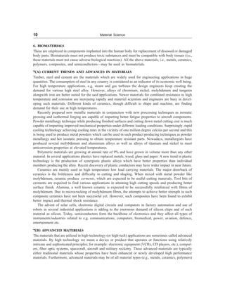
![18 Material Science
12. What do you understand by pozzolanic material?
13. Compare organic and inorganic materials in terms of their structures, properties and characteristics.
14. Write short notes on
(i) Biological materials (ii) Pozzolanic Material
(iii) Effects of tanning on animal hides (iv) Metals
(v) Rocks (vi) Composite Materials
PROBLEMS
1. Explain with specific reason the property you will consider while selecting the material for the
following:
(a) Tyres for an aircraft wheels
(b) A screw driver
(c) Lining for oil fired furnace having temperature ~1200°C.
(d) A 100 mm diameter domestic water pipeline above the ground.
2. Explain, what are the service requirements for the following?
(a) A vacuum cleaner (b) An air conditioner
(c) Electric iron (d) A conveyor belt for handling crushed coal
(e) A car
SHORT QUESTION-ANSWERS
Fill in the blanks
1. Materials Science and engineering draw heavily from engineering sciences such as ,
, and . [metallurgy, ceramics and Polymer Science]
2. What are the three broad groups in which engineering materials can be classified according to their
nature? [Metals and alloys, ceramics and glasses and organic polymers]
3. How the materials can be classified according to major areas in which they are used?
[structures, machines, devices]
4. What are devices?
[These are the most recent addition to engineering materials and refer to such innovations as a
photoelectric cell, transistor, laser, computer, ceramic magnets, piezoelectric pressure gauges, etc.]
5. Microstructure generally refers to the structure as observed under the .
[optical microscope]
6. The optical microscope can resolve details upto a limit of about .
[10–7
m = 0.1 mm]
7. The modern microscope which produces images of individual atoms and imperfections in atomic
arrangements is called . [field ion microscope]
8. In an electron microscope, a magnification of times linear is possible. [105
]
9. What are nuclear spectroscopic techniques for studying nuclear structure?
[NMR and Mössbauer spectroscope]
10. What do you understand by electronic structure of a solid?
11. What are the two categories in which polymers can be classified?
12. What are composites?
13. What are the criteria which affect the selection of a material?
14. What is the difference between macro and micro structures?
15. What is a unit cell in a crystal?](https://image.slidesharecdn.com/s-230301071329-4f25d7e9/85/S-L-_Kakani-_Material_Science_-New_Age_Pub-_2006-BookSee-org-pdf-35-320.jpg)

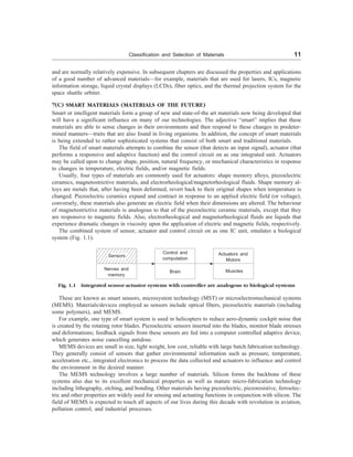
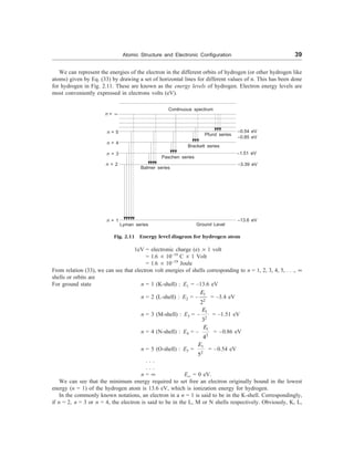
![Atomic Structure and Electronic Configuration 33
Example 2 Calculate the radius and frequency of an electron in the Bohr’s first orbit in hydrogen atom.
Given e0 = 8.854 ´ 10–12
F/m, m = 9.1 ´ 10–31
kg, e = 1.6 ´ 10–19
C, h = 6.625 ´ 10–34
J-s
Solution rn =
2 2
0
2
n h
mZe
e
p
For the first Bohr orbit of hydrogen atom, n = 1 and Z = 1. Thus
r1 =
2 12 34 2
0
2 31 19 2
8.854 10 (6.625 10 )
22
me 9.1 10 (1.6 10 )
7
h
e
p
- -
- -
´ ´ ´
=
´ ´ ´ ´
= 5.3 ´ 10–11
m = 0.53 Å
and orbital frequency
n =
2 4
2 3 3
0
4
mZ e
n h
e
=
31 19 4
12 2 3 34 3
9.1 10 1 (1.6 10 )
4 (8.854 10 ) (1) (6.625 10 )
- -
- -
´ ´ ´ ´
´ ´ ´ ´ ´
= 6.54 ´ 1015
Hz.
Example 3 The radius of first orbit of electron in a hydrogen atom is 0.529 Å. Show that the radius of
the second Bohr orbit in a singly ionized helium atom is 1.058 Å. [AMIE]
Solution For hydrogen: Z = 1, n = 1 and r1 = 0.529 Å
For helium: Z = 2, n = 2 and r2 = ?
The radius of nth Bohr orbit of an atom,
rn =
2 2 2
0
2
mZe
n h n
k
Z
e
p
= (i)
Where k =
2
0
2
h
me
e
p
is a constant
For the first Bohr orbit of electron in hydrogen atom, we have
(r1)H = 0.529 Å = k
2
(1)
1
k = 0.529 Å
For helium (Z = 2), the radius of second Bohr orbit (n = 2), we have
(r2)He = k
2
n
Z
= 0.529 ´
2
2
2
= 1.058 Å
Example 4 Show that the energy released by an electron jumping from orbit 3 to orbit 1 and the energy
emitted by an electron jumping from orbit 2 to orbit 1 are in the ratio 32 : 27. [AMIE]
Solution The energy of an electron in the nth Bohr orbit of an atom is given by
En = –
2
2
13.6Z
n
eV](https://image.slidesharecdn.com/s-230301071329-4f25d7e9/85/S-L-_Kakani-_Material_Science_-New_Age_Pub-_2006-BookSee-org-pdf-50-320.jpg)
![34 Material Science
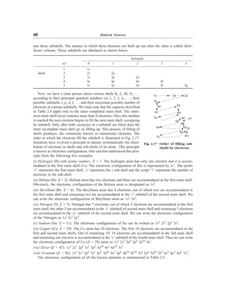
Now, for the first orbit (n = 1),
E1 = –13.6
2
2
(1)
Z
eV
For the second orbit (n = 2),
E2 = –13.6
2
2
( 2)
Z
eV
Similarly for the third orbit (n = 3),
E3 = – 13.6
2
2
(3)
Z eV
Energy emitted by an electron jumping from orbit 3 to orbit 1,
E3 – E1 = –13.6
2
2
2 2
13.6
(3) (2)
Z
Z æ ö
- -
ç ÷
è ø
= –13.6 Z2 1 1
9 1
æ ö
-
è ø
= –13.6 Z2 8
9
æ ö
-
è ø
Similarly, energy emitted by an electron jumping from orbit 2 to orbit 1,
E2 – E1 = –
2
2
2 2
13.6
13.6
(2) (1)
Z
Z æ ö
- -
ç ÷
è ø
= –13.6 Z2 1 1
4 1
æ ö
-
è ø
= –13.6
3
4
æ ö
-
è ø
3 1
2 1
E E
E E
-
-
=
8/9
3/4
= 32 : 27
Example 5 How many revolutions does an electron in the first Bohr orbit of hydrogen make per second.
[B.E.]
Solution The number of revolutions per second = n/2pr
Now, substituting for r and v, one obtains,
Number of revolutions per second
=
2 2 2 2
2 2 2 3 3
0 0 0
mZe
2 2 4
Ze mZ e
nh n h n h
p
e pe e
´ =
Using m = 9.1 ´ 10–31
kg, Z = 1, e = 1.6 ´ 10–19
C,
e0 = 8.85 ´ 10–12
F/m, n = 1, and h = 6.63 ´ 10–34
,
We obtain
Number of rev./sec =
31 19 4
12 2 34 2
9.1 10 (1.6 10 )
4 (8.25 10 ) (6.63 10 )
- -
- -
´ ´ ´
´ ´ ´ ´
= 7.23 ´ 1017](https://image.slidesharecdn.com/s-230301071329-4f25d7e9/85/S-L-_Kakani-_Material_Science_-New_Age_Pub-_2006-BookSee-org-pdf-51-320.jpg)
![Atomic Structure and Electronic Configuration 35
Example 6 Determine the orbital frequency of an electron in the first Bohr’s orbit in a hydrogen atom.
[AMIE]
Solution Given n = 1, Z = 1 for hydrogen atom
The orbital frequency of the electron
nn =
2 4
2 3 3
0
4
mZ e
h n
e
Substituting the values of various constants and simplifying, we obtain
nn = 6.56 ´ 1015
2
3
Z
n
Now, for first Bohr orbit of hydrogen atom
n1 = 6.56 ´ 1015
2
3
(1)
(1)
= 6.56 ´ 1015
Hz.
Example 7 Calculate the values of kinetic energy, potential energy and total energy of an electron in a
hydrogen atom in its ground state. Given e0 = 8.854 ´ 10–12
F/m,
h = 6.625 ´ 10–34
J-s, m = 9.11 ´ 10–31
kg and
e = 1.6 ´ 10–19
c.
Solution For an electron in the ground state orbit of the hydrogen; n = 1 Z = 1
Using relations derived earlier and values of physical constants given, we obtain,
Total energy E = –
31 76
24 60
9.11 10 6.554 10
8 78.39 10 43.89 10
- -
- -
´ ´ ´
´ ´ ´ ´
= –2 ´ 10–18
J = –13.6 eV
K.E. = 13.6 eV
P.E. = –27.2 eV
Example 8 Calculate the velocity of an electron in hydrogen atom in Bohr’s first orbit. Given
h = 6.626 ´ 10–34
J-s, e0 = 8.825 ´ 10–12
F/m and
e = 1.6 ´ 10–19
c.
Solution For hydrogen n = 1, Z = 1
We have nn =
2
0
2
Ze
nh
e
n1 =
19 2
2
12 34
0
(1.6 10 )
e
2 h 2 8.825 10 1.626 10
-
- -
´
=
e ´ ´ ´ ´
m/s
= 2.189 ´ 106
m/s.
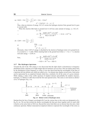
Example 9 Electrons of energies 10.2 eV and 12.09 eV can cause radiation to be emitted from hydrogen
atoms. Calculate in each case: (a) the principal quantum number of the orbit to which electron in the
hydrogen atom is raised and (b) the wavelengths of radiation emitted if the electron drops back to the
ground level. [AMIE]
Solution The electron is excited from n = 1 (ground state) to the excited state n = ? (higher energy level).
During this process of excitation, electron acquires energy of 10.2 eV or 12.09 eV.
We have 2 1
n n
E E
- =
4
2 2 2 2
0 1 2
1 1
8
me
h n n
e
æ ö
-
ç ÷
è ø](https://image.slidesharecdn.com/s-230301071329-4f25d7e9/85/S-L-_Kakani-_Material_Science_-New_Age_Pub-_2006-BookSee-org-pdf-52-320.jpg)
![54 Material Science
3 1 –1 –
1
2
3 0 0
1
2
3 0 0 –
1
2
Example 12 Write the electronic configuration of Sn (Z = 50).
Solution Sn (Z = 50): 1s2
2s2
2p6
3s2
3p6
3d10
4s2
4p6
4d10
5s2
5p2
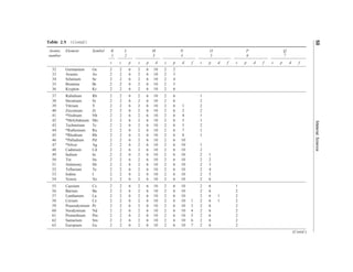
Example 13 Which elements have the following levels filled in the ground state?
(a) K and L shells, the 3s subshell and one half of 3p subshell.
(b) K, L and M shells, the 4s, 4p, 4d and 5s subshells. [BE]
Solution
(a) From Table 2.1, we can have the following table
Shell Principal Quantum No. Subshell No. of electrons
K 1 s 2
L 2 s 2
p 6 Total 15
M 3 s 2
p 3
For filling of subshell we must follow the rule cited earlier. In this case, however, the subshells 1s,
2s, 2p, 3s and 3p fill in sequence.
(b) The subshells will fill in the following order 1s, 2s, 2p, 3s, 3p, 4s, 4d, 5s, 4d
We can prepare the table as follows:
Shell Principal Quantum No. Subshell No. of electrons
K 1 s 2
L 2 s 2
p 6
M 3 s 2
p 6 Total 48
d 10
N 4 s 2
p 6
d 10
O 5 s 2
16. WAVE MECHANICAL PICTURE OF THE ATOM
In 1924 de Broglie suggested that particles in motion should exhibit properties characteristic of waves. He
further suggested that certain basic formulae should apply both to waves and particles. The wavelength of
such particles, e.g., electron, proton, neutron, etc. is given by the relation
l =
h
mv
(36)
where h is Planck’s constant, m is mass of the particle and v is the velocity of the particle. de Broglie called
these waves as matter waves. Relation (36) provides the mathematical relationship between the momentum
(p = mv) of a particle which is a dynamical variable characteristic of a corpuscle and the wavelength which
is characteristic of the associated wave.
ü
ï
ï
ý
ï
ï
þ
ü
ï
ï
ï
ï
ï
ý
ï
ï
ï
ï
ï
þ](https://image.slidesharecdn.com/s-230301071329-4f25d7e9/85/S-L-_Kakani-_Material_Science_-New_Age_Pub-_2006-BookSee-org-pdf-71-320.jpg)
![58 Material Science
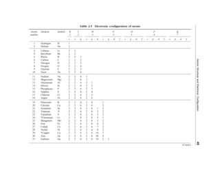
(iv) f-block: The elements, whose valence electrons lie in the f-sub-shell are known as f-block elements.
These are shown at the bottom of the periodic table.
The modern periodic table is also divided into seven horizontal rows or periods. These are:
(i) First Period: This contains two elements having atomic numbers 1 and 2. The element with Z = 1 lies
in group IA of s-block and that with Z = 2 in group zero of p-block. This period is also known as short
period.
(ii) Second Period: This contains eight elements with atomic number 3 to 10. The elements with Z = 3,
4 lie in group IA and IIA of s-block and those with atomic number 5 to 10 in groups IIIA to zero in
p-block. This is also known as short period.
(iii) Third Period: This contains eight elements with Z = 11 to 18. The elements with Z = 11, 12 lie in
groups IA and IIA of s-block and those with Z = 13 to 18 in groups IIIA to zero in p-block. It is also called
as a short period.
(iv) Fourth Period: This contains 18 elements with Z = 19 to 36. The elements with Z = 19 and 20 lie in
s-block, elements with Z = 21 to 30 in d-block and Z = 31 to 36 in p-block. This is known as a long period.
(v) Fifth Period: This contains 18 elements with Z = 37 to 54. The elements with Z = 37 and 38 lie in
s-block, with Z = 39 to 48 in d-block and Z = 49 to 54 in p-block. This is also known as a long-period.
(vi) Sixth Period: This contains 32 elements with Z = 55 to 86. The elements with Z = 55, 56 lie in the
s-block, Z = 57 and 72 to 80 in d-block, Z = 58 to 71 in f-block and Z = 81 to 86 in p-block. This is known
as very long period.
(vii) Seventh Period: This contains the remaining elements with Z = 87 to 105. The elements with Z = 87,
88 lie in s-block, Z = 89, 104 and 105 lie in d-block and Z = 90 to 103 in f-block. This period of elements
is still incomplete.
The elements with Z = 58 to 71 in f-block are called lanthanides, all the elements in d-block are called
transition elements and those with Z = 90 to 103 are actinides. The elements belonging to lanthanides and
actinides have similar properties and hence they have been placed at the bottom of the periodic table. The
actinides do not occur in nature and are prepared artificially.
Elements on the left hand side of the diagonal dividing band are known as ‘metals’ whereas those on
the right are called ‘non-metals’ and those within the band are called ‘semi-metals’ or ‘metalloides’.
The periodic table is very useful in solving the problem of scarcity, e.g. during World War II, scientists
and engineers solved the problem of scarcity ‘tungsten’ by engineering application of the Periodic Table.
18% tungsten tool steel was substituted by 8% molybdenum and 2% tungsten, which is even used today.
This was possible, because molybdenum is placed directly above the tungsten in the periodic table of
elements.
Example 13 Assuming that the weight of an electron is negligible compared to the weight of proton and
neutron, calculate the weight of copper atom. Assuming that weight of one proton is equal to that of one
neutron, find the weight of one proton. [AMIE]
Given, Atomic weight of copper = 63.54,
Avogadro’s numbers (N) = 6.023 ´ 1023
atoms/gm-mole.
Solution N= 6.023 ´ 1023
atoms/gm-mole
Weight of 1 atom =
23
63.54
6.023 10
´
= 1.054 ´ 10–22
gm
Now, Atomic Weight = No. of protons + No. of neutrons
We have (no. of protons + no. of neutrons)/atom = 63
Weight of 1 proton =
22
1.054 10
63
-
´
= 1.673 ´ 10–23
gm](https://image.slidesharecdn.com/s-230301071329-4f25d7e9/85/S-L-_Kakani-_Material_Science_-New_Age_Pub-_2006-BookSee-org-pdf-75-320.jpg)
![Atomic Structure and Electronic Configuration 59
Example 14 Using conventional s, p, d, f, . . . notations, write the electronic configuration of Fe atom
(Z = 26) and Fe2+
and Fe3+
ions. [BE, AMIE]
Solution We have the capacity of subshells as
s – 2, p – 6, d – 10 and f – 14
Electronic configuration of Fe atom is
1s2
2s2
2p6
3s2
3p6
3d6
4s2
Fe2+
ions means the Fe atom has lost 2 electrons of the outermost orbit which is 4s. Thus the electronic
configuration of Fe2+
is
1s2
2s2
2p6
3s2
3p6
3d6
Fe3+
ions means the Fe atom has lost 3 electrons, i.e. one more than Fe2+
ion. Obviously the loss of one
electron will occur from 3d electrons. We can write the electronic configuration as
1s2
2s2
2p6
3s2
3p6
3d5
Example 15 Atomic weight of Cu and Si are 63.54 and 28.09 respectively. Find the percentage of Si in
Cu5 Si. [AMIE, BE]
Solution The percentage of Si in Cu5 Si is =
28.09
63.54 28.09
+
´ 100 = 8.12%
SUGGESTED READINGS
1. L. Solymar and D. Walsh, ‘Lectures on the Electrical Properties of Materials’, Oxford University
Press, Oxford (1984)
2. H.H. Sisler, Electronic structure, Properties and the Periodic Law, Reinhold Pub. Cooperation, New
York (1963)
3. W.L. Masterton and C.N., Hurley, Chemistry, Principles and Reactions, 2nd Ed. Harcourt, Fort
Worth, TX, (2000)
4. S.L. Kakani, Modern Physics, Viva Books Publishers, New Delhi (In Press)
REVIEW QUESTIONS
1. What is an atom? Describe briefly the important constituents of an atom.
2. Explain the simplified concept of an atom and the significance of the same in relation to properties
of bulk materials. [AMIE, B.E.]
3. State and explain Bohr’s model of an atom. [AMIE]
4. In Bohr’s theory of hydrogen atom the principal quantum number n cannot take the value zero.
Explain.
5. State the basic postulates of Bohr’s atom model.
6. Deduce an expression for the radius of the electron orbit in the hydrogen atom.
7. Deduce an expression for the binding energy of an electron in a hydrogen like atom according to
Bohr’s theory.
8. How does Bohr’s model account for the different spectral series of the hydrogen atom?
9. Obtain an expression for the energy of the electron in the nth orbit in hydrogen atom.
10. According to Bohr’s theory, the potential energy of electron in a hydrogen atom is negative and larger
in magnitude than the kinetic energy. Explain the significance of this. [BE]
11. Give a brief account of Sommerfeld’s modification of Bohr’s theory. What was the need for this
modification.](https://image.slidesharecdn.com/s-230301071329-4f25d7e9/85/S-L-_Kakani-_Material_Science_-New_Age_Pub-_2006-BookSee-org-pdf-76-320.jpg)
![60 Material Science
12. Explain atomic mass and mass number. What is an isotope? [AMIE]
13. What is Pauli’s exclusion principle and how it is applied to atom’s electronic structure? [AMIE]
14. What is modern concept about the structure of an atom? Describe briefly.
15. What do you understand by the electronic configuration? [AMIE]
16. Write electronic configuration of iron. [AMIE]
17. Explain the difference between atomic weight and atomic number and their importance in the periodic
table. [AMIE]
18. Explain how atomic shells and sub-shells are formed. [AMIE]
19. Justify the Mosley’s law on the basis of Bohr’s theory. [AMIE]
20. Explain, how the experiment on a-particle scattering led to the concept of the nuclear model of the
atom. [AMIE, BE]
21. Explain how the modern periodic table is different from Mandeleev’s periodic table. [AMIE]
22. What is the basis on which periodic table is divided into four blocks?
23. Differentiate between periods and groups in a periodic table.
24. What is deuterium. Write its electronic configuration.
25. Why elements with zero valence electrons are called ‘inert gases’? [AMIE]
26. Show that potential energy = –2 kinetic energy for an electron in a circular orbit in Coulomb field.
[AMIE]
27. Define the following
(i) Atomic structure (ii) Atomic number
(iii) Molecule (iv) Nucleus
(v) Proton (vi) Neutron
(vii) Electron [AMIE]
28. State the fundamental postulates of Bohr’s theory and explain hydrogen spectrum. [AMIE]
29. Write short notes on:
(i) Ruther-ford’s nuclear atom model
(ii) The spectrum of hydrogen [AMIE]
(iii) Bohr’s postulates [AMIE]
(iv) Sommerfeld-Wilson atomic model
(v) Pauli’s exclusion principle
(vi) Vector Atom model
(vii) Non-acceptance of Thomson’s model of an atom. [AMIE]
30. Explain the following
(a) Isotopes (b) Isobars
(c) nucleon (d) atomic mass
(e) atomic number (f) alpha particle
(g) meson (h) nucleus.
PROBLEMS
1. Calculate the radius of the first orbit of the electron in the hydrogen atom. Given,
h = 6.626 ´ 10–34
J.s, m = 9.11 ´ 10–31
kg and e = 1.6 ´ 10–19
C. [Ans. 5.315 ´ 10–11
m]
2. Calculate the velocity of the electron in the innermost orbit of the hydrogen atom.
[Ans. 2.2 ´ 103
m/s]
3. The wavelength of the first line of the Balmer series of hydrogen is 656.3 nm. Calculate the Rydberg
constant. [Ans. 1.097 ´ 107
m–1
]
4. The radius of the first orbit in a hydrogen atom is 0.053 nm. Calculate the velocity of the electron
in this orbit. [Ans. 2.186 ´ 106
m/s]](https://image.slidesharecdn.com/s-230301071329-4f25d7e9/85/S-L-_Kakani-_Material_Science_-New_Age_Pub-_2006-BookSee-org-pdf-77-320.jpg)
![Atomic Structure and Electronic Configuration 61
5. The Rydberg constant for hydrogen is 10967700 m–1
. Find the short and long wavelength limits of
the Lyman series. [Ans. 91.16 nm; 121.5 nm]
SHORT QUESTIONS
1. How does the Thomson atom model differ from a random distribution of protons and neutrons in a
spherical region?
2. Write objections to the Thomson model of the atom.
3. The scattering of a-particles at very small angles disagrees with the Rutherford’s formula for such
angles. Explain.
4. Did Bohr postulate the quantization of energy? What did he postulate?
5. Does the Rydberg constant vary with the nucleus? Explain.
6. Can a hydrogen atom absorb a photon whose energy is more than the binding energy?
7. Explain the need for introducing the concept of electron spin.
OBJECTIVE QUESTIONS
1. The charge carriers in the discharge tube at very low pressures are and
(electrons, positive ions)
2. Rydberg’s constant varies with the of a given element. (mass number)
3. Photons do not have a finite (rest mass)
4. The different lines in the Lyman series have their wavelength lying between Å and
Å. (911, 1215)
5. If elements with principal quantum number n 4 were not allowed in nature, then the number of
possible elements would be (60)
[Hint: The maximum number of electrons allowed in an orbit being 2n2
. The required number is
2 ´ (12
+ 22
+ 32
+ 42
) = 60].
6. If the angular momentum of the earth due to its motion around the sun were quantized according to
Bohr’s relation L = nh/2p, then the quantum number corresponding to this quantization would be
(2.5 ´ 1074
)
7. State whether the following statements are True or False:
(a) The mass of an electron is greater than the mass of a proton. (False)
(b) Atomic number of an element is equal to the number of protons present in the nucleus.(True)
(c) The mass number of an element is the sum of the number of protons and neutrons present in the
nucleus of the element. (True)
(d) All atoms having different atomic weights but belonging to the same element are called isobars.
(False)
(e) The nucleus is normally composed of protons and neutrons. (True)
(f) The orbital quantum number (l) is also known as the azimuthal quantum number. (True)
(g) Transition elements have higher melting points and higher densities as compared to light metals.
(True)
(h) The elements which occupy the seventh row of the periodic table but do not occur in nature and
are prepared artificially are called actinides. (True)
8. Fill in the blanks
(a) 1 eV = __________J. (1.6 ´ 10–19
)
(b) Rydberg constant (R) of hydrogen formula
= __________ m–1
(1.097 ´ 107
)
(c) The mass of an electron is __________ kg. (9.1 ´ 10–31
)](https://image.slidesharecdn.com/s-230301071329-4f25d7e9/85/S-L-_Kakani-_Material_Science_-New_Age_Pub-_2006-BookSee-org-pdf-78-320.jpg)
![72 Material Science
Vc = [ ]
a b c
®
® ®
× ´ (1)
where Vc stands for the volume of the cell and a
®
, b
®
and c
®
defined so far as the measure of the unit cell
edges, are commonly known as lattice parameters.
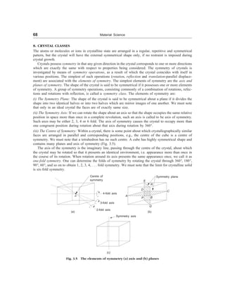
Now, we shall discuss about the seven type of basic systems mentioned in Table 3.1.
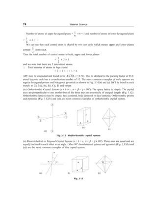
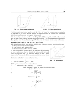
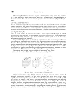
(i) Cubic Crystal System: (a = b = c, a = b = g = 90°): All those crystals which have three equal axes and
are at right angles to each other and in which all the atoms are arranged in a regular cube are said to be
cubic crystals (Fig. 3.8). The most common examples of this system are cube and octahedron as shown in
Fig. 3.8(a) and (c). In a cubic crystal system, we have
a = b = c, a = b = g = 90°
Z
a
a
a
X
(a)
1
1
1
1
1
1
90°
90°
90°
90°
90°
90°
(b) (c)
Fig. 3.8 Cubic Crystal System
Atomic Packing Factor (APF): This is defined as the ratio of total volume of atoms in a unit cell to the
total volume of the unit cell. This is also called relative density of packing (RDP).
Thus
APF =
No. of atoms volume of one atom
volume of unit cell
v
V
´
= (2)
In a simple cubic cell, no. of atoms in all corners
=
1
8
´ 8 = 1
Radius of an atom = r and volume of cubic cell = a3
= (2r)3
(Q a = 2r)
APF =
3
3
4
1
3
6
(2 )
r
r
p
p
´
= (= 0.52) = 52%
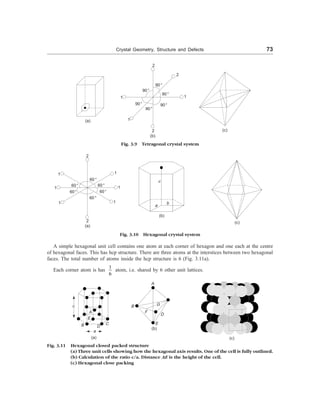
(ii) Tetragonal Crystal System: (a = b ¹ c, a = b = g = 90°). This includes all those crystals, which have
three axes at right angles to each other and two of these axes (say horizontal) are equal, while the third (say
vertical) is different (i.e., either longer or shorter than the other two). Figure 3.9(b) shows a tetragonal
crystal system. The most common examples of this system of crystals are regular tetragonal and pyramids
(Fig. 3.9(a) and (c))
(iii) Hexagonal Crystal System: (a = b ¹ c, a = b = g = 90°, g = 120°): All those crystals which have four
axes falls under this system. Three of these axes (say horizontal) are equal and meet each other at an angle
of 60° and the fourth axis (say vertical) is different, i.e. either longer or shorter than the other three axes.
(Fig. 3.10(a)).](https://image.slidesharecdn.com/s-230301071329-4f25d7e9/85/S-L-_Kakani-_Material_Science_-New_Age_Pub-_2006-BookSee-org-pdf-89-320.jpg)
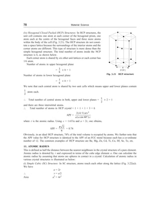
![80 Material Science
=
A
M
N
´ n
(n ® number of atoms per unit cell and NA ® Avogadro’s number, M ® the atomic weight, and a ® side
of a cubic unit cell).
=
3
A
nM
a N
(i) Linear density: This is defined as the number of atoms per unit length along a specific crystal direction.
(ii) Planar density: This is defined as the number of atoms per unit area on a crystal plane. This affect
significantly the rate of plastic deformation.
13. DIRECTIONS, LATTICE PLANES AND MILLER INDICES
In a crystal there exists directions and lattice planes which contain a large concentration of atoms. Various
properties of crystals, particularly mechanical are connected with the structure of the crystal though the help
of crystal directions. A complete description of the crystal structure can be obtained from the study of
atomic positions in a unit cell. For crystal analysis it is necessary to locate directions and lattice planes.
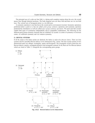
(i) Crystal Directions: To specify the direction of a straight line joining lattice points in a crystal lattice,
we choose any lattice point on the line as the origin and express the vector joining this to any other lattice
point on the line as follows:
r
®
= 1 2 3
n a n b n c
®
® ®
¢ ¢ ¢
+ + (3)
R
Q
z
O
P
x
b
a
c
y
[101]
[100]
[111]
Fig. 3.22(d) Crystal directions in a
orthorhombic lattice
identical to the direction [111]. As stated earlier, in such cases lowest combination of integers, i.e. [111]
is used to specify the direction.
We must note that there are other directions, not parallel to the one under consideration which are
equivalent to the given direction by virtue of rotation symmetry. Thus, the equivalent directions of [100]
are [010], [001], [100], [010] and [001], where the bars denote the negative values. By all possible
positive and negative combinations of indices, we obtain a family of directions. In the present example, all
these six equivalent directions are grouped together in the symbol 100, where the bracket represents
the whole family.
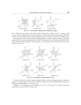
(ii) Crystallographic Planes: The crystal lattice may be regarded as made-up of an aggregate of a set of
parallel equidistant planes, passing through the lattice points, which are known as lattice planes, or atomic
planes. For a given lattice, one can choose the lattice planes in different ways as shown in Fig. 3.23. These
crystal planes and crystal directions play an important role in hardening reaction, plastic deformation and
other properties as well as behaviour of metal. Crystal planes in cubic structures are shown in Fig. 3.24.
The direction of the line is represented by the set of integers
1 2
,
n n
¢ ¢ and 3
n¢. If these integer numbers have common factors, they
are removed and the direction is denoted by [n1, n2, n3]. More-
over, this line also denotes all lines parallel to this line. In Fig.
3.22(d), three different directions are shown in the orthorhombic
lattice. The direction [111] is the line passing through the origin
O and point P. It may be noted that the point P is at a unit cell
distance from each axis. The direction [100] is the line passing
through origin O and point Q. Obviously, the point Q is at a
distance 1, 0, 0 from x, y and z axes respectively. The direction
[101] is the line passing through the origin O and the point R.
Again, the point R is at a unit cell distance of 1, 0, 1 from x, y
and z axes respectively.
In specifying crystal directions, we have taken crystal axes as
base directions. We must note that directions [333] or [222] are](https://image.slidesharecdn.com/s-230301071329-4f25d7e9/85/S-L-_Kakani-_Material_Science_-New_Age_Pub-_2006-BookSee-org-pdf-97-320.jpg)
![82 Material Science
1 1 1
: :
2 3 1
= 3 : 2 : 6
Obviously, Miller indices are defined as the reciprocals of the intercepts made
by the plane on the crystallographic axes when reduced to smallest numbers.
We must remember that all planes have same indices. If negative sections are
cut off by the plane, this is indicated by a bar above the corresponding index,
e.g. 1 (Fig. 3.26).
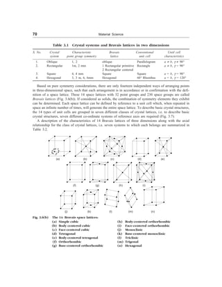
Figure 3.27 shows the planes in a cubic structure. We can easily see that
the Miller indices of the sides of a unit cell of a cubic lattice are (100), (100),
(010), (010), (001) and (001). These planes are planes of the same form, i.e.
equivalent planes and are collectively represented by {100} and are called
families of planes.
(010)
z
x (111)
(010)
y
Fig. 3.26 Miller indices
[001]
z
[010]
y
[100]
x
(a)
z
y
x
[ 1 01]
(b)
z
y
x
(020)
(c)
z
y
x
(110)
(d)
z
y
x
[111]
(e)
z
y
x
(f)
Fig. 3.27 Lattice planes in a cubic system. Negative intercepts are indicated on negative coordinates
The lattice or crystallographic direction can be defined as a line joining any two points of the lattice.
Using a similar notation, we can describe the direction of a line in a lattice with respect to the unit vectors.
We know that Miller indices of a direction are simply the vector components of the direction resolved along
each of the co-ordinate axis, expressed as multiples of the unit cell parameters and reduced to their simplest
form. They are denoted by [hkl] (to distinguish it from the (hkl) plane).
Just like the principal planes of importance, the directions with which one is mainly concerned are [110],
[100] and [111]. We note that these are, respectively, a cube face diagonal, a cube edge and a body
diagonal. We can label the families of directions by special brackets as are families of planes. Obviously,
100 denotes the family of directions which includes [100], [010], [001], [100], [010] and [001]. Figure
3.27 (g) and (h) shows the Miller indices for directions: (i) cubic lattice system and (ii) Hexagonal lattice
system.
[ 1 11]](https://image.slidesharecdn.com/s-230301071329-4f25d7e9/85/S-L-_Kakani-_Material_Science_-New_Age_Pub-_2006-BookSee-org-pdf-99-320.jpg)
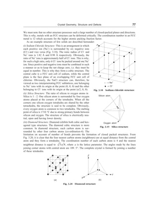
![Crystal Geometry, Structure and Defects 83
c
[ 1 01]
a
[110]
[101]
[111]
b
(g) Cubic lattice system
d
a
b
(h) Hexagonal system
Fig. 3.27 Miller indices for directions
(iv) Important Features of Miller Indices of Crystal Planes: A few important features of Miller indices of
crystal planes are:
(a) All the parallel equidistant planes have the same Miller indices. Obviously, Miller indices define a
set of parallel planes.
(b) A plane parallel to one of the coordinate axis has an intercept of infinity (¥) and therefore the Miller
index is zero.
(c) If the Miller indices of the two planes have the same ratio (i.e., say 844 and 422 or 211), then the
planes are said to be parallel to each other. In other words, all equally spaced parallel planes with
a particular orientation have the same index number [hkl].
(d) Only the ratio of indices is important.
(e) Miller indices of planes are denoted by (hkl), i.e., the plane cuts the axes into h, k and l equal
segments. The directions in space are represented by square bracket [xyz].
(f) The common inside brackets are used separately and not combined. Obviously, (111) is read as one-
one-one and not ‘one hundred eleven’.
(g) Miller indices may also be negative and negative indices are represented by putting a bar over the
digit, e.g. (010).
14. INTERPLANAR SPACINGS
These are the distances between planes and are represented by a number of parts of the body diagonal of
a unit cell. In terms of Miller indices, the distance between planes can be calculated. Let us consider a plane
c
120°
with Miller indices (hkl). This has intercepts a/h, b/k and c/l on the
three axes x, y and z respectively as shown in Fig. 3.28(a). If d is
the length of the normal from the origin, O to the plane and a¢,
b¢ and g ¢ are angles which the normal makes with the coordinates
axes, considered orthogonal, then we have
d =
a
h
cos a¢ =
b
k
cos b¢ =
c
l
cos g ¢
Since cos2
a¢ + cos2
b¢ + cos2
g¢ = 1, we have Fig 3.28(a) Calculation of
interplanar spacings
z
x y
A B
C
O
g ¢
N
b¢
a ¢](https://image.slidesharecdn.com/s-230301071329-4f25d7e9/85/S-L-_Kakani-_Material_Science_-New_Age_Pub-_2006-BookSee-org-pdf-100-320.jpg)
![84 Material Science
dhkl =
2 2 2
2 2 2
1
h k l
a b c
+ +
(4)
dhkl gives the distance between two successive (hkl) places.
For a cubic system: a = b = c
dhkl =
2 2 2
a
h k l
+ +
(5)
For a cubic system lattice, the direction [hkl] is perpendicular to the plane (hkl).
There are three d111 interplanar spacings per long diagonal (body diagonal) of a unit cell in an FCC
structure. We must note that relation (4) is valid for orthogonal lattices only. For non-orthogonal lattices,
such an expression may not be obtained easily.
14(a). ANGLE BETWEEN TWO PLANES OR DIRECTIONS
Let us consider a cube having two planes ABCD and EFCD inclined at an angle q with each other
(Fig. 3.28(b)). Let h1, k1, l1 are Miller indices of plane ABCD and h2, k2 and l2 are Miller indices of plane
EFCD.
The angle between these two planes is given by the relation
cos q =
1 2 1 2 1 2
2 2 2 2 2 2
1 1 1 2 2 2
h h k k l l
h k l h k l
+ +
+ + ´ + +
(6)
Similarly, the angle f between the two directions having
Miller indices (h1, k1, l1) and (h2, k2, l2) respectively is given
by the relation
cos f =
1 2 1 2 1 2
2 2 2 2 2 2
1 1 1 2 2 2
h h k k l l
h k l h k l
+ +
+ + + +
(7)
15. REPRESENTATION OF CRYSTAL PLANES IN A CUBIC UNIT CELL
(100), (010) and (001) represent the Miller indices of the cubic planes ABCD, BFGC and AEFB
respectively (Fig. 3.29).
z
E
A
H
B
D C
x
G
F
y
(a) Plane (100)
z
E
F
A B
H
C
D
G
y
x
(b) Pane (010)
z
E
A B
H
F
y
x D C
(c) Plane (001)
Fig. 3.29 Crystal planes of a cubic unit cell
Obviously, the above mentioned three planes represent the three faces of the cubic unit cell. We can
represent the other three faces of the cube by shifting the origin of the coordinate system to another corner
of the unit cell, e.g. the plane EFGH may be represented by shifting the origin from point H to point D
G
A
B
D E
C F
q
Fig. 3.28(b) Angle between two planes](https://image.slidesharecdn.com/s-230301071329-4f25d7e9/85/S-L-_Kakani-_Material_Science_-New_Age_Pub-_2006-BookSee-org-pdf-101-320.jpg)
![88 Material Science
or a = 4
3
r
In FCC structure, the atoms touch along the face diagonals,
2 a = 4r
or a = 2 2 r.
Example 2 An atomic plane in a crystal lattice makes intercept of 3a, 4b and 6c with the crystallographic
axes where a, b and c are the dimensions of the unit cell. Show that the Miller indices of the atomic plane
are (432).
Solution In terms of the lattice constants, the intercepts are 3, 4 and 6. Their reciprocals are 1/3, 1/4,
1/6. On reducing to a common denominator, they become 4/12, 3/12 and 2/12. Obviously, the Miller indices
of the plane are (432).
Example 3 In a single cubic crystal find the ratio of the intercepts on the three axes by (123) plane.
Solution The reciprocals of Miller indices are 1/1, 1/2 and 1/3. On reducing to a common denominator
they become 6, 3 and 2. Intercepts on the three axes are 6a, 3b and 2c, where a, b and c are the lattice
constants along the three axes.
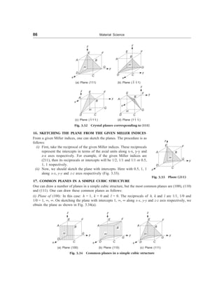
Example 4 Draw (101) and (111) planes in a unit cubic cell. Find the Miller indices of the directions
which are common to both the planes.
Solution Intercepts of the plane (101) with the three axes are 1/1,
1/0 and 1/1 i.e. 1, ¥ and 1. Similarly, the intercepts of the (111) with
the three axes are 1/1, 1/1 and 1/1, i.e. 1, 1 and 1.
Now, taking the point O as origin and lines OA, OB and OC as the
axes a, b and c respectively, the plane with the intercepts 1, ¥ and 1
is the plane ADGC and that with intercepts 1, 1 and 1 is plane ABC
(Fig. 3.36). From figure, it is obvious that the line common to both
the planes is the line AC. This line corresponds to two directions, i.e.,
AC and CA.
Projections of the direction AC on the axes are –1, 0 and 1. Pro-
jections of direction CA on the axes are 1, 0 and –1.
Thus the required indices are [101] and [101].
Example 5 Draw the following planes and directions in the case of a FCC structure: (112), (001) and
(101).
Solution (i) Plane and direction (112): In this, we have h = 1, k = 1 and l = 2. The reciprocals of h, k
and l are 1/1, 1/1, 1/2, i.e. 1, 1, 0.5.
Now, we can sketch the plane with intercepts 1, 1, 0.5 along x-x, y-y and z-z axes respectively
(Fig. 3.37(a).
C G
F
A
B
D
(101)
(111)
O
a
c
Fig. 3.36 Planes (101) and (111)
in a simplecubiclattice
E
z
x
y
z
y
x
(a) Plane (112) (b) Plane (001)
z
y
x
(c) Plane (101)
Fig. 3.37
b](https://image.slidesharecdn.com/s-230301071329-4f25d7e9/85/S-L-_Kakani-_Material_Science_-New_Age_Pub-_2006-BookSee-org-pdf-105-320.jpg)
![90 Material Science
z
x
y
(a) Plane (020)
z
x
y
(b) Plane (120)
z
x
y
(c) Plane (220)
Fig. 3.40
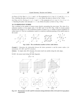
Example 9 Draw the planes and directions of FCC structures (321), (102), (201) and (111).
[B.E. 2001]
Solution (i) Plane and Direction of (321): Here h = 3, k = 2, and l = 1. The reciprocals are 1/3, 1/2,
1/1, i.e. 0.3, 0.5, 1. The sketch of the plane with intercepts 0.3, 0.5 and 1 is as shown in Fig. 3.41(a). A
line drawn normal to this sketched plane and passing through the origin gives the required direction.
z
(321)
x
1/3
y
1/2
[3, 2, 1]
(a)
z
[102]
x
y
(102)
(b)
z
[201]
x
y
(201)
z
[111]
x
y
(111)
(c) (d)
Fig. 3.41
(ii) Plane and Direction of (102): Here h = 1, k = 0, and l = 2. The reciprocals of these are: 1/1, 1/0 and
1/2, i.e. 1, ¥, 0.5. The sketch of the plane with these intercepts is as shown in Fig. 3.41(b). A line drawn
normal to this sketched plane and passing through the origin gives the required direction.
(iii) Plane and Direction of (011): Here h = 0, k = 1, and l = 1. The reciprocals of h and k, l are: 1/0,
1/1, 1/1, i.e. ¥, 1.1. The sketch of the plane with these intercepts is shown in Fig. 3.41(c). A line drawn
normal to this sketched plane and passing through the origin gives the required direction.
(iv) Plane and Direction of (001): Here h = 0, k = 0, and l = 1. The reciprocals of h, k and l are: 1/0,
1/0, 1/1, i.e. ¥, ¥, 1. The sketch of the plane with these intercepts is shown in Fig. 3.41(d). A line drawn
normal to this sketched plane and passing through the origin gives the required direction.](https://image.slidesharecdn.com/s-230301071329-4f25d7e9/85/S-L-_Kakani-_Material_Science_-New_Age_Pub-_2006-BookSee-org-pdf-107-320.jpg)
![Crystal Geometry, Structure and Defects 91
Example 10 In a cubic unit cell, find the angle between normals to the planes (111) and (121).
Solution Since the given crystal is cubic, the normals to the planes (111) and (121) are the directions
[111] and [121] respectively. If q be the angle between the normals, then
cos q =
1 2 1 2 1 2
1/2 1/ 2
2 2 2 2 2 2
1 1 1 2 2 2
h h k k l l
h k l h k l
+ +
+ + + +
=
2 2 2 1/ 2 2 2 2 1/2
1 1 1 2 1 1
(1 1 1 ) (1 2 1 )
´ + ´ + ´
+ + + +
= 0.9428
q = 19.47° or 19° 28¢
Example11 Determine the packing efficiency and density of sodium chloride from the following data:
(i) radius of the sodium ion = 0.98 Å, (ii) radius of chlorine ion = 1.81 Å (iii) atomic mass of sodium =
22.99 amu and atomic mass of chlorine = 35.45 amu.
Solution The unit cell structure of NaCl is shown in Fig. 3.18. We can see that the Na+
and Cl–
ions touch
along the cube edges.
Lattice parameter, a = 2 (radius of Na+
+ radius of Cl–
)
= 2(0.98 + 1.81) = 5.58 Å
Atomic Packing Fraction =
Volume of ions present in the unit cell
Volume of the unit cell
=
+
3 3
Na Cl
3
4
4(4/3) 4
3
r r
a
p p -
æ ö
+
è ø
=
3 3
3
(0.98) (1.81)
16
3 (5.58)
p é ù
+
ê ú
ê ú
ë û
= 0.663 or 66.3%
Density =
Mass of the unit cell
Volume of the unit cell
=
27
10 3
4(22.99 + 35.45) 1.66 10
(5.58 10 )
-
-
´ ´
´
kg/m3
= 2234 kg/m3
or 2.23 gm/cm3
Example 12 Aluminium has FCC structure. Its density is 2700 kg/m3
. Find the unit cell dimensions and
atomic diameter. Given at. weight of Al = 26.98. [Roorkee]
Solution Density =
3
nm
a
NA
= 2700 kg/m3
= 2.7 gm/cm3
=
3 23
4 26.98
6.023 10
a
´
´ ´
a3
=
23
4 26.98
2.7 6.023 10
´
´ ´
= 6.6 ´ 10–23
/cm3
a = 4.048 ´ 10–10
m = 4.048 Å](https://image.slidesharecdn.com/s-230301071329-4f25d7e9/85/S-L-_Kakani-_Material_Science_-New_Age_Pub-_2006-BookSee-org-pdf-108-320.jpg)
![92 Material Science
For FCP structure, r =
4.048Å
2 1.414 2 1.414
a
=
´ ´
= 1.43 Å
Diameter = 2r = 2.86 Å
Example 13 Find the interplanar distance of (200) plane and (111) plane of Nickel crystal. The radius
of Nickel atom is 1.245 Å. [Jodhpur]
Solution Nickel has FCC structure. Given radius of Nickel = r = 1.245 Å
Lattice constant = a =
4 1.245
4
2 2
r ´
= = 3.52 Å
d200 =
2 2 2
3.52
2 0 0 )
+ +
= 1.76 Å
d111 =
2 2 2
3.52
1 1 1
+ +
= 2.03 Å
Example 14 The lattice constant of a unit cell of KCl crys-
tal is 3.03 Å. Find the number of atoms/ mm2
of planes (100),
(110) and (111). KCl has simple cubic structure.
[B.E]
Solution a = 3.03 Å = 3.03 ´ 10–7
mm.
(100) plane The number of atoms in the (100) plane of a
C
(111) (110)
E1
F G
O B
A D
[ 110]
Fig. 3.42 Plane in a unit cell of FCC
Nickel
simple cubic structure
=
2 7 2
1 1
(3.03 10 )
a -
=
´
= 10.9 ´ 1012
(110) plane The number of atoms in (110) plane of a simple cubic structure
=
2 7 2
0.707 0.707
(3.03 10 )
a -
=
´
= 7.7 ´ 1012
(111) plane The number of atoms in (111) plane of a simple cubic structure
=
2 7 2
0.58 0.58
(3.03 10 )
a -
=
´
= 6.3 ´ 1012
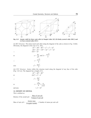
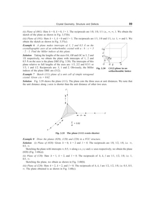
Example 15 Determine the planar density of Ni (FCC
structure) in (100) plane. Given, the radius of Ni atom
= 1.245 Å.
Solution From Fig. 3.43, we have
Number of atoms in (100) plane
= 1 +
1
4
´ 4 = 2
Area of plane = a2
,
= a =
4
2
r
= 3.52 Å Fig. 3.43 Interplanar distances in Ni
crystal
4r
a](https://image.slidesharecdn.com/s-230301071329-4f25d7e9/85/S-L-_Kakani-_Material_Science_-New_Age_Pub-_2006-BookSee-org-pdf-109-320.jpg)
![Crystal Geometry, Structure and Defects 93
Planar density =
7 2
2
(3.52 10 mm )
-
´
= 16.1 ´ 1012
atoms/mm2
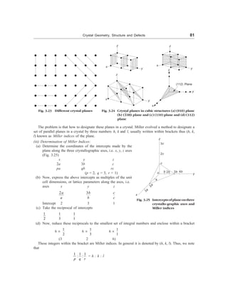
Example 16 Calculate the planar atomic densities of planes (100), (110) and (111) in FCC unit cell and
apply your result for lead (FCC form). [AMIE]
Solution (i) Plane (100): Fig. 3.44(a) shows an FCC unit cell with planes (111) and (111). Figure 3.44(b)
shows the plane (100) with atoms on it. Similarly Figs. 3.44(c) and (d) shows the planes (110) and (111)
with atoms contained in them respectively.
b
(111)
a
c
(a)
(110)
(110)
(b) (c)
2 a
(d) 2 a
Fig. 3.44 Distribution of atoms in planes (100), (110) and (111) in FCC unit cell
Number of atoms contained in (100) plane is 4 ´
1
4
+ 1 = 2
Let a be the edge of the unit cell and r the radius of the atom, then
a = 2 2 r
Planar density of plane (100)
=
2 2
0.25
2
4 2r r
=
´
The radius of lead atom is 1.75 Å. The planar density of (100) plane of lead
=
7 2
0.25
(1.75 10 )
-
´
= 8.2 ´ 1012
atoms/mm2
= 8.2 ´ 1018
atoms/m2
(ii) Plane (110): From Fig. 3.44(c), we have the number of atoms contained in plane (110)
= 4 ´
1
4
+ 2 ´
1
2
= 2](https://image.slidesharecdn.com/s-230301071329-4f25d7e9/85/S-L-_Kakani-_Material_Science_-New_Age_Pub-_2006-BookSee-org-pdf-110-320.jpg)
![94 Material Science
The top edge of the plane (110) is 4r, whereas the vertical edge = a = 2 2 r. Thus the planar density
of (110)
=
2
2
8 2r
= 0.177/r2
In case of (110) plane in lead, we have planar density =
2 2
0.177
(1.75 10 )
-
´
(iii) From Fig. 3.44(d), we have the number of atoms contained in the plane (111)
= 3 ´
3
1
6 2
+ = 2
Area of (111) plane = 2
3
1
2 4 3
2 2
a a r
=
Planar density of (111) =
2
2
0.29
2
4 3 r
r
=
For lead crystal, we obtain the value 9.5 ´ 1012
atoms/mm2
.
Example 17 Determine the linear atomic density in the [110] and [111] directions of copper crystal
lattice. Lattice constant of copper (FCC) is 3.61 ´ 10–10
m. [AMIE]
Solution From Fig. 3.45 and earlier discussions. We note that the face di-
agonal along [110] direction intersects two half diameters and one full diam-
eters. Thus the number of diameters of atom along [110] direction
=
1
2
+ 1 +
1
2
= 2
Let a be the lattice constant, then the length of the face diagonal = 2 a
Linear density of [110] within unit cell
=
2
2
2 a
a
=
Since a = 3.61 ´ 10–10
m = 3.61 ´ 10–7
mm
r110 =
7
2
3.61 10-
´
= 3.92 ´ 106
atoms/mm
The direction [111] is along the body diagonal. From Fig. 3.45, the length of the diagonal along [111]
= 2
2
2a a
+ = 3a
The number of atomic diameters intersected by diagonal along [111] is
1
2
+
1
2
at two ends. Thus the
linear density along [111] within the crystal unit cell
=
1
3 a
=
7
1
3 3.61 10-
´ ´
= 1.6 ´ 106
atoms/mm
Obviously, in FCC the linear density along [110] direction is greater than that along [111] direction.
Fig. 3.45
[111]
[100]](https://image.slidesharecdn.com/s-230301071329-4f25d7e9/85/S-L-_Kakani-_Material_Science_-New_Age_Pub-_2006-BookSee-org-pdf-111-320.jpg)
![Crystal Geometry, Structure and Defects 95
Example 18 The density of a – Fe is 7.87 ´ 103
kg/m3
. Atomic weight of Fe is 55.8. If a – Fe crystallizes
in BCC space lattice, find lattice constant. Given Avogadro’s number (N) = 6.02 ´ 1026
/kg/mole.
[AMIE]
Solution Lattice constant (a) can be obtained from the relation,
a3
=
26 3
55.8 2
6.02 10 7.87 10
An
Nr
´
=
´ ´ ´
= 2.355 ´ 10–29
a = (2.355 ´ 10–29
)1/3
= 2.866 ´ 10–10
m = 2.866 Å
Example 19 Show that the number of atoms per unit cell of a metal having a lattice parameter of
2.9 Å and density of 7.87 gm/cc is 2. Given atomic weight of metal = 55.85 and N = 6.023 ´ 1023
Solution a3
=
An
Nr
or (2.9 ´ 10–3
)3
=
23
55.85n
6.023 10 7.87
´ ´
= 1.18 ´ 10–23
n
n =
8 3
23
(2.9 10 )
1.18 10
-
-
´
´
= 2
19. DEFECTS OR IMPERFECTIONS IN CRYSTALS
Up to now, we have described perfectly regular crystal structures, called ideal crystals and obtained by
combining a basis with an infinite space lattice. In ideal crystals atoms were arranged in a regular way.
However, the structure of real crystals differs from that of ideal ones. Real crystals always have certain
defects or imperfections, and therefore, the arrangement of atoms in the volume of a crystal is far from
being perfectly regular.
Natural crystals always contain defects, often in abundance, due to the uncontrolled conditions under
which they were formed. The presence of defects which affect the colour can make these crystals valuable
as gems, as in ruby (chromium replacing a small fraction of the aluminium in aluminium oxide : Al2O3).
Crystal prepared in laboratory will also always contain defects, although considerable control may be
exercised over their type, concentration, and distribution.
The importance of defects depends upon the material, type of defect, and properties which are being
considered. Some properties, such as density and elastic constants, are proportional to the concentration of
defects, and so a small defect concentration will have a very small effect on these. Other properties, e.g.
the colour of an insulating crystal or the conductivity of a semiconductor crystal, may be much more
sensitive to the presence of small number of defects. Indeed, while the term defect carries with it the
connotation of undesirable qualities, defects are responsible for many of the important properties of mate-
rials and much of material science involves the study and engineering of defects so that solids will have
desired properties. A defect free, i.e. ideal silicon crystal would be of little use in modern electronics; the
use of silicon in electronic devices is dependent upon small concentrations of chemical impurities such
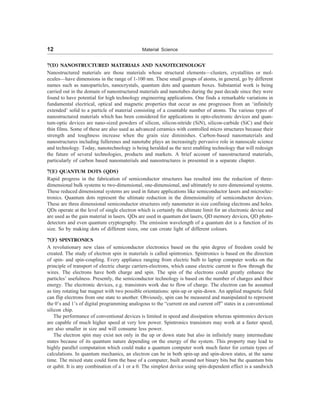
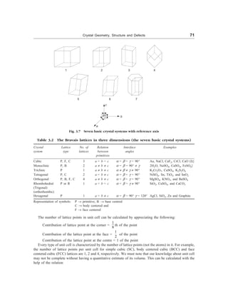
as phosphorus and arsenic which give it desired properties. Some simple defects in a lattice are shown in
Fig. 3.46.
There are some properties of materials such as stiffness, density and electrical conductivity which are
termed structure—insensitive, are not affected by the presence of defects in crystals while there are many
properties of greatest technical importance such as mechanical strength, ductility, crystal growth, magnetic](https://image.slidesharecdn.com/s-230301071329-4f25d7e9/85/S-L-_Kakani-_Material_Science_-New_Age_Pub-_2006-BookSee-org-pdf-112-320.jpg)
![96 Material Science
b
a
d
e
c
key:
a = vacancy (Schottky defect)
b = interstitial
c = vacancy—interstitial pair (Frenkel defect)
d = divacancy
e = split interstitial
= vacant site
Fig. 3.46 Some simple defects in a lattice
hysteresis, dielectric strength, condition in semiconductors, which are termed structure sensitive are greatly
affected by the relatively minor changes in crystal structure caused by defects or imperfections. Crystalline
defects can be classified on the basis of their geometry as follows:
(i) Point imperfections
(ii) Line imperfections
(iii) Surface and grain boundary imperfections
(iv) Volume imperfections
The dimensions of a point defect are close to those of an interatomic space. With linear defects, their
length is several orders of magnitude greater than the width. Surface defects have a small depth, while their
width and length may be several orders larger. Volume defects (pores and cracks) may have substantial
dimensions in all measurements, i.e. at least a few tens of Å. We will discuss only the first three crystalline
imperfections.
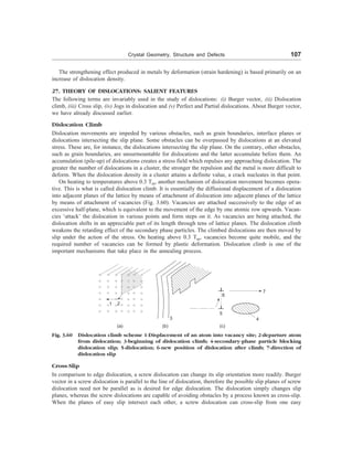
20. POINT IMPERFECTIONS
The point imperfections, which are lattice errors at isolated lattice points, take place due to imperfect
packing of atoms during crystallisation. The point imperfections also take place due to vibrations of atoms
at high temperatures. Point imperfections are completely local in effect, e.g. a vacant lattice site. Point
defects are always present in crystals and their present results in a decrease in the free energy. One can
compute the number of defects at equilibrium concentration at a certain temperature as,
n = N exp
d
E
kT
-
é ù
ê ú
ë û
(8)
Where n ® number of imperfections, N ® number of atomic sites per mole, k ® Boltzmann constant,
Ed ® free energy required to form the defect and T ® absolute temperature. E is typically of order l eV;
since k = 8.62 ´ 10–5
eV/K, at T = 1000 K, n/N = exp[–1/(8.62 ´ 10–5
´ 1000)] ; 10–5
, or 10 parts per
million. For many purposes, this fraction would be intolerably large, although this number may be reduced
by slowly cooling the sample.
(i) Vacancies: The simplest point defect is a vacancy. This refers to an empty (unoccupied) site of a crystal
lattice, i.e. a missing atom or vacant atomic site [Fig. 3.47(a)] such defects may arise either from imperfect
packing during original crystallisation or from thermal vibrations of the atoms at higher temperatures. In
the latter case, when the thermal energy due to vibration is increased, there is always an increased prob-
ability that individual atoms will jump out of their positions of lowest energy. Each temperature has a](https://image.slidesharecdn.com/s-230301071329-4f25d7e9/85/S-L-_Kakani-_Material_Science_-New_Age_Pub-_2006-BookSee-org-pdf-113-320.jpg)
![Crystal Geometry, Structure and Defects 97
(a) Vacancy defect (b) Interstitial defect
(c) Frenkel defect (d) Substitutional defect
(e) Schottky defect
Fig. 3.47 Point defects in a crystal lattice
corresponding equilibrium concentration of vacancies and interstitial atoms (an interstitial atom is an atom
transferred from a site into an interstitial position). For instance, copper can contain 10–13
atomic percentage
of vacancies at a temperature of 20–25°C and as many as 0.01% at near the melting point (one vacancy
per 104
atoms). For most crystals the said thermal energy is of the order of l eV per vacancy. The thermal
vibrations of atoms increases with the rise in temperature. The vacancies may be single or two or more of
them may condense into a di-vacancy or trivacancy. We must note that the atoms surrounding a vacancy
tend to be closer together, thereby distorting the lattice planes. At thermal equilibrium, vacancies exist in
a certain proportion in a crystal and thereby leading to an increase in randomness of the structure. At higher
temperatures, vacancies have a higher concentration and can move from one site to another more frequently.
Vacancies are the most important kind of point defects; they accelerate all processes associated with
displacements of atoms: diffusion, powder sintering, etc.
(ii) Interstitial Imperfections: In a closed packed structure of atoms in a crystal if the atomic packing factor
is low, an extra atom may be lodged within the crystal structure. This is known as interstitial position, i.e.
voids. An extra atom can enter the interstitial space or void between the regularly positioned atoms only
when it is substantially smaller than the parent atoms [Fig. 3.47(b)], otherwise it will produce atomic
distortion. The defect caused is known as interstitial defect. In close packed structures, e.g. FCC and HCP,
the largest size of an atom that can fit in the interstitial void or space have a radius about 22.5% of the
radii of parent atoms. Interstitialcies may also be single interstitial, di-interstitials, and tri-interstitials. We
must note that vacancy and interstitialcy are inverse phenomena.](https://image.slidesharecdn.com/s-230301071329-4f25d7e9/85/S-L-_Kakani-_Material_Science_-New_Age_Pub-_2006-BookSee-org-pdf-114-320.jpg)
![98 Material Science
(iii) Frenkel Defect: Whenever a missing atom, which is responsible for vacancy occupies an interstitial site
(responsible for interstitial defect) as shown in Fig. 3.47(c), the defect caused is known as Frenkel defect.
Obviously, Frenkel defect is a combination of vacancy and interstitial defects. These defects are less in
number because energy is required to force an ion into new position. This type of imperfection is more
common in ionic crystals, because the positive ions, being smaller in size, get lodged easily in the interstitial
positions.
(iv) Schottky Defect: These imperfections are similar to vacancies. This defect is caused, whenever a pair
of positive and negative ions is missing from a crystal [Fig. 3.47(e)]. This type of imperfection maintains
a charge neutrality. Closed-packed structures have fewer interstitialcies and Frenkel defects than vacancies
and Schottky defects, as additional energy is required to force the atoms in their new positions.
(v) Substitutional Defect: Whenever a foreign atom replaces the parent atom of the lattice and thus occupies
the position of parent atom (Fig. 3.47(d)], the defect caused is called substitutional defect. In this type of
defect, the atom which replaces the parent atom may be of same size or slightly smaller or greater than that
of parent atom.
(vi) Phonon: When the temperature is raised, thermal vibrations takes place. This results in the defect of
a symmetry and deviation in shape of atoms. This defect has much effect on the magnetic and electric
properties.
All kinds of point defects distort the crystal lattice and have a certain influence on the physical prop-
erties. In commercially pure metals, point defects, increase the electric resistance and have almost no effect
on the mechanical properties. Only at high concentrations of defects in irradiated metals, the ductility and
other properties are reduced noticeably.
In addition to point defects created by thermal fluctuations, point defects may also be created by other
means. One method of producing an excess number of point defects at a given temperature is by quenching
(quick cooling) from a higher temperature. Another method of creating excess defects is by severe defor-
mation of the crystal lattice, e.g., by hammering or rolling. We must note that the lattice still retains its
general crystalline nature, numerous defects are introduced. There is also a method of creating excess point
defects is by external bombardment by atoms or high energy particles, e.g. from the beam of the cyclotron
or the neutrons in a nuclear reactor. The first particle collides with the lattice atoms and displaces them,
thereby causing a point defect. The number of point defects created in this manner depends only upon the
nature of the crystal and on the bombarding particles and not on the temperature.
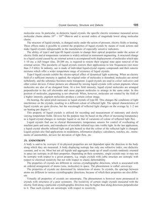
21. LINE DEFECTS OR DISLOCATIONS
Line imperfections are called dislocations. A linear disturbance, i.e. one dimensional imperfections in the
geometrical sense of the atomic arrangement, which can very easily occur on the slip plane through the
crystal, is known as dislocation. The most important kinds of linear defects are edge and screw dislocation.
Both these types are formed in the process of their deformation. Both these defects are the most striking
imperfections and are responsible for the useful property of ductility in metals, ceramics and crystalline
polymers.
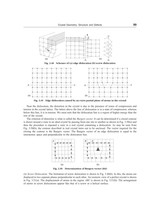
(i) Edge Dislocation: This type of dislocation is formed by adding an extra partial plane of atoms to the
crystal [Fig. 3.48(a)]. An edge dislocation in its cross-section is essentially the edge of an ‘extra’ half-plane
in the crystal lattice. The lattice around dislocation is elastically distorted.
Figure 3.49(a) shows a cross-section of a crystal where atoms (shown by dots) arranged in a perfect
orderly manner. When an extra half plane is inserted from the top, the displacement of atoms is shown in
Fig. 3.49(b). We note from Fig. 3.49(b) that top and bottom of the crystal above and below the line XY
appears perfect. When the extra half plane is inserted from the top, the defects so produced is represented
by ^ (inverted tee) and if the extra half plane is inserted from the bottom, the defects so produced is
represented by T (Tee).](https://image.slidesharecdn.com/s-230301071329-4f25d7e9/85/S-L-_Kakani-_Material_Science_-New_Age_Pub-_2006-BookSee-org-pdf-115-320.jpg)
![102 Material Science
Boundary
Grain I Grain II
d a
a
(a) (b)
Fig. 3.54 Schemes of (a) high angle and (b) low-angle boundaries
The lower atomic packing along the boundary favours
atomic diffusion. When the orientation difference between
neighbouring grains is more than 10°–15°, boundaries are
called high angle grain boundaries (Fig. 3.54(a)). Each
grain in turn consists of subgrains or blocks.
A subgrain is a portion of a crystal of a relatively regular
structure. Subgrain boundaries are formed by walls of dis-
locations which divide a grain into a number of subgrains
or blocks [Fig. 3.54(b)]. Angle of misorientation between
adjacent subgrains are not large (not more than 5°), so that
their boundaries are termed ‘low angle’. Low angle bound-
aries can also serve as places of accumulation of impurities.
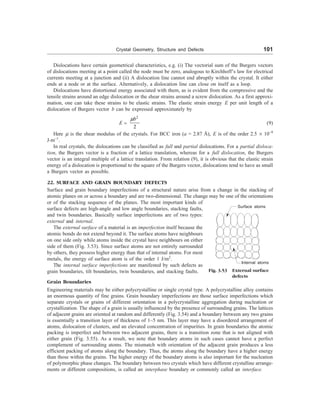
Tilt Boundaries
This is another type of surface defect called low-angle
boundary as the orientation difference between two neigh-
bouring crystals is less than 10°. This is why the disruption
in the boundary is not so drastic as in the high angle bound-
ary. This type of boundary is associated with relatively
little energy and is composed of edge dislocations lying one
above the other. In general, one can describe low-angle
boundaries by suitable arrays of dislocation. The angle or
tilt, q =
b
D
[Fig. 3.55(a)], where b is the magnitude of
Burgers vector and B is the average vertical distance be-
tween dislocations.
Twin Boundaries
Grain boundary
Fig. 3.55 Area of disorder at grain boun-
daries
Boundary
Grain 2
b
D =
q
b
Grain 1
q
Fig. 3.55(a) Tilt boundary
This is another planar surface imperfection. The atomic arrangement on one side of a twin boundary is a
mirror reflection of the arrangement on the other side. Twinning may result during crystal growth or
deformation of materials. Twin boundaries occur in pairs, such that the orientation change introduced by
one boundary is restored by the other. The region between the pair of boundaries is termed as the twinned
region. One can easily identify twin boundaries under an optical microscope. Twins which form during the
process of recrystallization, i.e., in the process of mechanical working are known as mechanical twins,
whereas twins formed as a result of annealing after plastic deformation are known as annealing twins
(Fig. 3.56).](https://image.slidesharecdn.com/s-230301071329-4f25d7e9/85/S-L-_Kakani-_Material_Science_-New_Age_Pub-_2006-BookSee-org-pdf-119-320.jpg)
![106 Material Science
Magnetic properties are found to be anisotropic in cubic crystals as well. For instance, the magnetization
of ferromagnetics with a cubic lattice is different in various crystallographic directions. For a-Fe (BCC
lattice), the direction of easy magnetization is [100], for Ni (FCC lattice), it is [111], and for Co (HCP
lattice), it is [110].
Examples of bodies which are anisotropic in some of their properties are liquid ‘crystals’, single crystals,
and aggregates of polycrystals with a preferred orientation.
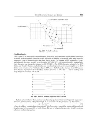
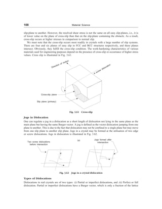
26. FRANK-READ SOURCE
It is observed that slip occurs intensely on a small number of crystal planes and, during the process, some
hundreds of dislocations move. Obviously, there must be some effective creators or some mechanisms by
which these numerous dislocations are produced on a given slip plane. These are called as Frank-Read
sources. A single Frank-Read dislocation source can form hundreds of new dislocations.
It is observed in practical tests that under relatively high stresses, the incidence of plastic deformation
is high in most metals through the combined movement of many hundred thousand of dislocations in
individual crystals. Plastic deformation in real crystals is effected by successive movements of dislocations.
Frank-Read mechanism helps to explain the existence of so called dislocation mills or multiplication of
dislocations (Fig. 3.59). Let us consider a dislocation line, shown by AB in a crystal. We see that the
dislocation line or Frank-Read source consists of two nodes A and B. In the first situation, when the Burger
vector is perpendicular to the line AB, a shear stress parallel to the plane of the figure will exert a force
on the dislocation line AB. Due to the action of the shear stress the dislocation line bent outward and
produces slip. A slip plane usually contains tens of dislocations. For a given stress, the dislocation line AB
assume a certain radius of curvature. On further increasing the stress, the dislocation line becomes unstable
and expands indefinitely. Figure 3.59 illustrates the successive stages.
A B
(a)
A B
(b)
A B
A B
(d)
A B
(e)
(c)
Fig. 3.59 Sequence of formation of a new dislocation by Frank-Read source. A dislocation is pinned by
two pinning sites. Under the action of the applied shear stress a fixed (sessile) dislocation is
bent outward until it becomes hemispherical. From that moment on, the dislocation will
spontaneously pass through the configurations as shown in figure and a dislocation loop will
be generated
Under the action of the applied stress, the fixed dislocation line AB is bent outward until it becomes
hemispherical (Fig. 3.59(a) and (b)) of radius AB/2. We must note that if the stress is removed at any stage
upto this point AB will regain its original shape. If the stress is further increased to the stage (Fig. 3 59(c))
at which the bulge becomes greater than a semicircle, a new system of balance exists and a lower strain
energy will be attained by the loop becoming larger (i.e., radius of loop increasing again). From that
moment on, the bent dislocation propagates spontaneously in the form of two spirals. As the spirals meet,
they give rise to an expanding dislocation loop and a dislocation section. The dislocation section occupies
an initial position and the dislocation source is ready to repeat the cycle. A single Frank-Read dislocation
source can form hundreds of new dislocations.](https://image.slidesharecdn.com/s-230301071329-4f25d7e9/85/S-L-_Kakani-_Material_Science_-New_Age_Pub-_2006-BookSee-org-pdf-123-320.jpg)
![Crystal Geometry, Structure and Defects 109
translation vector. Partial dislocation is always associated with a surface imperfection or fault in the stack-
ing arrangement of planes in the crystal. Perfect or full dislocations are surrounded by good regions of the
crystal, i.e., on both the sides of the dislocation, the vertical planes match across the slip plane. This is
possible because the Burger vector of perfect or full dislocation is an integral multiple of the lattice
translation vector.
Example 20 Calculate the line energy of dislocations in BCC iron. Given, the Burgers vector in iron is
of the
1
2
111 type and shear modulus of iron is 80.2 GN/m2
[BE]
Solution For BCC iron, the lattice parameter, a = 2.87 Å. Magnitude of Burgers vector,
b = 2.87 3 2 = 2.49 Å.
We have the relation for the line energy of the dislocation,
E ; 1
2
mb2
=
9 2 20
80.2 10 (2.49) 10
2
-
´ ´ ´
= 2.49 ´ 10–9
J/m.
Example 21 A circular dislocation loop has edge character all round the loop. Show that the surface
on which this dislocation can glide should be a cylindrical surface containing the loop.
[M.Sc. (MS), AMIE]
Solution We know that the Burgers vector (b
®
) is perpendicular to an edge dislocation line and Burgers
vector is invariant. We also know that the edge dislocation can glide only on a surface which contains both
the Burgers vector (b
®
) and the direction vector ( t
®
). These considerations are satisfied only when the
dislocations moves, i.e. glide, on a cylindrical surface containing the loop.
Example 22 There are 1010
m–2
of edge dislocations in a simple cubic crystal. How much would each
of these climb down on an average, when the crystal is heated from 0 to 1000 K. Given, the lattice
parameter = 2 Å, volume of 1 mole of the crystal is 5.5 ´ 10–6
m3
(= 5.5 cm3
) and the enthalpy of formation
of vacancies is 100 kJ/mol. [BE]
Solution We know that at equilibrium, there are no vacancies in the crystal at 0 K. Now, to maintain the
equilibrium concentration, the number of vacancies that must be created on heating from 0 to 1000 K is
given by
n = N exp
f
H
RT
- D
é ù
ê ú
ë û
Substituting the proper values in the above relation, one obtains
n = 6.023 ´ 1023
exp
100 1000
8.314 1000
´
é ù
-
ê ú
´
ë û
= 3.6 ´ 1018
/mol. = 6.54 ´ 1023
m–3
Example 23 The surface of a copper crystal is of the {111} type. Show that the surface energy, i.e.
enthalpy of copper is about 2.49 J-m–2
.
Solution We have the bond energy per atom of copper
= bond energy per bond ´ no. of bonds per atom ´
1
2](https://image.slidesharecdn.com/s-230301071329-4f25d7e9/85/S-L-_Kakani-_Material_Science_-New_Age_Pub-_2006-BookSee-org-pdf-126-320.jpg)
![110 Material Science
=
23
56.4 1000 12
6.023 10 2
´ ´
´ ´
= 5.62 ´ 10–19
J
Out of the twelve bonds, three bonds are broken at the surface. Energy of broken bonds per atom
= 5.62 ´ 10–19
´
1
4
J
Number of atoms on {111} planes in copper
= 1.77 ´ 10–19
m–2
Surface energy (enthalpy) of copper
= 5.62 ´ 10–19
´
1
4
´ 1.77 ´ 1019
= 2.49 J/m2
(= 2490 erg/cm2
)
Example 24 Find the equilibrium concentration of vacancies in aluminium at 0 K and 300 K.
[AMIE]
Solution For Aluminium DHf = 68 kJ mol–1
and
vacancy
eV
= 0.70
we have
n
N
= exp
f
H
RT
D
é ù
-
ê ú
ë û
(i) At 0 K,
n
N
= exp
3
68 10
8.314 0
é ù
´
-
ê ú
´
ë û
= exp(–¥) = 0
(ii) At 300 K
n
N
= exp
3
68 10
8.314 300
é ù
´
-
ê ú
´
ë û
= exp(–27.26)
= 10
27.26
2.303
-
= 10–11.84
Log
n
N
= –11.84
n
N
= 1.45 ´ 10–12
28. DETERMINATION OF CRYSTAL STRUCTURE BY X-RAY DIFFRACTION
X-rays provide a powerful tool for the study of crystal structure. X-rays, being electromagnetic radiations,
also undergo the phenomenon of diffraction as observed for visible light. The ordered arrangement of atoms
in a crystal with interatomic spacing of the order of few angstroms behaves like a three-dimensional
diffraction grating for X-rays. One can easily verify this. Let us consider sodium metal whose density r and
molecular weight, M are 1.013 ´ 103
kg/m3
and 23 respectively. The structure of sodium is BCC and
number of atoms/unit volume = Nr/M = 2/a3
, where N is Avogadro number (= 6.023 ´ 1026
) and a is cell
constant. So, we have
a =
1/3
1/3
26 3
2 23
2
6.023 10 1.013 10
M
Nr
´
é ù
æ ö = ê ú
ç ÷
è ø ´ ´ ´
ë û
= 4.225 Å](https://image.slidesharecdn.com/s-230301071329-4f25d7e9/85/S-L-_Kakani-_Material_Science_-New_Age_Pub-_2006-BookSee-org-pdf-127-320.jpg)
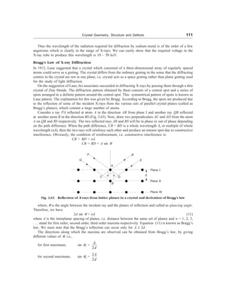
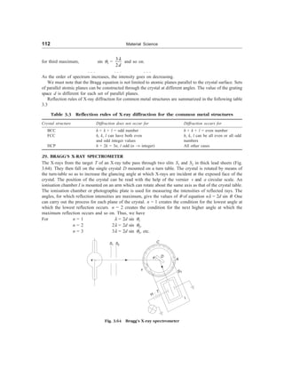
![Crystal Geometry, Structure and Defects 113
A1
A2
A3
1
where q1, q2 and q3 are glancing angles for n = 1, 2 and 3 respectively. Thus
sin q1 : sin q2 : sin q3 = 1 : 2 : 3 (12)
Obviously, by measuring glancing angles at which reflection occurs, one can determine the interplanar
spacings knowing the wavelength of X-rays.
The variation of ionization current against glancing angle q is shown in Fig. 3.65. This curve is obtained
when X-rays from a tube containing a platinum target were reflected by a crystal of rock salt (NaCl).
The experimental results have shown that the first order reflection maxima occurred at 5.9°, 8.4° and
5.2° for (100), (110) and (111) planes respectively.
For first order reflection, n = 1 and hence
d =
2sin
l
q
or d µ
1
sinq
d100 : d110 : d111 =
1 2 3
1 1 1
: :
sin sin sin
q q q
or d100 : d110 : d111 =
1 1 1
: :
sin 5.9 sin 8.4 sin 5.2
° ° °
= 9.73 : 6.84 : 11.04
d100 : d110 : d111 = 1 :
1 2
:
2 3
One can follow this procedure for other crystals. Following table summarizes the values of ratios between
interplanar distance of planes (100), (110) and (111) for the cubic structures.
Table 3.4 Ratio between interplanar distances
S. No. Type of cubic structure
100
1
d
:
110
1
d
:
111
1
d
1 Simple cubic 1 : 2 : 3
2 BCC 1 :
1
2
: 3
3 FCC 1 : 2 :
3
2
Example 25 Determine the interplanar spacing when a beam of X-ray of wavelength 1.54 Å is directed
towards the crystal at angle 20.3° to the atomic plane. [AMIE]
Solution 2d sin q = nl l = 1.54 Å
2d sin 20.3° = 1 ´ 1.54 q = 20.3°
d =
1.54 1.54
2sin 20.3 2 0.3469
=
° ´
= 2.22 Å
Example 26 X-rays with wavelength of 0.58 Å are used for calculating d200 in nickel. The reflection angle
is 9.5°. What is the size of unit cell? [AMIE]
2 3
n =
incident angle
Fig. 3.65 Variation of ionization
current with glancing
angle
Ionization
current](https://image.slidesharecdn.com/s-230301071329-4f25d7e9/85/S-L-_Kakani-_Material_Science_-New_Age_Pub-_2006-BookSee-org-pdf-130-320.jpg)
![114 Material Science
Solution d =
2 2 2
a
h k l
+ +
l = 0.58 Å
q = 9.5°
d200 =
2 2 2 2
2 0 0
a a
=
+ +
= 0.5a
Now, from Bragg’s law
2d sin q = nl, we have
2 d200 sin 9.5° = 1 ´ 0.58
2 ´ 0.5a ´ 0.165 = 0.58
a =
0.58
1.165
= 0.52 Å
Example 27 Calculate the Bragg angle if (111) planes of a cube (a = 3.57 Å) crystal are exposed to
X-rays (wavelength = 1.54 Å) [AMIE]
Solution We have, Miller indices of the (111) planes, h = 1, k = 1 and l = 1; a = 3.57° and l = 1.54 Å.
Let q be the Bragg’s angle for the first order reflection.
We have d =
2 2 2
a
h k l
+ +
d111 =
2 2 2
3.57
(1) (1) (1)
+ +
= 2.06 Å
Now, from Bragg’s law, we have
2d111 sin q = nl
2 ´ 2.06 ´ sin q = 1 ´ 0.54
sin q =
1 0.54
2 2.06
´
´
= 0.131
q = 7° 32¢
Example 28 For a certain BCC crystal, the (110) plane has a separation of 1.181 Å. These planes are
indicated with X-ray of wavelength 1.540 Å. Show that the maximum order of the Bragg’s reflection that
can be observed is n = 1.
Solution 2d sin q = nl d = 1.181 Å
l = 1.540 Å
n =
2 sin
d q
l
=
2 1.181sin 90
1.540
´ °
= 1.53
Since the value of ‘n’ can be integer only, and hence the highest possible value of n in this case is 1.
Example 29 The glancing angle of 10° is observed in first order Bragg’s reflection. Show that the angle
for 3rd order reflection is 31.39°.
Solution For n = 1, q1 = 10°
For n = 3, q3 = ?](https://image.slidesharecdn.com/s-230301071329-4f25d7e9/85/S-L-_Kakani-_Material_Science_-New_Age_Pub-_2006-BookSee-org-pdf-131-320.jpg)
![Crystal Geometry, Structure and Defects 115
l = 2 Å
q = 30°
n = 1
h = k = l = 1
From Bragg’s law, we have
2d sin q1 = 1l (First order)
2d sin q3 = 3l (Third order)
1
3
sin
sin
q
q
=
1
3
or sin q3 = 3 sin q1 = 3 ´ sin 10° = 3 ´ 0.1736 = 0.5209
q3 = 31.39°.
Example 30 A diffraction pattern of a cubic crystal of lattice parameter a = 3.16 Å is obtained with a
monochromatic X-ray beam of wavelength 1.54 Å. The first line on this pattern was observed to have
q = 20.3°. Obtain the interplanar spacing and Miller indices of the reflecting plane.
[B.E.; B.Sc. (Hons.)]
Solution 2d sin q = nl
d =
2sin
nl
q
=
1 1.54
2 0.3469
´
´
= 2.22 Å
For cubic crystal, we have
d =
2 2 2
a
h k l
+ +
or h2
+ k2
+ l2
=
2
2
2 2
(3.16)
(2.22)
a
d
= = 2
Since (h2
+ k2
+ l2
) = 2 and hence the Miller indices are (110) or (101) or (011).
Example 31 Determine interatomic spacing when glancing angle of 30° is observed during first order
reflection in a crystal having Miller indices as (111). The wavelength of X-rays is 2 Å.
Solution d =
2 2 2
a
h k l
+ +
d =
2 2 2 3
(1) (1) (1)
a a
=
+ +
Now, 2d sin q = nl
2
3
a
sin 30° = 1 ´ 2 Å
a = 2 3 Å
30. RECIPROCAL LATTICE
We have seen that the diffraction of X-rays occurs from various sets of parallel planes having different
orientations (slopes) and interplanar spacings. In certain situations involving the presence of a number of
q = 20.3°
l = 1.54 Å
n = 1
a = 3.16 Å](https://image.slidesharecdn.com/s-230301071329-4f25d7e9/85/S-L-_Kakani-_Material_Science_-New_Age_Pub-_2006-BookSee-org-pdf-132-320.jpg)
![116 Material Science
sets of parallel planes with different orientations, it becomes difficult to visualize all such planes because
of their two-dimensional nature. To solve the problem, Ewald introduced the new type of lattice known as
the reciprocal lattice. The idea underlying the development was that each set of parallel planes could be
represented by a normal to these planes having length equal to the reciprocal of the interplanar spacing.
Thus the direction of each normal represents the orientation of the corresponding set of parallel planes and
its length is proportional to the reciprocal of the interplanar spacing.
The normals are drawn with reference to an arbitrary origin and points are marked at their ends. These
points form a regular arrangement which is called a reciprocal lattice. Obviously, each point in a reciprocal
lattice is a representative point of a particular parallel set of planes and it becomes easier to deal with such
points than with sets of planes.
One can construct a reciprocal lattice to a direct lattice using the following procedure:
(i) Take origin at some arbitrary point and draw normals to every set of parallel planes of the direct
lattice
(ii) Take length of each normal equal to the reciprocal of the interplanar spacing for the corresponding
set of planes. The terminal points of these normals form the reciprocal lattice
Let us consider, as an example for the construction of reciprocal lattice, the unit cell of a monoclinic
crystal (a ¹ b ¹ c; a = b = 90° ¹ g) looking along its unique axis, i.e. c-axis. For simplicity, we may
consider planes belonging to a single zone. This makes the normal to all parallel planes belonging to the
zone axis, i.e., normal to the c-axis. In Fig. 3.66, we can see that the zone axis lies perpendicular to the
plane of the diagram and hence all normals to the parallel planes of the family of the zone will lie in the
plane of the diagram. Figure 3.66 also shows the edge views of four (h k l) planes, viz., (100), (110), (120)
and (010) all belonging to [001] zone. We must note that the normals to the family of planes (100), (200),
(300) etc. are parallel. Further d100 = 2d200 = 3d300 = 4d400 etc.
Obviously, while
s100 = k (1/d100),
s200 = 2s100;
s300 = 3s100 and
so. Clearly, the distance of the reciprocal lattice point representing the set of parallel planes (nh 00) from
the origin will be n times greater than the distance of the reciprocal lattice point from the origin representing
Fig. 3.66 Graphical construction of a two-dimensional reciprocal lattice
040
030
(110)
020
b 010
(120)
(010) c a
(100)
100
200
300
110
210
120
220
230](https://image.slidesharecdn.com/s-230301071329-4f25d7e9/85/S-L-_Kakani-_Material_Science_-New_Age_Pub-_2006-BookSee-org-pdf-133-320.jpg)
![Crystal Geometry, Structure and Defects 117
the set of parallel planes (300) will be at a distance from the origin equal to three times the distance of the
reciprocal lattice point representing the set of parallel planes (100). In reciprocal lattice, it is the convention
to represent the reciprocal lattice point representing the set of parallel planes with Miller indices (h, k l)
by the same Miller indices without the parenthesis. We can see in Fig. 3.66 that the reciprocal lattice points
representing the set of parallel planes (100), (200), (300) etc . . ., are indicated by 100, 200, 300 etc . .
. . As stated earlier, all the set of parallel planes (100), (200), (300) etc., have common normal all the
reciprocal lattice points 100, 200, 300 etc. all lie along the same straight line. We have taken the planes
belonging to [001] zone and after plotting the reciprocal lattice points of all the (h k o) planes, we obtained
a two dimensional lattice (Fig. 3.66). Ewald provided a vector-algebraic proof that a three-dimensional
reciprocal lattice is similarly formed in real crystal.
A reciprocal lattice vector, shkl, is defined as a vector having magnitude equal to the reciprocal of the
interplanar spacing dhkl and direction conciding with normal to (h k l) planes. Thus, we have
shkl =
1 ˆ
hkl
n
d
(13)
where n̂ is the unit vector normal to the (h k l) planes.
Denoting the fundamental reciprocal vector s100, s010 and s001 by a*, b* and c* respectively, one obtains
*
a
®
= s100 =
b c
a b c
® ®
®
® ®
´
× ´
b* = s010 =
c a
a b c
® ®
®
® ®
´
× ´
c* = s001 =
a b
a b c
® ®
®
® ®
´
× ´
(14)
where a
®
× b
®
´ c
®
= b
®
× c
®
´ a
®
= c
®
× a
®
´ b
®
is the volume of the direct cell. Obviously, the reciprocal
translation vectors bear a simple relationship to the crystal translation vectors as
a
®
* is normal to b
®
and c
®
b
®
* is normal to c
®
and a
®
(15)
c
®
* is normal to a
®
and b
®
In literature, sometime the primitive translation vectors a
®
, b
®
and c
®
of a direct lattice are related to the
primitive translation vectors a
®
*, b
®
* and c
®
* of the reciprocal lattice as
a
®
* = 2p
b c
a b c
® ®
®
® ®
´
× ´
b
®
* = 2p
c a
a b c
® ®
®
® ®
´
× ´
(16)
c
®
* = 2p
a b
a b c
®
®
®
® ®
´
× ´
ù
ú
ú
ú
û
ù
ú
ú
ú
ú
ú
ú
ú
ú
ú
ú
ú
ú
û](https://image.slidesharecdn.com/s-230301071329-4f25d7e9/85/S-L-_Kakani-_Material_Science_-New_Age_Pub-_2006-BookSee-org-pdf-134-320.jpg)
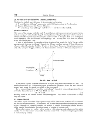
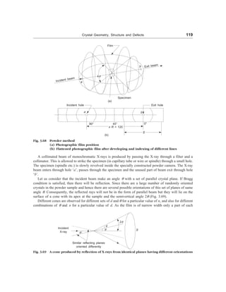
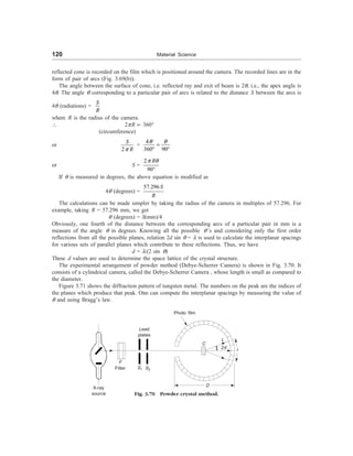
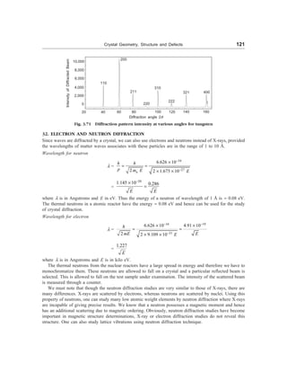
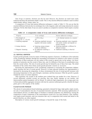
![Crystal Geometry, Structure and Defects 123
SUGGESTED READINGS
1. S.L. Kakani and C. Hemrajani, Solid State Physics (4th ed., 2004) Sultan Chand, New Delhi-2.
2. C. Kittel, Introduction to Solid State Physics, John Wiley, (7th ed.).
3. R.C. Evans, An Introduction to Crystal Chemistry, Cambridge Univ. Press (1964).
4. P.J. Brown and J.E. Forsyth, The Crystal Structure of Solids (1973).
5. F.C. Phillips, Introduction to crystallography, 4th ed. (1979).
6. J.H. Crawford. Jr. and L.M. Slifkin (eds.) Point Defects in Solids, vol. 1, 2 and 3 (1972, 75, 78).
7. B.D. Cullity and S.R. Stock, Elements of X-ray Diffraction, 3rd ed., Prentice Hall, Upper Saddle
River, NJ (2001).
8. D. Brandon and W.D. Kaplan, ‘Microstructural Characterization of Materials’, Wiley, New York,
(1999).
REVIEW QUESTIONS
1. Explain the concepts of lattice, basis and crystal structure. How are they related?
2. Draw primitive cells corresponding to BCC and FCC unit cells.
3. Describe, how atoms are arranged in cubic crystal?
4. What is Bravais lattice? What is the maximum number of Bravais lattices possible? How will you
account for the existence of thousands of structures from these lattices?
5. Write a short note on space lattice. [AMIE]
6. Draw net sketches of unit cells of simple cubic, BCC and FCC crystal structures. Calculate the
number of atoms in each case. [AMIE]
7. The end-centred orthorhombic is one of the Bravais lattices but the end-centred tetragonal is not. Give
reasons.
8. What is the number of atoms per unit cell in the FCC structure? [AMIE]
9. Give a brief account of crystal directions and crystallographic planes.
10. Draw the following:
(i) [111], [121] and [012] directions in cubic and tetragonal lattices.
(ii) [111], [112] and [210] planes in cubic and orthorhombic lattices.
11. Prove that in a cubic lattice the direction [hkl] is perpendicular to the plane (h k l).
12. Calculate the atomic packing factor of simple cubic, BCC and FCC crystals. [B.E.]
13. Draw a hexagonal closed packed unit cell. Calculate the number of atoms per unit cell. Calculate its
atomic packing factor.
14. Draw a plan view of sodium chloride structure. In how many ways can this structure be interpreted?
15. Write the points of similarity and differences of the monoatomic SC, monoatomic BCC and CsCl
structure.
16. What are Miller indices? How are they determined? [AMIE]
17. Draw atomic arrangement in planar surface imperfection with a boundary. [AMIE]
18. Discuss in brief the point defects. How these defect affect the properties of materials? [BE]
19. Explain Schottky and stacking faults.
20. Explain Miller Bravais system? How is this system used to find the index of different planes?
21. Using net sketches show (a) vacancy defect and interstitial defect in crystal. [AMIE]
22. State and explain the Bragg’s law of X-ray diffraction. What are its uses? [AMIE]
23. Discuss Bragg’s law of X-ray diffraction. Describe how the powder method is used for the determi-
nation of crystal structure. [AMIE]](https://image.slidesharecdn.com/s-230301071329-4f25d7e9/85/S-L-_Kakani-_Material_Science_-New_Age_Pub-_2006-BookSee-org-pdf-140-320.jpg)
![124 Material Science
24. Explain how with the help of X-ray diffraction techniques, the lattice dimensions are determined.
25. Write the different diffraction methods of determining crystal structure and describe any one in detail.
26. Write short notes on
(i) Bravais Lattices (ii) Coordination number
(iii) Crystal defects (iv) Crystal growth
(v) Crystal Whiskers (vi) Grain boundaries
(vii) Crystallographic indices (viii) Liquid crystals
(xi) Bragg’s law (x) X-ray spectrometer
(xi) Electron and neutron diffraction
PROBLEMS
1. Draw a (110) plane in a cubic unit cell. Show all the 111 directions that lie on this plane and give
the Miller indices of each direction. ([111], [111], [1 11] and [1 1 1])
2. A plane makes intercepts of 1, 2 and 3 Å on the crystallographic axes of an orthorhombic crystal with
a : b : c = 3 : 2 : 1. Determine the Miller indices of this plane (9 3 1)
3. Aluminium has an FCC structure. Its density is 2700 kg/m3
(sp. gravity = 2.7). Find the unit cell
dimension and the atomic diameter. [4.05Å, 2.86 Å]
4. Show that the shortest centre to centre distance between any two atoms among the four atoms located
inside the diamond-cubic unit cell is 2
a .
5. Determine the number of the nearest neighbours and the closest distance of approach in terms of
lattice parameter for monoatomic SC, BCC and FCC structures. [6, a; 8, 3/2
a ; 12, / 2
a ]
6. Prove that c/a ratio for an ideal HCP structure is 1.633.
7. Zinc (HCP) has lattice parameters a and c as 2.66 Å and 4.95 Å respectively. Calculate the packing
fraction and density of zinc, given the atomic radius and the atomic mass of Zn as 1.31 Å and 65.37
amu respectively. [62%, 7155 kg-m–3
]
8. Calculate the density of CsCl crystal. Given radii of Cs+
= 1.65 Å and Cl–
= 1.81 Å
[4380 kg-m–3
]
9. A crystal plane makes intercepts 4a, 2b and –2c on the crystallographic axes of a crystal whose unit
cell has dimensions a, b and c. Find the Miller indices of the plane. [(122)]
10. The grating space for the (100) plane in a cubic crystal is found to be 2.84 ´ 10–10
m. Calculate the
grating space for the (100) and (111) planes. [2.008 ´ 10–10
m, 1.603 ´ 10–10
m]
11. Show that the maximum occupied volumes by hard spheres arranged in the structures given below are:
Simple cubic p/6
FCC p 21/2
/6
Diamond p 31/2
/16
12. Copper (FCC) has density of 8960 kg-m–3
. Calculate the unit cell dimension and radius of Cu atom,
given the atomic mass of Cu = 63.54 amu. [3.61Å, 1.28 Å]
13. A crystal reflects monochromatic X-rays strongly when the Bragg’s glancing angle for a first order
reflection is 15°. Show that the glancing angles for the second and third order reflections of the same
type are 31.2° and 50.9° respectively.
14. Copper (FCC) has a lattice parameter of 3.61Å. The first order Bragg reflection from (111) planes
appears at an angle 21.7°. Show that the wavelength of X-rays used is 1.54 Å.
15. An aluminium crystal has dislocation density of 1010
m–2
. The shear modulus of aluminium is 25.94
GN-m–2
. Show that the elastic energy of line imperfections stored in the crystal is 10.6 J-m–3
.
16. Calculate the spacing between dislocations in a tilt boundary in FCC nickel. Given, the angle of tilt
is 2°. [71.3 Å], [B.E.]](https://image.slidesharecdn.com/s-230301071329-4f25d7e9/85/S-L-_Kakani-_Material_Science_-New_Age_Pub-_2006-BookSee-org-pdf-141-320.jpg)
![Crystal Geometry, Structure and Defects 125
17. Calculate the dislocation energy per m3
of copper (FCC) with a dislocation density of 1010
m–2
.
Given, shear modulus of copper = 45 GN m–2
and lattice parameter = 3.61 Å [14.7 J-m–2
]
OBJECTIVE QUESTIONS
1. The number of lattice points in a primitive cell are
(1) 3/2 (2) 1/2 (3) 2 (4) 1 (4)
2. The number of lattice points in a rhombohedral unit cell is
(1) 1 (2) 2 (3) 4 (4) 16 (1)
3. The number of atoms present in the unit cell of HCP structure is
(1) 2 (2) 4 (3) 6 (4) 12 (3)
4. The minimum number of ions in the unit cell of an ionic crystal with FCC space lattice is
(1) 16 (2) 12 (3) 8 (4) 2 (3)
5. If r be the radius of the atom in a crystal crystallizing in the simple cubic structure, then the nearest
neighbour distance is
(1) 8r (2) 4r (3) 2r (4) r (3)
6. The space lattices with two lattice parameters does not belong to the crystal system
(1) triclinic (2) rhombohedral (3) hexagonal (4) tetragonal (1)
7. The number of diad axes of symmetry elements that are present in a cubic crystal are
(1) 6 (2) 3 (3) 2 (4) 1 (1)
8. The nearest neighbour distance in BCC structure is
(1) 2
a (2) 2 3
a (3) 3 2
a (4) 2 3
a (3)
9. The unit cell with three lattice parameter is
(1) monoclinic (2) tetragonal (3) triclinic (4) orthorhombic (3)
10. Which one of the following metals crystallizes in FCC structure
(1) zinc (2) sodium (3) aluminium (4) caesium chloride (3)
11. The atomic diameter of an FCC crystal (lattice parameters a) is
(1)
2
a
(2) 2
a (3)
2
2
a
(4)
2 2
a
(3)
12. The number of Bravais lattices with two lattice points are
(1) 5 (2) 6 (3) 3 (4) 1 (1)
13. The packing factor of diamond cubic crystal structure is
(1) 90% (2) 45% (3) 34% (4) none of these (4)
14. The unit cell has a = 5 Å, b = 8 Å, c = 3 Å, a = 90°, b = 65° and g = 54°. The space lattice for
this unit cell is
(1) monoclinic (2) rhombohedral (3) triclinic (4) orthorhombic (3)
15. The faces in a tetragon are
(1) 24 (2) 12 (3) 6 (4) 2 (2)
16. Magnesium crystallizes in HCP structure. If the lattice constant is 0.32 nm, the nearest neighbour
distance in magnesium is
(1) 0.64 nm (2) 0.32 nm (3) 0.16 nm (4) 0.8 nm (2)
17. Zinc crystallizes in HCP structure. If r is the radius of zinc atom, the height of the unit cell is
(1) 3/ 8
r (2) 2 8/ 3
r (3)
8
3
r (4) 2r (2)
18. The lattice constant of a BCC unit cell with atomic radius of 1.24 Å is
(1) 1.432 Å (2) 2.864 Å (3) 1.754 Å (4) 1.432 Å (2)](https://image.slidesharecdn.com/s-230301071329-4f25d7e9/85/S-L-_Kakani-_Material_Science_-New_Age_Pub-_2006-BookSee-org-pdf-142-320.jpg)
![126 Material Science
19. The correct order of coordination number in BCC, FCC and HCP unit cells is
(1) 12, 8, 6 (2) 8, 12, 12 (3) 6, 8, 12 (4) 12, 8, 24 (2)
20. The number of sulphide atoms in the unit cell of zinc sulphide crystal is
(1) 6 (2) 4 (3) 2 (4) 1 (2)
21. The Miller indices of the line of intersection of a (111) and a (110) plane are
(1) [110] (2) [111] (3) [1 10] (4) [110] (1, 3)
22. The Miller indices of the plane parallel to Y and Z axes are
(1) (0 0 1) (2) (1 1 1) (3) (0 1 0) (4) (1 0 0) (4)
23. The Miller indices of a plane in an orthorhombic unit cell (a : b : c = 1 : 2 : 3) making intercepts
of 3, 2, 1Å on a, b, c axes respectively are
(1) (1 2 3) (2) (3 2 1) (3) (9 3 1) (4) (1 3 9) (4)
24. If (3 2 6) are the Miller indices of a plane, the intercepts made by the plane on the three crystallo-
graphic axes are
(1) (a, b, c) (2) (2a, 3b, c) (3) (a, 2b, 3c) (4) (2a, b, 3c) (2)
25. In a simple cubic lattice d100 : d110 : d111 is
(1) 6 : 3 : 2 (2) 6 : 3 : 2 2
(3) 6 : 3 : 4 (4) 6: 3 : 2 (1)
26. THe acute angle between [101] and [101] directions in a tetragonal crystal with c/a = 1.5 is
(1) 67.38° (2) 45° (3) 33.69° (4) 90° (1)
27. The maximum radius of the interstitial sphere that can fit into the void between the body centred atom
of BCC structure is
(1) 3 1
r é ù
-
ë û (2) 2 1
r é ù
-
ë û (3) (2 3) 1
r é ù
-
ë û (4) 2
r (3)
28. The interplanar spacing of the first reflecting plane (lowest q) in an FCC crystal is
(1) 3
a (2) 2 3
a (3) a (4) 2 5
a (2)
29. A plane in a unit cell is described by its Miller indices (632). The plane intersects x, y, z respectively
at points whose distances from origin are
(1) 6, 3 and 2 units (2) 1/3, 2/3 and 1 units
(3) 1/3, 1/2 and 1/1 units (4) 1/6, 1/3 and 1/2 units (3)
30. If the first reflection from an FCC crystal has a Bragg angle q = 21.5°, the q corresponding to second
reflection is
(1) 13.5° (2) 18.5° (3) 25° (4) 36.8° (3)
31. The Miller indices of the fifth reflection in an FCC crystal is
(1) 111 (2) 222 (3) 311 (4) 331 (2)
32. The number of atoms per unit area of the plane (010) of a simple cubic crystal is
(1) 1/2r (2) 1/4r2
(3) 2r2
(4) 4r2
(2)
33. The highest linear density, i.e., the densest direction in FCC and BCC crystals are respectively
(1) 110 and 111 (2) 111 and 111
(3) 100 and 110 (4) 111 and 110 (1)
34. In a unit cell whose lattice constant is a, the distance between two {hkl} planes is
(1) 2 2 2
h k l
+ + (2) 2 2 2
a h k l
+ +
(3) 2 2 2
1 h k l
+ + (4) 2 2 2
hkl h k l
+ + (2)
35. No reflection will be observed from a DC crystal (a = 3Å), if the wavelength of X-rays is greater than
(1) 2.5 Å (2) 3.0 Å (3) 3.46 Å (4) 3.15 Å (3)](https://image.slidesharecdn.com/s-230301071329-4f25d7e9/85/S-L-_Kakani-_Material_Science_-New_Age_Pub-_2006-BookSee-org-pdf-143-320.jpg)
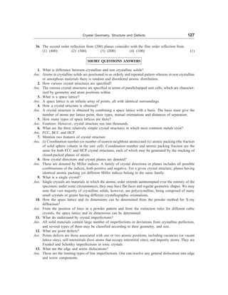
![128 Material Science
14. How a solid solution may be formed?
Ans. A solid solution may be formed when impurity atoms are added to a solid, in which case the original
crystal structure is retained and no new phases are formed.
15. What do you understand by substitutional solid solutions?
Ans. For substitutional solid solutions, impurity atoms substitute for host atoms, and appreciable solubility
is possible only when atomic diameters and electronegativities for both atom types are similar, when
both elements have the same crystal structure, and when the impurity atoms have a valence that is the
same as or less than the host material.
16. What are interstitial solid solutions?
Ans. These form for relatively small impurity atoms that occupy interstitial sites among the host atoms.
17. How the composition of an alloy may be specified?
Ans. This may be specified in weight percent or atom percent. The basis for weight percent computations
is the weight (or mass) of each alloy constituent relative to the total alloy weight. Atom percents are
calculated in terms of the number of moles for each constituent relative to the total moles of all the
elements in the alloy.
18. What are dislocations?
Ans. These are one-dimensional crystalline defects of which there are two pure types: edge and screw.
Edge and screw dislocations are the limiting types of line imperfections. An edge may be thought of
in terms of the lattice distortion along the end of an extra half plane of atoms; a screw, as a helical
planar ramp. Any general dislocation can be resolved into edge and screw components. For mixed
dislocations components of both pure edge and screw are found.
19. What do you understand by Burgers vector?
Ans. The magnitude and direction of lattice distortion associated with a dislocation are specified by its
Burgers vector i.e., the elastic strain energy.
20. What are the relative orientations of Burgers vector and dislocation line are?
Ans. (i) Perpendicular for edge, (ii) Parallel for screw, and (iii) neither perpendicular nor parallel for
mixed.
21. What are the other imperfections?
Ans. These include interfacial defects [external surfaces, grain boundaries (both small and high angle), twin
boundaries, etc.], volume defects (cracks, pores, etc.), and atomic vibrations. Each type of imperfec-
tion has some influence on the properties of a material.
22. How microscopic defects and structural elements of materials are examined?
Ans. These are observed with the help of microscopes. Both optical and electron microscopes are em-
ployed, usually in conjunction with photographic equipment. Transmissive and reflective modes are
possible for each microscope type; preference is detected by the nature of the specimen as well as
the structural element or defect to be examined.
23. What is the main advantage of scanning probe microscopic techniques?
Ans. These techniques generate topographical maps representing the surface features and characteristics of
the specimen. Using these techniques examinations on the atomic and molecular levels are possible.
24. How grain size of polycrystalline materials determined?
Ans. Grain size of polycrystalline materials is frequently determined using photomicrographic techniques.
Two methods are commonly employed: (i) intercept and (ii) standard comparison charts.](https://image.slidesharecdn.com/s-230301071329-4f25d7e9/85/S-L-_Kakani-_Material_Science_-New_Age_Pub-_2006-BookSee-org-pdf-145-320.jpg)
![134 Material Science
Bond Length
The separation distance (r) between the centre to centre of two bonding atoms which gives the stable bond
is called bond length. Obviously, greater the force of attraction between the two bonding atoms, smaller
will be the bond length (r). We must note that the primary bonds are stronger than the secondary bonds.
One can use the bond length for finding the diameter of ions or atoms as follows:
r = rc + ra, where rc ® radii of a cation and ra ® radii of anion
When rc = ra, r = 2rc = 2ra (atomic diameter of atom)
In the case of two similar atoms, the bond length is equal to the atomic diameter. We must note that the
bond length of a primary bond is around 1-2 Å, and for secondary bond, it is about 2-5 Å.
4. IONIC BONDING
Perhaps ionic or hetropolar bonding which is formed by the actual transfer of electrons from one atom to
the other so that each atom acquires a stable configuration similar to the nearest inert gas atoms, is the
simplest type of chemical bonding to visualize since it is almost totally electrostatic in nature. Ionic bonding
occurs between electropositive elements (metals, i.e., those elements on the left side of the periodic table)
and the electronegative elements (non-metals; i.e. on the right hand of the periodic table). These bonds are
formed mainly in inorganic compounds, e.g. sodium chloride (common salt NaCl), MgO, CuO, CrO2, and
MoF2. In MgO the ions are doubly ionized leading to a stronger interatomic bond and hence a higher
melting point (~2800°C), compared to 800°C for NaCl. Examination of the formation of ionic bonds, e.g.,
cupric oxide, chromous oxide and molybdenum fluoride, reveals that the metallic element need not be from
Group I or II but that any metal may get ionized by losing its valence electrons.
The criterion for ionic bonding is the difference in elect-ronegativity (the tendency to acquire electrons).
An ionic bond is truly speaking the attractive force existing
between a positive and negative ion when they are brought
into close proximity. These ions, of course, are formed
when the ato-ms involved lose or gain electrons in order to
stabilise their outer shell electron configuration. The cohe-
sive energy of ionic crystals is quite large; it is of the order
of 5 to 10 eV.
A good example of ionic crystals is the crystal of sodium
chloride (NaCl). The electronic configurations of white soft
metal Na and Cl atoms are as follows:
Na : 1s2
2s2
2p6
3 s1
[K (2) L (8) M (1)]
Cl : 1s2
2s2
2p6
3s2
3p5
[K (2) L (8) M (7)]
Na atom has a low ionisation energy and hence easily
loses an electron; where as Cl atom has a high electron
affinity and strongly tends to acquire an electron. The reac-
tion can be represented by
Na + Cl ® Na+
+ Cl–
® NaCl.
Since chlorine exists as molecules, we can write the chemi-
cal reaction as
2Na + Cl2 ® 2Na+
+ 2Cl–
® 2NaCl.
After the transfer of an electron from 3s orbital of Na to 3p
orbital of Cl, the electronic configurations become
Na+
: 1s2
2s2
2p6
(same as Ne)
Cl–
: 1s2
2s2
2p6
3s2
3p6
(same as Ar)
Schematic representation of the formation of an ionic mol-
ecule of sodium chloride is shown in Fig. 4.3. Figure 4.4
+
Na
Cl
(a) Atoms
r
Na+
(b) Ions
Cl–
Na+ Cl–
Fig. 4.3 Schematic representation of the
formation of an ionic molecule
of NaCl (Common salt).
(c) Ionic molecule
r0](https://image.slidesharecdn.com/s-230301071329-4f25d7e9/85/S-L-_Kakani-_Material_Science_-New_Age_Pub-_2006-BookSee-org-pdf-151-320.jpg)
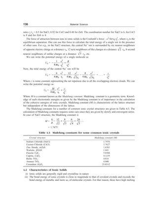
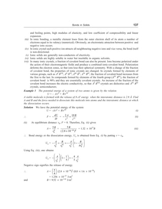
![Bonds in Solids 139
The structure of KCl is identical to that of NaCl. The compressibility is reciprocal to the bulk modulus, and
hence
1
K
=
0
2
2
0
1
18 R R
d U
NR dR =
æ ö
ç ÷
è ø
(iii)
From Eq. (i), we have
0
2
2
R R
d U
dR =
= 3 2
0 0 0
( 1)
2
4 n
n n NB
NMq
R R
pe
2
+
+
- +
=
3
0 0
2
( 1)
4
NMq
n
R
pe
2
- (Using Eq. (ii))
Hence from Eq. (3.46), we have
n = 1 +
4
0
0
2
18 ( 4 )
R
KMq
pe
= 1 +
10 4
11 19 2 9
18 (3.147 10 )
5.747 10 1.748 (1.6 10 ) 9 10
-
- -
´ ´
´ ´ ´ ´ ´ ´
= 1 + 7.63 = 8.63
Example 3 The force of attraction between ions of Na and Cl is 3.02 ´ 10–9
N when the two ions just
touch each other. Given: ionic radius of Na+
ion is 0.95 Å, e = 1.6 ´ 10–19
C, e0 = 8.854 ´ 10–12
C2
/N – m2
. Find the radius of Cl–
ion. [M. Sc. (MS), B.E.]
Solution We have F1 = –
2
1 2
0 2
4
Z Z e
r
pe
(force of attraction)
F1 = 3.02 ´ 10–9
N =
2 19 2
12 2
( 1) ( 1) (1.6) (10 )
4 8.854 10 r
p
-
-
+ - ´
´ ´
Z1 = +1 for Na+
26
2
0.023
10 N
r
-
= ´ Z2 = –1 for Cl–
r2
=
26
9
0.023 10
3.02 10
-
-
´
´
= 0.0076 ´ 10–17
e = 1.6 ´ 10–19
C
e0 = 8.854 ´ 10–12
r = 0.276 ´ 10–9
m = +
Na
Cl
r r -
+
Cl
r - = 2.76 ´ 10–10
– 0.95 ´ 10–10
= 1.81 ´ 10–10
m
= 1.81 Å
Example 4 The ionic radii of Mg++
and S––
respectively are 0.65 Å and 1.84 Å. Calculate the force of
attraction between these ions. Given: e = 1.6 ´ 10–19
C, e0 = 8.854 ´ 10–12
C2
/N-m2
[AMIE]
Solution Force of attraction Z1 = +2 for Mg++
F1 =
2
1 2
2
0
4
Z Z e
r
pe
Z2 = –2 for S – –](https://image.slidesharecdn.com/s-230301071329-4f25d7e9/85/S-L-_Kakani-_Material_Science_-New_Age_Pub-_2006-BookSee-org-pdf-156-320.jpg)
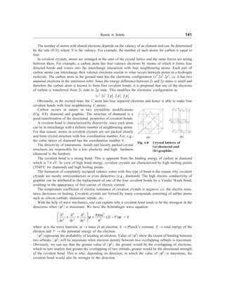
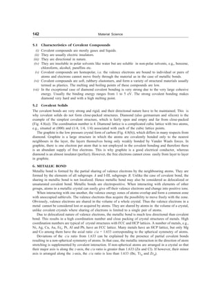
![Bonds in Solids 143
The formation of crystal structures with a BCC lattice is also explained by partial covalent bonds and
non-spherical symmetry of atoms. In these structures, atoms are not packed closely. Crystal structures with
a BCC lattice are typical of Fea, Cr, Mo, W, V, Ta, Tib, Nb, Zrb, and some other metals.
Many metals and some non-metals are polymorphous, i.e., may have different types of crystal structures
in the solid state depending on temperature. Such crystal structures are called allotropic forms, or modi-
fications. They are usually designated by Greek letters a, b, g, d, and so on, with ‘a’ denoting the form
existing at the lowest temperature.
The stability of allotropic modifications at definite temperatures and pressures is determined by the
thermodynamic potential (free energy)
G = H – TS (5)
The modification having a lower algebraic value of thermodynamic potential is more stable at a given
temperature, which can be achieved either by decreasing the enthalpy H or increasing the entropy S.
T
T1
Fig. 4.9 Variations of the
thermodynamic
potentials of two
modifications of
a metal during
heating.
G
BCC
HCP
In metallic crystals, closed-packed structures: HCP (C = 12) and FCC (C
= 12) [Fig. 4.9] have a lower enthalpy and thus are stable at low tempera-
tures (upto T1). The ‘looser’ BCC strucutre (C = 8) has a higher entropy and
therefore is stable at elevated temperatures. This explains the stability of
BCC structures at elevated temperatures in many metals: Ti, Zr, Fe, U. The
stability of the BCC lattice of iron at low temperatures is attributed to an
increase of the electronic component of entropy.
The stability of allotropic modifications may change due to changes in
the type of bond. For example, the tin modification with diamond type
lattice Sna, is stable at low temperatures owing to the high energy of cova-
lent bond, and therefore, low enthalpy. On heating, it changes to the Snb
modification which has a weaker metallic bond.
Around 30 metals, e.g. Titanium, Zirconium, Tin , Uranium, Iron, Cobalt,
etc. exhibit the phenomenon of temperature polymorphism. A high-tempera-
ture modification can be retained in a metal for a long time at 20-25°C by fast cooling, since the diffusion
mobility of atoms at such temperatures is low and cannot cause rearrangement of the lattice.
Besides, some polymorphous transformations occur under the effect of pressure and temperature. For
example, the graphite modification of carbon recrystallizes to diamond when heated to 2000°C under a
pressure of about 1010
Pa. Under very high pressures, iron has a low-temperature modification with HCP
lattice.
An increase of pressure at low temperatures can change less closely packed modifications into close-
packed structures. As has been observed for Ge, Si and Sna, application of a high pressure can change their
covalent crystals with diamond type lattice (C = 4) into metallic crystals with a tetragonal body centered
lattice (C = 8).
The entropy of metallic bond is somewhat lower than that of covalent bond, because of which most
metals have lower melting and boiling points and lower elastic moduli, but higher temperature coefficients
of linear expansion, compared to covalent crystals.
In most cases, an increase of bond energy increases the melting point,elastic modules, an activation
energy of self diffusion, but, on the contrary, decreases the coefficient of linear expansion a. These
regularities have been observed experimentally and have a number of exceptions. In particular, the elastic
modulus of beryllium is anomalously high, because of which beryllium alloys have an elevated stiffness.
Ti and Zr exhibit too low values of elastic moduli and activation energy of self diffusion. The latter explains
their low heat resistance.
By virtue of non-directivity of metallic bonds and close-packed structures, metallic crystals are more
plastic and less hard than covalent crystals. Their high electric conductivity is due to the presence of free
sublevels in valence energy zone.](https://image.slidesharecdn.com/s-230301071329-4f25d7e9/85/S-L-_Kakani-_Material_Science_-New_Age_Pub-_2006-BookSee-org-pdf-160-320.jpg)
![144 Material Science
The temperature coefficient of electric resistance of metallic crystals is positive, i.e., the electric resis-
tance increases on heating.
The metallic bond is weaker than ionic or covalent bond. The binding energy ranges from 1 to 5 eV per
bond.
Quantum mechanically, it can be shown that the wave functions of valence electrons in metals are so
spread out that these electrons can no longer belong to any one nucleus in the solid but are a property of
the solid as a whole. This delocalization of the valence electrons leads to a decrease in both potential and
kinetic energy which is responsible for metallic bonding.
6.1 Characteristics of Metallic Crystals
(i) Metallic compounds are crystalline in nature due to the symmetrical arrangements of the positive ions
in a space lattice .
(ii) Metallic compounds are good conductors of heat and electricity. They have high electrical conduc-
tivity and higher thermal conductivity.
(iii) Metallic bonds being weak, metals have a melting point moderate to high, i.e., the melting points of
metallic crystals are lower than those of electrovalent crystals.
(iv) Metals are opaque to light, because the free electrons in a metal absorb light energy.
(v) Metallic crystals have good lusture and high reflectivity.
7. COMPARISON OF IONIC, COVALENT AND METALLIC BONDS
(i) Ionic and Covalent Bonds: Ionic compounds are crystalline in nature and have high hardness. They are
non-directional and rigid. They have high metting and boiling points. They are poor conductors and exist
in solid form only. They are soluble in water and polar solvents like ammonia but insoluble in organic
solvents.
The ionic character can be calculated from the following relation
% ionic character = [1 –exp{(–1/4) (XA – XB)2
}] ´ 100
where XA and XB are electronegativities of elements A and B respectively, joining the ionic-covalent bond.
Obviously, the ionic character of the bond increases if the electronegativity between the joining atoms
increases. This type of mixed bond is obtained in several semiconducting material is, e.g. Ga As and ZnS.
In ZnS, Zn belongs to II B group and S belongs to VI A group has higher ionic character than Ga As in
which Ga and As respectively belong to III A and V A.
The electronegativities are: Ga – 1.8, As – 2.2
Zn – 1.7, S – 2.4
% Ionic character of Ga As
= {1 – exp[–1/4 (1.8 – 2.2)2
]} ´ 100
= 3.92 %
% Ionic character of ZnS
= {1 – exp [–1/4 (1.7 – 2.4)2
]} ´ 100
= 11.53%
Covalent compounds are rubbery in nature and covalent bonds can be observed in gases, liquids and
many solids. They have low melting and boiling points. With the exception of diamond and graphite,
compounds of covalent bonded materials are usually soft, easily fusible and electrically insulators. They
have open structures and covalent bonds are directional.
(ii) Ionic and Metallic Bonds: Ionic bonds result from the mutual attraction of positive and negative ions.
Ionic compounds have low thermal and electrical conductivity but have fairly high melting points. Ionic
bonds are stronger than metallic bonds. Ionic bond itself is non-directional.
In ionic bonding, a metallic element loses, from the outer electronic shell of its atom, a number of
electrons equal to its valency (numerical). These lost electrons are transferred to the outer electronic shells
of non-metallic atoms with which the metal is combining. In this way, a complete octet of electrons is left
behind in metallic particle and completed in the non-metallic particle, finally both gets stable outer shells.](https://image.slidesharecdn.com/s-230301071329-4f25d7e9/85/S-L-_Kakani-_Material_Science_-New_Age_Pub-_2006-BookSee-org-pdf-161-320.jpg)
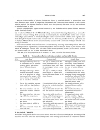
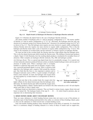
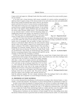
![150 Material Science
the strength of ionic bonds increases with valency. We can easily understand why the melting point of
magnesium oxide is higher as compared to sodium chloride.
One can easily determine the strength of materials and their crystal structure by knowing the bond
strength.
Ionically or covalently bonded materials are non-conductors since their electrons are bound tightly in the
bonds. We can understand that metals are excellent conductors because of the fluctuation of the electron
cloud on application of a potential difference.
Due to shifting of electrons, metals possess ductility. Since the impinging radiant energy is easily
absorbed by valence electrons, metallic bonded materials are opaque and lustrous.
11. PERIODIC TABLE AND CHEMICAL BONDING: ELECTRONEGATIVITY
We have stated earlier that the degree to which an atom can attract electrons to itself, is termed its
electronegativity. In general, it is observed that electronegativity increases steadily across the periodic table
Group I to Group VII. Moreover, electronegativity varies within a group, decreasing with increasing atomic
number, except in the case of transition metals. Two atoms of similar electronegativity, form either a
metallic or covalent bond, depending upon whether they can release or accept electrons. When their
electronegativity is different, the bond is partially ionic and the ionic character increases with the difference
in electronegativity. In general, electronegativity decreases with increase in atomic number, except in case
of transition elements.
We must note that in any one row of the periodic table, (from right to left), the metallic character of the
bond increases and covalent character decreases, whereas in any one column (from top to bottom), the
metallic character increases or the covalent character decreases. From periodic table, we can see that Li,
Na, K, Rb, Ls and Fr are metals with increasing metallic character, whereas at the other end, F, Cl, Br and
I form covalent bonds of decreasing strength. Cs and Fr (at the bottom left of the periodic table) are more
metallic than others and their ionization potentials is the lowest. F and Cl (at the top right-hand corner of
the periodic table) are very non-metallic and exhibit the greatest electron affinity.
The bond between atoms of inert elements, between molecules of group VII, and VI and V, between
molecules of unlike atoms is a weak secondary one.
We find that the transition metals have a partial covalent character and hence their melting points are
high. Fe (1535°C), Ni (1453°C), Co (1495°C), V (1900°C), Nb (2415°C), Ta (2996°C), Mo (2610°C), Zr
(1852°C), Ti (1668°C) and W (3410°C) are common engineering metals from the transition series, the
melting point of each of these elements is shown within parenthesis.
Example 5 The outermost electron which can easily be removed from Na atom requires +5.14 eV of
energy. When this electron is transferred to a vacant position on a distant chlorine atom, it gives back
–4.02 eV of energy. How much net energy is spent in the said process? [AMIE, B.Sc. (Hons)]
Solution Net spent energy = +5.14 – 4.02 = 1.12 eV.
Example 6 The enthalpy of fusion of ice is 6.02 kJ/mol. Estimate the fraction of hydrogen bonds that are
broken when ice melts? (Given: Hydrogen bond energy = 20.5 kJ/mol) [B.E.]
Solution There are two moles of hydrogen bonds per mole of H2O in ice. Assuming that all the heat
absorbed during melting goes into breaking the bonds, the fraction of bonds broken =
6.02
20.5 2
´
= 0.15.
We must note that bonds are continuously broken and remade in a liquid, and hence the above value
should be considered as time-averaged value.
Example 7 The enthalpy of atomization of diamond is 713 kJ/mol. The bond energy of the diamond
reported is 347 kJ/mol. Explain the difference between the two. [M.Sc. (M.S.)]](https://image.slidesharecdn.com/s-230301071329-4f25d7e9/85/S-L-_Kakani-_Material_Science_-New_Age_Pub-_2006-BookSee-org-pdf-167-320.jpg)
![Bonds in Solids 151
Solution We know that in diamond, each carbon atom forms four discrete bonds. As two atoms are
required to form a bond, and hence the effective number of bonds per atom is 4/2 = 2. Obviously, when
one mole of diamond is converted into carbon atoms in the gaseous state, 2 moles of C-C bonds are broken.
Therefore, the enthalpy of atomization of diamond = 347 ´ 2 = 694 kJ/mol. We can see that this value is
very close to 713 kJ/mol.
SUGGESTED READINGS
1. L. Pauling, The Nature of the Chemical Bond, Cornell Univ. Press, Ithaca, New York (1960).
2. W.L. Masterton and C.N. Hurley, Chemistry, Principles and Reactions, 2nd ed., Harcourt, Fort
Worth, Tx (2000).
3. J.C. Kotz and P. Treichel, Jr., Chemistry and Chemical Reactivity, 4th ed., Saunders, Fort Worth, Tx
(1999).
4. S.L. Kakani and C. Hemrajni, Solid State Physics, 4th ed., SultanChand, New Delhi-2 (2004).
REVIEW QUESTIONS
1. Describe the nature and origin of various forces existing between the atoms of a crystal. Explain the
formation of a stable bond using the potential energy versus interatomic distance curve.
2. List the various types of bonds occurring in a crystal. Discuss any one of them in brief. [AMIE]
3. Explain electron cloud. What is the role of electron cloud in metallic bond? [Diploma]
4. List the different types of bonds occurring in a crystal. Describe the characteristics of metallic bonds.
[AMIE, M.Sc. (M.S.)]
5. Describe the binding of atoms in metals. [Diploma]
6. Distinguish between ionic and metallic bonds in solids. Illustrate with examples. [AMIE]
7. Why are close-packed structures experienced mostly in metals and not in ionic and covalent bonds?
[B.E.]
8. Explain the origin of metallic bonding. How does it differ from ionic bonding? Explain with suitable
examples. [AMIE, Diploma]
9. How are atoms held together in a metallic bond? Explain diagrammatically. [Diploma]
10. What is hydrogen bond? How is it different from a dipole bond? Explain the role of hydrogen bond
during the formation of ice?
11. Derive an expression for the binding energy of an ionic crystal and obtain the expressions for
Madelung constant. Evaluate the Madelung constant for a linear ionic crystal.
12. What are various types of bonding in materials? Explain the different types of bonding and illustrate
them with suitable examples. [AMIE]
13. How do the melting points of the ionic solids vary?
14. Why do inert gases get liquified and solidified at very low temperatures?
15. Define cohesive energy and determine its value for crystals of inert gases.
16. Using the concept of wave mechanics, explain why a covalent bond tends to be the strongest in the
directions when |y2
| is a maximum. [AMIE, BE]
17. Explain why carbon atoms in diamond bond covalently, while lead atoms bond metallically, even
though carbon and lead have four valence electrons each. [AMIE, Diploma]
18. Explain with the help of suitable sketches the various types of bonding in crystals. [AMIE]
19. Describe the ionic bonding and giving example show that the bond energy of ionic bonding decreases
as the size of electrons increases. Explain this behaviour. [M.Sc. (MS)]
20. What is a secondary bond? Explain the concept of dipole bonding. Why are some compounds non-
polar even if they have dipoles?](https://image.slidesharecdn.com/s-230301071329-4f25d7e9/85/S-L-_Kakani-_Material_Science_-New_Age_Pub-_2006-BookSee-org-pdf-168-320.jpg)
![152 Material Science
21. Compare and contrast metallic, covalent and ionic bonds. Give examples. [AMIE]
22. What do you understand by percentage ionic factor of a covalent bonds? [B.Sc. (M.S.)]
23. Explain in which of the ionic and covalent bonds wave characteristics of electrons play important
role? [M.Sc. (M.S.)]
24. Describe the essential features of the following with one example of each category: (a) metallic bond
(b) ionic bond (c) covalent bond [AMIE]
25. Explain briefly: (a) covalent bonding (b) ionic bonding [AMIE]
26. It is observed that CCl4 has no net dipole moment. What inference do you draw about C-Cl bond in
this compound?
27. Describe compounds which show mixed ionic and covalent bonds? [M.Sc. (MS)]
28. The potential energy of a diatomic molecule is given in terms of the interatomic distance r by the
expression: U(r) =
m n
a b
r r
- + , where symbols have usual meaning. Derive an expression for equal
spacing of the atoms and hence obtain the dissociation energy. [B.E.]
29. Explain the origin of Vander Waals forces in molecular crystals. How does the binding due to Vander
Waals forces differ from the binding the valence crystals. [M.Sc. (MS)]
PROBLEMS
1. The potential energy of a system of two atoms is given by
U = –a/r4
+ b/r12
Calculate the amount of energy released when the atoms form a stable bond. Also determine the bond
length. [(4a3
/27b)1/2
, (3b/a)1/8
]
2. Assume the energy of two particles in the field of each other is given by the following function.
U = –a/r + b/r8
where a and b are constants and r is the distance between the centres of the particles. Show that if
particles are pulled apart, the molecules will break as soon as r = (36b/a)1/7
= r0 (4.5)1/7
.
3. The interaction energy of a system of two atoms is given by
U = –A/r6
+ B/r12
The atoms form a stable bond with bond length of 3 Å and bond energy of 1.8 eV. Calculate A and
B. Compute the forces required to break the molecule and the critical interatomic distance for which
it occurs. [4.19 ´ 10–76
J-m6
, 1.53 ´ 10–133
J-m12
, 2.56 ´ 10–9
N, 3.33 ´ 10–10
m]
4. Assume that the energy of two particles in the field of each other is given by U(r) =
8
r r
b
a
- + , where
a, b are constant and r is the distance between the centres of the particles. Show that the two particles
form a stable compound for r = r0 = (8b/a)1/7
and that in the stable configuration, the energy
attraction is 8 times energy of repulsion.
5. Consider a line of alternate positive and negative ions each carrying a charge q. The repulsive
potential energy between the neighbours is given by A/rn
. Show that for a total of 2N ions, the
equilibrium potential energy of the system is
U0 = –(2Nq2
ln 2/r0) (1 – 1/n)
where r0 is the equilibrium interionic distance.
6. The potential energy U of a system of two atoms varies as a function of their distance of separation
r as
U = –A/rn
+ B/rm](https://image.slidesharecdn.com/s-230301071329-4f25d7e9/85/S-L-_Kakani-_Material_Science_-New_Age_Pub-_2006-BookSee-org-pdf-169-320.jpg)
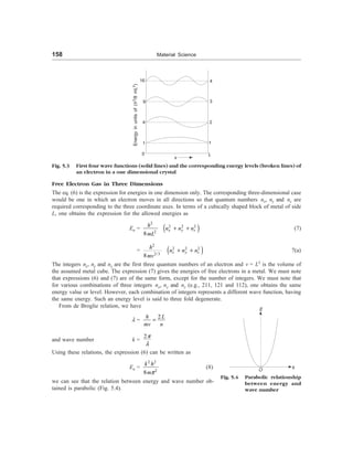
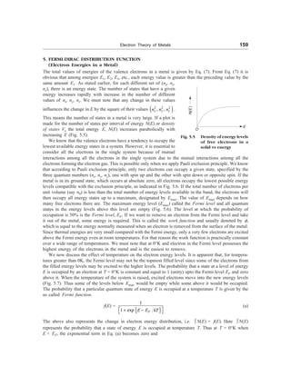
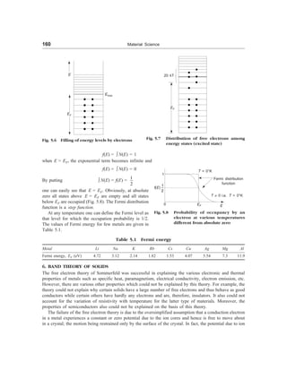

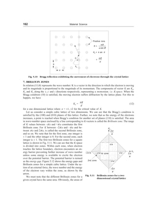
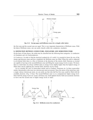
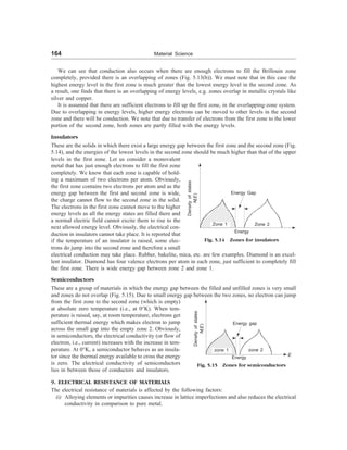
![Electron Theory of Metals 165
In general the resistivity of an alloy is given by the relation
ralloy = rMetal + x rl
where
rmetal = Resistivity of the parent metal,
x = Amount of impurity added in the metal. This is expressed in atomic percent
rl = Resistivity of impure metal
For example, if nickel is added to copper, the resistivity of copper goes up by 1.3 micro-ohm-cm
for each atm. % addition of nickel. One can express this by the following relation
rNi–Cu = rCu + x ´ 1.3 (Micro-ohm-cm)
(ii) The electrical resistance of metallic conductors also increases with increase of temperature.
The relation exhibiting the variation of a metal resistance with temperature is
rt = r20 [1 + a (t – 20)]
where rt ® Resistivity of the metal at t°C, r20 ® resistivity of the metal at 20°C (i.e., at standard
room temperature), and a ® coefficient of temperature resistance.
We must remember that the metals have positive value of temperature coefficient. The higher the
temperature the wider is the thermal vibrations of atoms in the lattice. This causes in atomic spacings
being less regular, i.e., decreasing the mobility of electrons in metals.
(iii) Electrical resistance of a material is affected by the nature of the material, its composition and
condition of its surface.
(iv) Mechanical processes like cold working and increased strain hardening can cause a number of dis-
locations in a material, thereby increasing the electrical resistance.
(v) It is observed that due to age hardening, electron mobility is restricted. This causes the electrical
resistance of the metal increases. It is found that annealing has an opposite effect.
10. ENERGY BANDS
One of the most important reasons for the initial success of the band theory of solids was that it offered
a simple explanation of markedly different electrical behaviour of solids (i.e., conductors, semiconductors
and insulators).
Conductors
A crystalline solid is called a conductor or metal if the uppermost energy band is partly filled [Fig. 5.16(a)]
or the uppermost filled band and the next unoccupied band overlap in energy. Here, the electrons in the
uppermost band find neighbouring vacant states to move in, and thus behave as free particles. When an
electric field is applied, these electrons gain energy from the field and produce an electric current, so that
a metal is a good conductor of electricity. The partially filled band is called the conduction band. The
electrons in the conduction are known as free electrons or conduction electrons. Silver, copper, aluminium,
etc. are few examples of good conductors.
Energy
Conduction
band
Valence
band
(a) Conductors
Energy
Conduction
band
Valence
band
Energy
Conduction
band
Energy gap
Valence
band
(c) Semiconductors
(b) Insulators
Fig. 5.16 Energy band structure (a) metal (b) insulator (c) semiconductor.
Energy gap](https://image.slidesharecdn.com/s-230301071329-4f25d7e9/85/S-L-_Kakani-_Material_Science_-New_Age_Pub-_2006-BookSee-org-pdf-182-320.jpg)
![166 Material Science
Insulators
In some crystalline solids, the forbidden energy gap between the uppermost filled band, called the valence
band, and the lowermost empty band, called the conduction band, is very large [Fig. 5.16(b)]. In such solids
at ordinary temperatures only a few electrons can acquire enough thermal energy to move from the valence
band into the conduction band. Such solids are known as insulators. Since only a few free electrons are
available in the conduction band, an insulator is a bad conductor of electricity. It has been observed that
if the temperature of an insulator is increased, some electrons do jump to the conduction band. Therefore
a small electrical conduction may take place. Most covalent solids, which are composed of atoms having
an even number of valence electrons, are insulators. Rubber, bakelite, mica etc. are good examples of
insulators.
Semiconductors
A material for which the width of the forbidden energy gap between the valence and the conduction band
is relatively small (~1 eV) is referred as semiconductor [Fig. 5.16(c)]. Germanium and Silicon having
forbidden energy gaps of 0.78 and 1.2 eV respectively at 0K are typical semiconductors. As the forbidden
gap is not very wide, some of the valence electrons acquire enough thermal energy to go into the conduction
band. These electrons then become free and can move about under the action of an applied electric field.
The absence of an electron in the valence band is referred to as a hole. The holes also serve as carriers
of electricity. The electrical conductivity of a semiconductor is less than that of a metal but greater than
that of an insulator. The energy gaps of some insulators and semiconductors are given in Table 5.2.
Table 5.2 Energy gaps (eV)
Insulators Energy gap (eV) Semiconductors Energy gap (eV)
Diamond 5.33 Silicon 1.14
Zinc oxide 3.2 Germanium 0.67
Silver chloride 3.2 Tellurium 0.33
Cadmium sulphide 2.42 Indium antimonide 0.23
The electrical conduction in semiconductors which we have described is called instrinsic conductivity.
The conductivity of a semiconductor can also be enhanced by the addition of certain impurities.
11. EQUATION OF MOTION OF AN ELECTRON
According to Drude-Lorentz theory, the motion of electrons is random (when no electric field is applied).
Obviously, the number of electrons in a metal moving from left to right at any time is the same as that
moving from right to left. This shows that no net current flows through the metal. However, if we apply
an electric field across a metal, the electrons move in the positive direction of the field and current is
produced.
Let us consider that an electron within a metal moving in any direction and at any time under the applied
field ‘E’. Let m is the mass of an electron, n is the velocity of the electron and e be the charge on the
electron. The force experienced by an electron due to the applied electric field, E is
F = eE (13)
Due to this force, the electron moves with an average acceleration, d2
x/dt2
(= dv/dt). The force with which
the electron moves,
F = m
dv
dt
(14)
from (13) and (14), we have
m
dv
dt
= eE](https://image.slidesharecdn.com/s-230301071329-4f25d7e9/85/S-L-_Kakani-_Material_Science_-New_Age_Pub-_2006-BookSee-org-pdf-183-320.jpg)
![Electron Theory of Metals 169
n =
Density
Atomic weight Atomic weight
N Nd
´
=
Example 1 Evaluate the temperature at which there is one per cent probability that a state with an
energy 0.5 eV above the Fermi energy will be occupied by an electron. (B.E.]
Solution The probability that a particular quantum state at energy E is filled, is given by
f(E) =
1
1 exp ( )/
F
E E kT
+ -
0.01 =
1
1 x
e
+
E – EF = 0.5 eV
where x =
F
E E
kT
-
f (E) = 1% = 0.01
1 + ex
= 100
ex
= 99
or x = 2.303 log 99
or
0.5
kT
= 2.303 log 99
kT =
0.5
2.303 log 99
´
= 0.109 eV = 0.109 ´ 1.6 ´ 10–19
J
T =
19
23
0.109 1.6 10
0.109
1.38 10
k
-
-
´ ´
=
´
= 1264 K.
Example 2 There are 1019
electrons/m3
, which serves as carriers in a material. The conductivity
of material is 0.01 Ohm–1
/m. Find the drift velocity of these carriers, when 0.17 Volt is applied acorss
0.27 mm distance with the material. Given: e = 1.602 ´ 10–19
C and m = 9.1 ´ 10–31
kg. [AMIE]
Solution E =
V
d
n = 1019
/m3
s = 0.01 Ohm–1
m–1
V = 0.17 Volt
d = 0.27 mm = 0.27 ´ 10–2
m
e = 1.602 ´ 10–19
C
m = 9.1 ´ 10–31
kg
=
3
0.17
0.27 10-
´
= 630 Volt/m
Let v be the drift velocity. The conductivity
s =
nev
E](https://image.slidesharecdn.com/s-230301071329-4f25d7e9/85/S-L-_Kakani-_Material_Science_-New_Age_Pub-_2006-BookSee-org-pdf-186-320.jpg)
![170 Material Science
or 0.01 =
9 19
10 1.602 10 V
630
-
´ ´
= 2.54 ´ 10–3
v
v =
0.01
2.54
´ 10–3
= 3.93 m/s.
Example 3 Find the conductivity of copper at 300 K. The collision time for electron scattering in copper
at 300 K is 2 ´ 10–14
sec. Given that density of copper = 8960 kg/m3
, atomic weight of copper = 63.54
amu and mass of an electron = 9.1 ´ 10–31
kg. [AMIE, Diploma]
Solution We know that 63.54 gms. of copper contains 6.023 ´ 1023
free electrons (i.e., Avogadro’s
number) as the one atom contributes one electron. The volume of 63.54 gm of copper is 8.9 cc. Obviously,
the number of electrons per unit volume (cc),
Temp = 300 K
Time t = 2 ´ 10–14
s
Density of copper = 8960 kg/m3
At. Wt. of copper = 63.54 amu
m = 9.1 ´ 10–31
kg.
n =
23
6.023 10
63.54/8.9
´
= 8.5 ´ 1022
Number of electrons per cubic meter
n = 8.5 ´ 1022
´ 106
= 8.5 ´ 1028
The conductivity,
s =
19 2 28 14
2
31
(1.6 10 ) 8.5 10 2 10
9.1 10
e nt
m
- -
-
´ ´ ´ ´ ´
=
´
= 4.78 ´ 10–7
mho/m
Example 4 The mean free time between the collisions is 10–14
sec. Find the mobility of electrons?
[AMIE]
Solution We have m =
et
m
e = 1.602 ´ 10–19
C
m = 9.1 ´ 10–31
kg
t = 10–14
sec.
=
19 14
31
1.602 10 10
9.1 10
- -
-
´ ´
´
= 1.76 ´ 10–3
m2
/V-s
Example 5 The conductivity of silver is 6.5 ´ 107
per Ohm per m and number of conduction electrons
per m3
is 6 ´ 1028
. Find the mobility of conduction electrons and the drift velocity in an electric field of
1 V/m. Given m = 9.1 ´ 10–31
kg and e = 1.602 ´ 10–19
C. [M.Sc. (M.S.)]
Solution s = nem
or m =
ne
s
s = 6.5 ´ 107
Ohm–1
-m–1
n = 6 ´ 1023
/m3](https://image.slidesharecdn.com/s-230301071329-4f25d7e9/85/S-L-_Kakani-_Material_Science_-New_Age_Pub-_2006-BookSee-org-pdf-187-320.jpg)
![172 Material Science
where n ® velocity of an electron and t ® collision time or mean free time.
For metals, the velocity of an electron corresponds to that of Fermi energy (EF) and is given by the
relation
nF =
2 F
W
m
(28)
where WF ® Fermi energy in Joules (= 1.602 ´ 10–19
times the Fermi energy in electron volts, i.e. 1.602
´ 10–19
EF) and m = 9.1 ´ 10–31
kg.
Example 7 (i) Estimate the maximum velocity of an electron in a metal in which Fermi energy has a
value of 3.75 eV. Given e = 1.602 ´ 10–19
C and m = 9.1 ´10–31
kg. (ii) What will be the mobility of
electrons when the mean free time between the collisions is 10–14
S? [M.Sc.]
Solution WF = 1.602 ´ 10–19
EF = 1.602 ´ 10–19
´ 3.75
= 6 ´ 10–19
J
(i) nF =
19
31
2 2 6 10
9.1 10
F
W
m
-
-
´ ´
=
´
m/s
= 1.76 ´ 106
m/s
(ii) m =
19 14
31
1.602 10 10
9.1 10
et
m
- -
-
´ ´
=
´
= 1.76 ´ 10–3
m2
/V-s
Example 8 The Fermi level for Potassium is 2.1 eV. Estimate the velocity of electrons at the Fermi level.
Given e = 1.6 ´ 10–19
C and m = 9.109 ´ 10–31
kg. [B.E.]
Solution EF = 2.1 eV
e = 1.602 ´ 10–19
C
m = 9.109 ´ 10–31
kg
t = 1014
s
WF = 1.602 ´ 10–19
EF
= 1.602 ´ 10–19
´ 2.1 J
= 3.364 ´ 10–19
J
The velocity of electrons,
nF =
19
31
2 2 3.364 10
9.109 10
F
W
m
-
-
´ ´
=
´
= 0.86 ´ 106
m/s.
Example 9 Estimate the mean free path of free electrons in pure copper at 4 K. The collision time
for photon scattering at 4 K is 10–9
s. The Fermi energy level for copper is 7 eV. Given: e = 1.602 ´
10–19
C and m = 9.109 ´ 10–31
kg.
Solution t = 10–9
s
EF = 7 eV
e = 1.602 ´ 10–19
C
m = 9.109 ´ 10–31
kg
WF = 1.602 ´ 10–19
EF
= 1.602 ´ 10–19
´ 7
= 11.2 ´ 10–9
J](https://image.slidesharecdn.com/s-230301071329-4f25d7e9/85/S-L-_Kakani-_Material_Science_-New_Age_Pub-_2006-BookSee-org-pdf-189-320.jpg)
![Electron Theory of Metals 173
Velocity of electrons,
nF =
19
31
2 2 11.2 10
9.109 10
F
W
m
-
-
´ ´
=
´
m/s
= 1.57 ´ 106
m/s
Mean free path
l = nF t = 1.57 ´ 106
´ 10–9
= 1.57 ´ 10–3
m = 1.57 mm
Example 10 Find the conductivity of copper at 300 K. The collision time (t) for electron scattering
2 ´ 10–14
s at 300 K. Given e = 9.1 ´ 10–31
kg and m = 9.1 ´ 10–31
kg. [B.E.]
Solution The number of electrons per m3
of copper is obtained as
n =
23
6.023 10 8960
0.06354
´ ´
= 8.50 ´ 1023
/m3
We have, conductivity
s =
2
ne
m
t
=
28 19 2 14
31
8.50 10 (1.602 10 ) 2 10
9.1 10
- -
-
´ ´ ´ ´ ´
´
= 4.8 ´ 107
Ohm–1
-m–1
16. THERMOELECTRICITY
This implies direct conversion of heat into electricity. If an electric circuit is made by connecting two
dissimilar metals and the junctions of the two metals are kept at different temperatures, a current flows in
the circuit in a direction depending on the temperature difference be-
tween the two junctions and the nature of metals. This effect is known
as Seeback effect after the name of the discoverer, Seeback. The electric
current is called the thermoelectric current and is the result of an e.m.f.
in the circuit caused by the temperature difference between the junc-
tions. This e.m.f. is termed as thermo e.m.f. The circuit formed by the
two different metals whose junctions are at two different temperatures
is known as thermocouple (Fig. 5.18).
Copper
A
G
Hot
Junction Iron
B
Cold
Junction
Fig. 5.18 Thermocouple
When the two junctions of a couple are T K and the temperature of one junction is raised by a differential
dT, causing a thermo E.M.F. dE in the circuit, the thermoelectric power of the two metals at temperature
T is defined by
P =
T
dE
dT
(29)
The temperature of the hot junction at which the thermo e.m.f. or the thermoelectric current attains its
maximum is called the neutral temperature tn for the given couple. The temperature of the hot junction
where the thermo e.m.f. or the current is zero and changes direction, is termed as the inversion temperature
ti. The inversion temperature is as much above the neutral temperature as the cold junction is below it
tn =
2
c i
t t
+
(30)](https://image.slidesharecdn.com/s-230301071329-4f25d7e9/85/S-L-_Kakani-_Material_Science_-New_Age_Pub-_2006-BookSee-org-pdf-190-320.jpg)
![176 Material Science
REVIEW QUESTIONS
1. Describe the free electron gas model of metals.
2. Write the expression for the Fermi-Dirac distribution function and discuss its behaviour with change
in temperature.
3. Explain the physical basis of classification of solids into conductors, semiconductors and insulators.
[AMIE]
4. What are the effects of electron energy levels in metals? [AMIE]
5. Discuss the factors which affect the electrical resistance of materials. [AMIE]
6. Explain the difference between conductors, semiconductors and insulators. Give two examples of
each category. [AMIE, B.Sc.]
7. Discuss briefly the Zone theory of solids. [AMIE]
8. Draw the energy band diagram of an insulator. [AMIE]
9. Explain the formation of energy bands in solids or on the energy band diagram for metal, semicon-
ductor and insulator. [AMIE]
10. Distinguish between conductors, semiconductors and insulators. [AMIE]
11. Discuss the following:
(a) electron energies in metals
(b) zones in conductors and insulators
12. Compare the salient features of the band theory vis-a-vis the free electron theory. Discuss the suc-
cesses and failures of these theories.
13. State the Bloch theorem and discuss the importance in the band theory.
14. What is thermoelectricity?
15. What are the uses of thermocouples?
16. Why is a Cu-Fe thermocouple not used to measure temperatures above 250°C?
17. What are Brillouin zones? How are they related to the energy levels of an electron in a metal? How
does zone theory explain the conducting or insulating character of a material?
18. What are Brillouin zones? Illustrate your answer by constructing two Brillouin zones for a square
lattice.
PROBLEMS
1. The atomic radius of silver which crystallizes in FCC structure is 1.4. Calculate the Fermi energy of
silver at 0K. [5.7 eV]
2. Show that the wavelength associated with an electron having an energy equal to the Fermi energy is
given by lF = 2(p/3n)1/3
.
3. Estimate the fraction of electrons excited about the Fermi level at room temperature for Na and Cu.
[0.8%, 0.36%]
4. A copper wire has a resistivity of 1.8 ´ 10–8
W-m at 300°K. Assuming copper is very pure, estimate
the resistivity at 700°C and the percentage change in the resistivity from room temperature to 700°C.
[5.84 ´ 10–8
W-m, and 22.4%]
OBJECTIVE QUESTIONS
1. If the mobility of electrons in a metal increases, the resistivity
(1) decreases (2) increases
(3) first decreases and then increases
(4) first increases and then decreases (1)](https://image.slidesharecdn.com/s-230301071329-4f25d7e9/85/S-L-_Kakani-_Material_Science_-New_Age_Pub-_2006-BookSee-org-pdf-193-320.jpg)

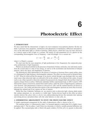
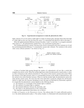
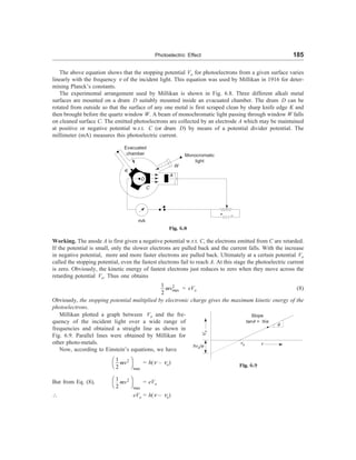
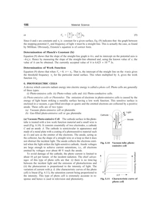
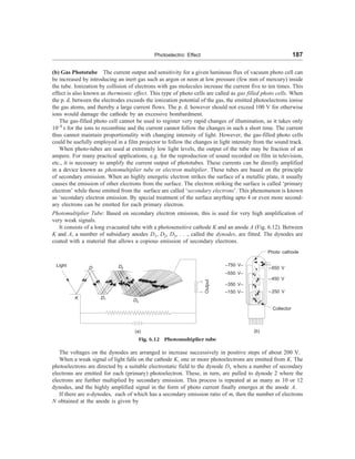
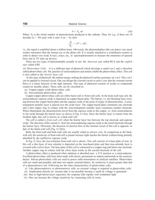
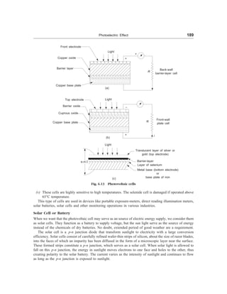
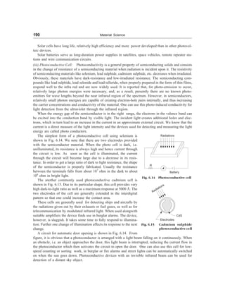
![Photoelectric Effect 191
7. USES OF PHOTOELECTRIC CELLS
The photoelectric cells are widely used in various fields. Some of the important uses are:
(i) In reproduction of sound in motion films
(ii) In television and cathode ray tubes
(iii) In transmission of pictures to distant places (phototelegraphy)
(iv) In photoelectric counters for counting objects
(v) In automatic light switches for switching on and switching off the street light and in other automatic
timing devices
(vi) In burglar alarms to detect thieves and in the fire alarms to indicate the outbreak of fire.
(vii) In determination of temperature of stars
(viii) As illumination-meters in photography, as exposure-meters in photography and as day-light record-
ers in meterology.
(ix) As photoelectric sorter for sorting out objects of different shades.
(x) In photometry
(xi) In fire alarms
(xii) Cell system in hotels
(xiii) Solar batteries
(xiv) Remote sensing in defence work
(xv) Automatic relays
(xvi) Contrast and brightness control in televisions
(xvii) Sorting machines
(xviii) Photostate work or photocopiers
(xix) In the field of communication photocells are used to transmit static images in phototelephones on
infra-red rays without using wires. Photo cells are used in astro compass which finds use in
aeroplanes for autopilot. In the military field photocells are used for signal communication, for
location of invisible rays and in self-aiming projectiles.
Example 1 The wavelength of the photoelectric threshold of tungsten is 2300 Å. Determine the kinetic
energy of electrons ejected from the surface by ultraviolet light of wavelength 1800 Å.
[h = 6.62 ´ 10–34
J-s, c = 3 ´ 108
m/s]
Solution Work function, W = hn0 = hc/l0
=
34 8
10
6.62 10 3 10
2300 10
-
-
´ ´ ´
´
= 0.86 ´ 10–18
J
The energy of the incident radiation is
hn =
34 8
10
6.62 10 3 10
1800 10
l
-
-
´ ´ ´
=
´
hc
J
= 1.10 ´ 10–18
J
Kinetic energy of the ejected electron E is given by
E = hn – W = (1.10 – 0.86) ´ 10–18
J
=
18
19
0.24 10
1.6 10
-
-
´
´
eV = 1.5 eV.
Example 2 The work function of sodium is 2.3 eV. Calculate the threshold frequency and the correspond-
ing wavelength. [AMIE, B.E.]](https://image.slidesharecdn.com/s-230301071329-4f25d7e9/85/S-L-_Kakani-_Material_Science_-New_Age_Pub-_2006-BookSee-org-pdf-208-320.jpg)
![192 Material Science
Solution W = hn0 = 2.3 eV
n0 =
19
34
2.3 1.602 10
6.625 10
-
-
´ ´
=
´
W
h
Hz
Now W = hn0 =
34 8
0 0
6.625 10 3 10
l l
-
´ ´ ´
=
hc
J
(l0 in meters)
=
34 8
19
0
6.625 10 3 10
1.602 10 l
-
-
´ ´ ´
´
eV
(l0 in Å)
=
0
12400
l
eV
The work function of sodium is 2.3 eV
or 2.3 eV =
0
12400
l
l0 =
12400
2.3
= 5390 Å
Example 3 Electrons are emitted with zero velocity from a certain metal surface when it is exposed to
radiations of 6800 Å. Calculate the threshold frequency and work function of the metal.
[AMIE, Diploma]
Solution hn = W +
1
2
mv2
= hn0 +
1
2
mv2
As n = 0,
1
2
mv2
= 0, hn = hn0
or n = n0 =
8
10
3 10
6800 10
l -
´
=
´
c
= 4.416 ´ 1014
Hz
Work function W = hn0 = 6.625 ´ 10–34
´ 4.416 ´ 1014
= 2.918 ´ 10–10
J
Example 4 A blue lamp emit light of a mean wavelength of 4500 Å. The lamp is rated at 150 W and 8%
of energy appears as emitted light. How many photons are emitted by lamp per second?
[AMIE, Diploma]
Solution Light energy emitted/sec = 150 ´
8
100
J = 12 J
n =
l
c
Now hn =
l
c
h
c = 3 ´ 108
m/s
h = 6.625 ´ 10–34
J/s
l = 10–10
m](https://image.slidesharecdn.com/s-230301071329-4f25d7e9/85/S-L-_Kakani-_Material_Science_-New_Age_Pub-_2006-BookSee-org-pdf-209-320.jpg)
![194 Material Science
For barium,
l0 =
4.52
2.5
´ 2746 Å = 4965 Å
SUGGESTED READINGS
1. A. Beiser, Concepts of Modern Physics, 5th ed., McGraw Hill (1996).
2. S.L. Kakani, Modern Physics, Viva Books Pub. New Delhi (In press).
REVIEW QUESTIONS
1. What is photoelectric effect? Write Einstein’s photoelectric equation.
2. What is photoelectric effect? Explain the characteristics of the photoelectric effect.
3. Describe briefly an arrangement for studying the photoelectric phenomenon. Point out the important
features of the experimental results. How did Einstein explain them?
4. Derive Einstein’s photo electric equation and show that the frequency of the incident radiation affects
the photoelectric emission.
5. What is photoelectric effect? Explain the laws of photoelectric emission.
6. How would you explain terms related to photo electric effect?
(i) Threshold frequency (ii) Stopping potential
(iii) Photoelectric work function (iv) Planck’s quantum theory of radiation
(v) Critical wavelength
7. What are the fundamental laws of photoelectric emission? Write Einstein’s photoelectric equation.
8. What is a photo cell? Describe the different types of photoelectric cells? Mention the important
applications of these cells.
9. Describe in brief the emission of photocells and effect of temperature on their emission. [AMIE]
10. What is photoelectric effect? Describe an experiment to verify this law. [AMIE]
11. Describe some of the devices operating on the photoelectric effect. [AMIE]
12. State and explain Einstein’s photoelectric equation. [AMIE]
13. State Einstein’s law for the photoelectric effect. Describe an experiment to verify this law.
[AMIE]
14. State and explain Einstein’s photoelectric equation. [AMIE]
15. Describe Millikan’s experiment for the verification of Einstein’s photoelectric effect.
16. Write short explanatory notes on
(a) Solar batteries (b) Photomultiplier tube
(c) Phototubes (d) Photo sensitive tubes
(e) Photoelectric work function (f) Einstein’s Photoelectric equation
(g) Photovaltaic cell
PROBLEMS
1. Determine the region of the electron spectrum which liberates photo-electrons from potassium. Given
that the work function of potassium is 2.24 eV. [All wavelengths shorter than 5520 Å]
2. Light of wavelength 2000 Å falls on an aluminium surface (work function of aluminum 4.2 eV).
Calculate: (i) the kinetic energy of fastest and slowest emitted photo-electrons (ii) stopping potential
and (iii) cut off wavelength for aluminium. [(i) 2 eV, 0 eV, (ii) 2 V (iii) 3000 Å]](https://image.slidesharecdn.com/s-230301071329-4f25d7e9/85/S-L-_Kakani-_Material_Science_-New_Age_Pub-_2006-BookSee-org-pdf-211-320.jpg)
![Photoelectric Effect 195
3. The work function of a particular emitter is 2 eV and light of wavelength 3000 Å is used to cause
emission. Find the stopping potential and the velocity of the most energetic materials.
[2.14 V, 8.68 ´ 105
m/s]
4. The work function of potassium is 1.9 V. If radiation of wavelength 4.5 ´ 10–7
m be incident on it,
what would be (i) the threshold wavelength (ii) the maximum kinetic energy of ejected electrons and
(iii) the minimum retarding potential? [(i) 6.53 ´ 10–7
m (ii) 1.37 ´ 10–19
J (iii) 0.86 V]
5. The work function for zinc is 3.6 eV. The threshold frequency for the metal is 9 ´ 1014
Hz. Find the
value of Planck’s constant. [h = 6.4 ´ 10–34
J-s]
OBJECTIVE QUESTIONS
1. The work function for aluminium is 4.2 eV. The cut off wavelength for the photoelectric effect for
the surface is
(1) 2955 Å (2) 3100 Å
(3) 4200 Å (4) 1500 Å (1)
2. The work function for aluminium surface is 4.2 eV and that for sodium surface is 2 eV. The two
metals were illuminated with appropriate radiations so as to cause photo-emission. Then
(1) both aluminium and sodium will have threshold frequency
(2) the threshold frequency of aluminium will be more than that of sodium
(3) the threshold frequency of aluminium will be less than that of the sodium. (3)
(4) none of the above
3. X-rays of frequency n are used to irradiate sodium and copper surface in two separate experiments
and the stopping potential determined. Then
(1) the stopping potential is more for copper than sodium
(2) the stopping potential is more for sodium than for copper
(3) the stopping potential is same for sodium and copper
(4) none of the above
4. Light of two different frequencies, whose photons have energies 1 and 2.5 eV respectively succes-
sively illuminate a metal whose work function is 0.5 eV. The ratio of maximum speeds of the emitted
electrons will be
(1) 1 : 1 (2) 1 : 2 (3) 1 : 4 (4) 1 : 5 (2)
5. The work function of a photoelectric material is 3.3 eV. The threshold frequency will be equal to
(1) 4 ´ 1014
Hz (2) 5 ´ 1020
Hz (3) 8 ´ 1010
Hz (4) 8 ´ 1014
Hz (4)
6. Light of wavelength 4000 Å is incident on a metal plate whose work function is 2 eV. The maximum
kinetic energy of the emitted photoelectron would be
(1) 0.5 eV (2) 1.5 eV (3) 20 eV (4) 1.1 eV (4)
7. In photoelectric effect the number of electrons emitted is proportional to
(1) work function of cathode (2) velocity of incident beam
(3) frequency of incident beam (4) intensity of incident beam (4)
8. What is the order of time interval between the falling of radiation on a metallic surface and the
ejection of photoelectron from it?
(1) 10–9
s (2) 10–6
s (3) 10–4
s (4) 10–2
s (1)
9. The threshold wavelength for photoelectric emission from a material is 5200 Å. Photoelectrons will
be emitted when this material is illuminated with monochromatic radiation from a
(1) 50 W infrared lamp (2) 1W infrared lamp
(3) 50 W ultraviolet lamp (4) 1W ultraviolet lamp (3, 4)](https://image.slidesharecdn.com/s-230301071329-4f25d7e9/85/S-L-_Kakani-_Material_Science_-New_Age_Pub-_2006-BookSee-org-pdf-212-320.jpg)
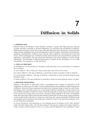
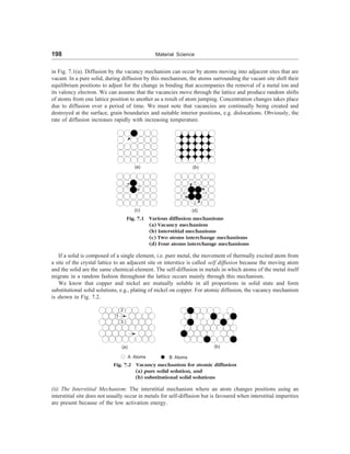
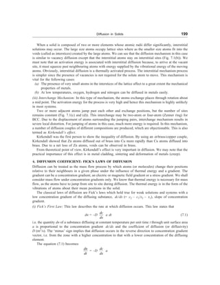
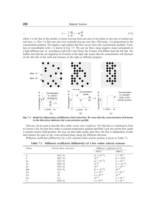
![Diffusion in Solids 201
Parentheses indicate that the phase is metastable
(ii) Fick’s Second Law: This is an extension of Fick’s first law to non steady flow. Fick’s first law allows
the calculation of the instantaneous mass flow rate (flux) past any plane in a solid but provides no
information about the time dependence of the concentration. However, commonly available situations with
engineering materials are non-steady. The concentration of solute atom changes at any point with respect
to time in non-steady diffusion.
If the concentration gradient varies in time and the diffusion coefficient is taken to be independent of
concentration, the diffusion process is described by Fick’s second law which can be derived from the first
law:
dc
dt
=
d dc
D
dx dx
é ù
æ ö
ê ú
è ø
ë û
(7.3)
Equation (7.3) is Fick’s second law for unidirectional flow under non steady conditions. A solution of
Eq. (7.3) is given by
c (x, t) =
A
Dt
exp [–(x2
/4Dt)] (7.3a)
where A is constant. Let us consider the example of self diffusion of radioactive nickel atoms in a non-
radioactive nickel specimen. Equation 7.3(a) indicates that the concentration at x = 0 falls with time as
t–1/2
and as time increases the radioactive atoms penetrate deeper in the metal block [Fig. 7.3(a)]. At time
t1 the concentration of radioactive atoms at x = 0 is c1 = A/(Dt1)1/2
. At a distance x1 = 2 (Dt1)1/2
the
concentration falls to 1/e of c1. At time t2, the concentration at x = 0 is c2 = A/(Dt2)1/2
and this falls to
1/e and x2 = 2 (Dt2)1/2
. These results are in agreement with experiments.
x1 x2
(i) (ii) (iii)
Fig. 7.3 (a) The radioactive sheet of Nickel (shown by shaded section) is kept in contact with a block
of nonradioactive nickel. Radioactive atoms diffuse from the sheet to the bulk metal and
can be detected as a function of time. In figure, the diffusion of atoms is shown (i) for
t = 0, (ii) for t1
, and (iii) t2
with t2
t1
If D is independent of concentration, Eq. (7.3) simplifies to
dc
dt
= D
2
2
d c
dx
(7.4)
Even though D may vary with concentration, solutions to the differential Eq. (7.4) are quite commonly used
for practical problems, because of their relative simplicity. The solution to Eq. (7.4) for unidirectional
diffusion from one medium to another across a common interface is of the general form
c(x, t) = A – B erf (x/2 Dt ) (7.4a)
where A and B are constants to be determined from the initial and boundary conditions of a particular
problem. The diffusion direction x is perpendicular to the common interface. The origin for x is at the
interface. The two media are taken to be semi-infinite, i.e., only one end of each of them, which is the
interface, is defined. The other two ends are at an infinite distance. The initial uniform concentrations of](https://image.slidesharecdn.com/s-230301071329-4f25d7e9/85/S-L-_Kakani-_Material_Science_-New_Age_Pub-_2006-BookSee-org-pdf-218-320.jpg)
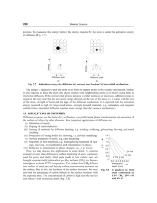
![Diffusion in Solids 207
Modern electronic integrated circuits uses very thin wafers of silicon-diffused with impurities. In doing
so the surface of silicon wafer surface is exposed to vapour of appropriate impurity when wafer surface is
kept at a temperature of about 1100°C in quartz tube furnace. In case if a part of the surface is required
to be kept free from doping, i.e. free from doping, then it can be covered while being treated. We note that
this process is very much similar to the one used for surface hardening of machine parts and the
concentration of impurities from surface reduces almost in the same way as shown in Fig. 7.8.
Example 1 Steel gear, having carbon content of 0.2% is to be gas carburized to achieve carbon content
of 0.96% at the surface and 0.4% at 0.5 mm depth from the surface. If the process is to be carried out
at 927°C, find the time required for carburization. Given, diffusion coefficient of carbon in given steel =
1.28 ´ 10–11
m2
/s. [B.E., M.Sc (M.S.)]
Solution We have
dc
dt
=
2
2
d c
D
dx
(1)
The solution of Eq. (1) can be written as
0
s x
s
c c
c c
-
-
= erf
2
x
Dt
æ ö
ç ÷
è ø
(2)
Substituting the proper values in Eq. (2), we hve
0.9 0.4
0.9 0.2
-
-
= erf
3
12
0.5 10
2 12.8 10 t
-
-
æ ö
´
ç ÷
ç ÷
´
è ø
or 0.7143 = erf
69.88
æ ö
ç ÷
è ø
t
Let z =
69.88
t
erf z = 0.7143 (3)
From table, we find the erf z lies between 0.7112 and 0.7421 for which z lies between 0.75 and 0.80. One
can find the number z by interpolation.
0.7143 0.7112
0.7421 0.7112
-
-
=
0.75
0.80 0.75
-
-
z
or z = 0.755
From (3),
2
2
(69.88)
(0.755)
= t
t = 8566.35 = 142.8 min.
Table 7.1 Error function
z erf z z erf z
0.000 0.0000 0.85 0.7707
0.025 0.0282 0.90 0.7970
0.05 0.0564 0.95 0.8209
0.10 0.1125 1.0 0.8427
x = 0 .5 mm = 0.5 ´ 10–3
m
D = 1.28 ´ 10–11
m2
/s
t = ?
cs ® Surface concentration of diffu-
sion element in the surface = 0.9%
co ® Initial uniform concentration of
the element in the solid = 0.2%
cx ® Concentration of the diffusing
element at a distance x from the
surface = 0.4%
(Contd.)](https://image.slidesharecdn.com/s-230301071329-4f25d7e9/85/S-L-_Kakani-_Material_Science_-New_Age_Pub-_2006-BookSee-org-pdf-224-320.jpg)
![208 Material Science
Table 7.1 Contd.
z erf z z erf z
0.15 0.1680 1.1 0.8802
0.20 0.2227 1.2 0.9103
0.25 0.2763 1.3 0.9340
0.30 0.3268 1.4 0.9523
0.35 0.3794 1.5 0.9661
0.40 0.4284 1.6 0.9763
0.45 0.4755 1.7 0.9838
0.50 0.5205 1.8 0.9891
0.55 0.5633 1.9 0.9928
0.60 0.6039 2.0 0.9953
0.65 0.6420 2.2 0.9981
0.70 0.6778 2.4 0.9993
0.75 0.7112 2.6 0.9998
0.80 0.7421 2.8 0.9999
Example 2 To obtain a p-type semiconductor, boron (an element from third column) is doped in pure
silicon. This doped is carried through a B2O3 vapour phase of partial pressure equal to 1.5 N/m2
. This
atmosphere is equivalent to a surface concentration of 3 ´ 1026
boron atoms per m3
. Show that the time
required to get a boron content of 1023
atoms per m3
at a depth of 2 mm is 3845 s. Given: the doping
temperature = 1100°C and DB in Si at this temperature = 4 ´ 10–17
m2
/s. [B.E., B.Sc. (Hons: M.S.)]
Solution We have
c(x, t) = A – B erf (x /2 Dt )
Using appropriate values, we obtain
erf (x/2 Dt ) = 0.99967
Using table 7.1, we obtain
x/2 Dt = 2.55
t =
2 12
2 17
(2) 10
2 (2.55) 4 10
-
-
´
´ ´ ´
= 3845 sec
Approximate calculations can be made using x = Dt . c1 is negligible compared to c2 and for the diffusion
couple set up, this approximation yields the concentration at x as c(x) = 0.24 c2.
Example 3 The diffusion coefficients of carbon in a-Ti were determined at following temperatures.
Temperature (°C) D (m2
/s)
736 2 ´ 10–13
782 5 ´ 10–13
835 1.3 ´ 10–12
(a) Assuming that Arhenius type rate process equation is valid, find the constant of the equation and
activation energy, and (b) determine the diffusion coefficient at 500°C. [B.E., M.Sc., (M.S.)]
Solution We have
D = D0 exp (–DE/kT) (1)
c1 = 0
cs = 3 ´ 1026
atoms
c(x) = 1023
atoms
x = 2 ´ 10–6
m
D = 4 ´ 10–17
m2
/s](https://image.slidesharecdn.com/s-230301071329-4f25d7e9/85/S-L-_Kakani-_Material_Science_-New_Age_Pub-_2006-BookSee-org-pdf-225-320.jpg)
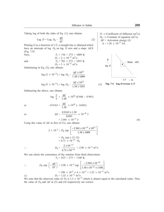
![210 Material Science
Now, using T4 = 500 + 273 = 773 K, one obtains,
D4 = 2.98 ´ 10–4
exp
19
23
2.94 10
1.38 10 773
-
-
é ù
´
-
ê ú
´ ´
ê ú
ë û
´ 1.063 ´ 10–12
= 2.98 ´ 10–4
or Diffusion coefficient at 500°C = 3.17 ´ 10–16
m2
/s
Example 4 The diffusion coefficient for copper in aluminium at 500 and 600°C are 4.8 ´ 10–14
and 5.3
´ 10–3
m2
/s respectively. Determine the approximate time at 500°C that will produce the same diffusion
result (in terms of concentration of copper at some specific point in aluminium) as 10–h
heat treatment at
600°C. [B.E.]
Solution The composition in both diffusion situations will be at the same position, i.e.
x is also a constant. Thus
Dt = constant
Now, D500 t500 = D600 t600
or t500 =
600
500
D
D
t500
=
13 2
14 2
(5.3 10 m /s) (10h )
(4.8 10 m /s)
-
-
´
´
= 110.4 h.
SUGGESTED READINGS
1. P.G. Shewmon, Diffusion in Solids, McGraw Hill, New York (1963).
2. J. Crank and G.S. Park, Diffusion in Polymers, Academic Press, New York (1968).
3. M. Glicksman, Diffusion in Solids, Wiley Interscience, New York (2000).
4. R.J. Borg and G.J. Dienes (Eds.), An Introduction to Solid State Diffusion, Academic Press, San
Diego (1988).
REVIEW QUESTIONS
1. Explain the importance of diffusion in engineering.
2. State and explain Fick’s laws of diffusion. How diffusion coefficient depends upon temperature?
3. Explain the activation energy of diffusion. [A.M.I.E.]
4. Explain the process of diffusion in
(i) ionic crystals and oxides
(ii) Grain boundaries and oxides [B.E.]
5. Explain briefly the following
(i) Diffusion in metals and alloys
(ii) Self-diffusion
(iii) Diffusion coefficients
(iv) Diffusion couple
(v) Diffusion with constant concentration
(vi) Kirkendall effect
(vii) Carburization and decarburization of steel
6. How Fick’s second law can be used to determine D?
7. Explain mechanisms of diffusion.](https://image.slidesharecdn.com/s-230301071329-4f25d7e9/85/S-L-_Kakani-_Material_Science_-New_Age_Pub-_2006-BookSee-org-pdf-227-320.jpg)
![Diffusion in Solids 211
8. How will the diffusivity of NaCl change, when it is doped with (i) KCl and (ii) CaCl2? Explain your
answers. [B.E.]
9. Compare the diffusivities of hydrogen, nitrogen ad nickel in iron at 300 K and explain the difference
between the three values. [B.E., M.Sc, (M.S.)]
PROBLEMS
1. The diffusion rate of A in B was studied at 500°C and 850°C. It was reported that, for the same
diffusion time, the depths of penetration x1 and x2 in the two experiments were in the ratio of 1: 4.
Show that the activation energy of A in B is 57 kJ/mol. [B.E., M.Sc, (M.S.)]
2. An amount Q of a dopant is deposited on the surface of a silicon substrate. During a subsequent
anneal without the dopant in the atmosphere, the concentration c of the dopant as a function of depth
x and time t is given by
c = [Q/ Dt
p ] exp (–x2
/4Dt)
Show that this is solution of Fick’s second law, where D is independent of concentration. [B.E.]
3. The activation barrier for jump is 100 kJ/mol. Calculate the rate at which a vacancy jumps in copper
at 20°C. [1.5 ´ 10–5
/s] [B.E.]
OBJECTIVE QUESTIONS
1. The unit of diffusion coefficient is
(1) m2
s1
(2) m2
s–1
(3) m2
s–2
(4) m2
s2
(2)
2. Substitutional diffusion becomes possible if
(1) the temperature of solid solution is sufficiently high.
(2) the activation energy for vacancy formation is low.
(3) atoms are significantly different in size.
(4) vacancies are present in a substitutional solid solution. (4)
3. The unit of flux J is
(1) moles m–2
s–1
or atoms m–2
s–1
(2) atoms m2
s–1
(3) moles m–3
s–1
(4) moles m–1
s–1
(1)
4. For metal atoms, the most probable mechanism of diffusion is
(1) Vacancy mechanism (2) Interstitial mechanism
(3) Direct interchange mechanism (4) None of the above (1)
5. The dependence of diffusion coefficient on temperature in a certain temperature range is described
by
(1) D = D0 exp (Q/T) (2) D = D0 exp (–Q/RT)
(3) D = D0 exp (–Q2
/RT) (4) D = D0 exp (Q4
/RT) (2)
6. The fastest diffusion coefficient in Fe is
(1) C (2) W (3) Ni (4) H (4)
7. Fick’s first law of diffusion is applicable under
(1) steady state conditions of mass flow
(2) non-steady state conditions
(3) steady as well as non-steady state conditions
(4) none of the above (1)
8. In the presence of impurities and deviations from stoichiometry, the diffusion rate of ions in ionic
crystals
(1) enhances (2) decreases
(3) remains unaffected (4) first decreases and then enhances (1)](https://image.slidesharecdn.com/s-230301071329-4f25d7e9/85/S-L-_Kakani-_Material_Science_-New_Age_Pub-_2006-BookSee-org-pdf-228-320.jpg)
![Mechanical Properties of Materials and Mechanical Tests 215
Elastic region
Plastic region
Load
(Applied)
A Maximum
load
Fracture
C B
Strain
Fig. 8.2 Elastic and plastic regions of materials
(v) Ductility: It is defined as the property of a metal by virtue of which it can be drawn into wires or
elongated before rupture takes place. It is the deformation produced in a material at the breaking point and
measured by the percentage of elongation and the percentage of reduction in area before rupture of test
piece. Its value is expressed as elongation, i.e., percentage elongation is most widely used to measure
ductility. The term percentage elongation is the maximum increase in the length expressed as percentage
of original length. Mathematically, one can express percentage elongation as
Percentage elongation =
Increase in length
Original length
´ 100
= [(lf – lo)/lo] ´ 100
Similarly, the term percentage reduction of cross-sectional area is the maximum decrease in cross-
sectional area. Mathematically, one can express the percentage reduction in cross-sectional area
=
Decrease in crass-sectional area
Original cross-section area
´ 100
= [(Ao – Af)/Ao] ´ 100
In the above relations l and A represent the length and area of cross-section respectively, f and o are
respectively the suffixes to denote final and original values.
Ductility commonly referred to in tensile test, which is strain at fracture. The unit of Ductility is same
as that of strain. As stated above, the valuable information about ductility of a material is obtained from
the form of test curves and by the percentage elongation and percentage reduction in the area of test piece
at the neck. Ductility is a measure of the amount of permanent deformation that has occurred when the
material reaches its breaking point.
We can see that brittle materials, e.g., cast irons show little or no plastic deformation before fracture,
i.e. they are not ductile. A little consideration shows that a metal with a good percentage of elongation or
reduction in cross-sectional area explains its high ductility. Metals with more than 15% elongation are
considered as ductile. Metals with 5 to 15% elongation are considered of intermediate ductility. However,
the metals with less than 5% elongation are considered as brittle ones. Brittle materials such as cast irons
Localised plastic
deformation
Uniform plastic
deformation](https://image.slidesharecdn.com/s-230301071329-4f25d7e9/85/S-L-_Kakani-_Material_Science_-New_Age_Pub-_2006-BookSee-org-pdf-232-320.jpg)
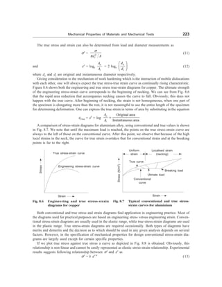
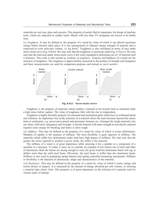
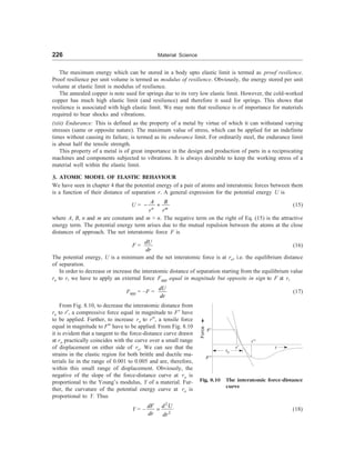
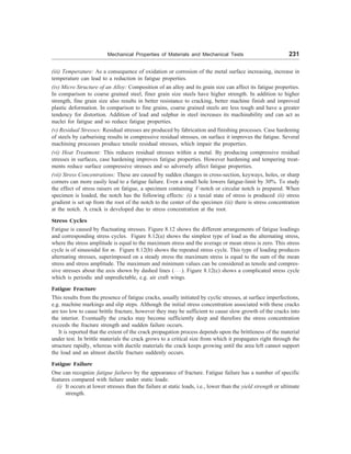
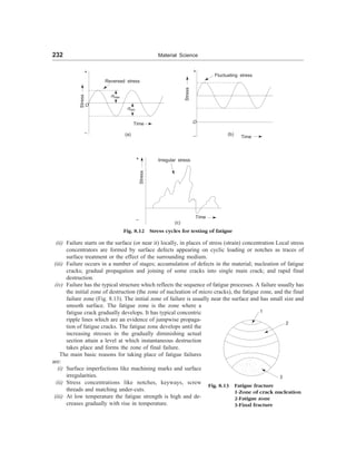
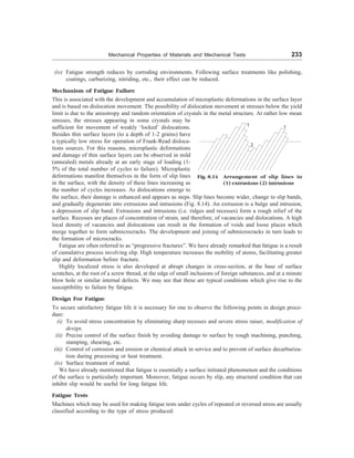
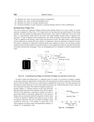
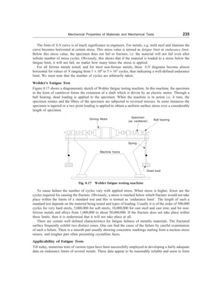
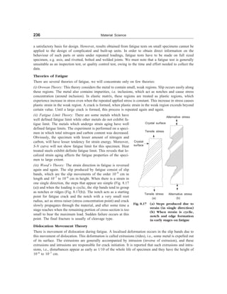
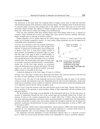
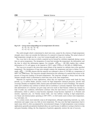
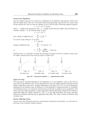
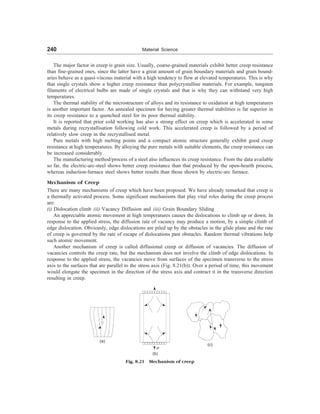
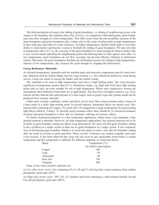
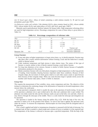
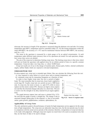
![244 Material Science
To obtain creep resistance at high temperatures, one should observe the following general rules:
(i) Metal with a high melting point be used
(ii) Use FCC metals with low stacking fault energy. For metal with same melting point, the FCC structure
is usually superior to BCC structure in high temperature applications.
(iii) Long range order structure be used. Its behaviour is similar to extended dislocations in FCC lattices.
(iv) Stable precipitants should be used. This will prevent dislocations from excessive gliding by blocking
the glide planes.
(v) Use of those elements be made which precipitate during service time.
(vi) One of the factors affecting the extent of creep is the grain size. Generally coarse grained structure
reveals a better creep resistance than fine grained structure at elevated temperature.
Creep Under the Action of Several Mechanisms
It is very rare that creep deformation takes place only by one mechanism only. Usually creep deformation
takes place when more than one mechanism is operating. Various different mechanisms under certain
conditions control the creep rate. For simplicity purpose, let us assume that creep in a metal is dependent
only on two mechanisms and net creep rate varies with temperature under constant stress. Let the following
two equations represents the creep rate of two simple mechanisms
1
e
= A1 exp [–x1/kT]
2
e
= A2 exp [–x2/kT]
where A1 and A2 are constants at constant stress, e1 and e2 are creep rates and x1 and x2 are activation
energies.
Two creep mechanisms, which are acting simultaneously at one time, can be described as (i) they are
independent of each other and act in parallel and (ii) they act in series, the first mechanism operates first
and second mechanism afterwards. The net strain rate n
e
in the first case is the sum of the individual strain
rates, i.e.
n
e
= 1 2
e e
+
(20)
where e1 and e2 are creep rates respectively for first and second mechanisms. Now, the net creep rate in
the second case is equal to the sum of total strains divided by total time needed for both mechanisms to
function, i.e.
n
e
=
1 2
1 2
t t
e e
+
+
(21)
where e1 and e2 are the respective strains corresponding to respective mechanisms, t1 and t2 are time
intervals between operations of respective mechanisms. Equation (21) clearly reveals that when creep
mechanisms are in series, the one with slower rate or longer delay period controls the creep rate, whereas
Eq. (1) shows that when mechanisms work in parallel the faster rate controls the creep rate.
6. FACTORS AFFECTING MECHANICAL PROPERTIES
The following factors affect the mechanical properties of a
material:
(a) Grain Size This has an important effect on the me-
chanical properties of metals. In comparison to coarse
grained metals, fine grained steels offer better resistance to
cracking, produce fine surface finishes and can be shaped
better. Fine grained steels have higher strength but lower
ductility and therefore, fine grain is specified for structural
applications (Fig. 8.24). Coarse grained steels have higher
hardenability and better forging properties.
Fig. 8.24 Effect of grain size onductility
and tensile strength of metals
Properties
of
metals
Grain diameter
Ductility
Tensile strength](https://image.slidesharecdn.com/s-230301071329-4f25d7e9/85/S-L-_Kakani-_Material_Science_-New_Age_Pub-_2006-BookSee-org-pdf-261-320.jpg)
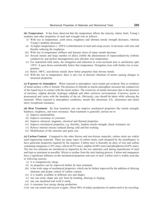
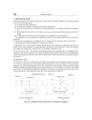
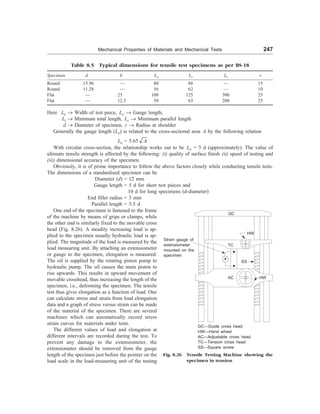
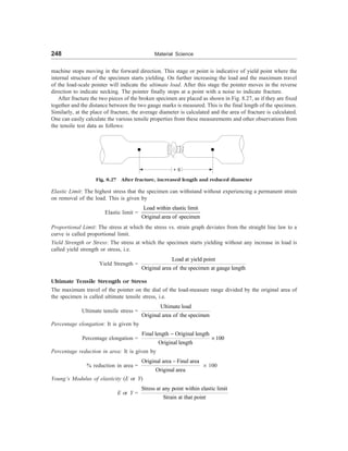
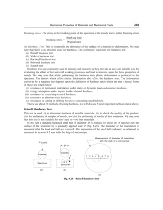
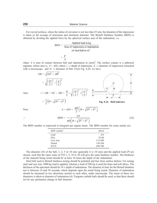
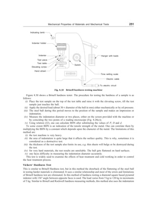
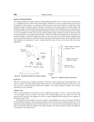
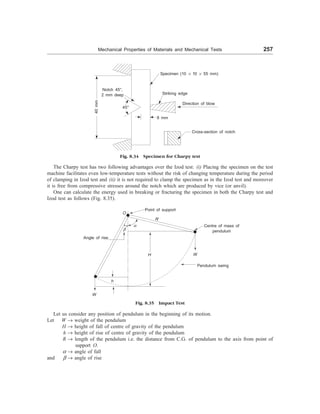
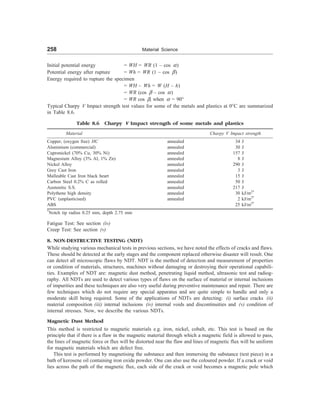
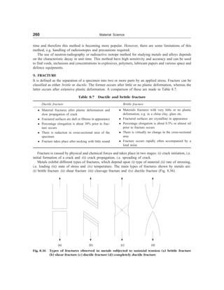
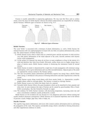
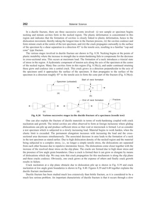
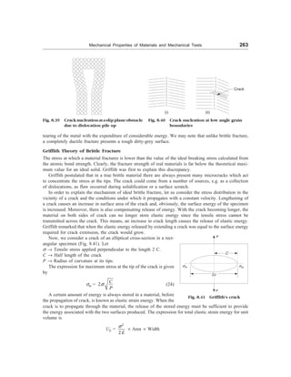
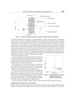
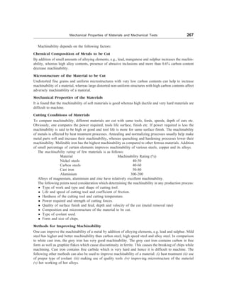
![Mechanical Properties of Materials and Mechanical Tests 269
skill in design to avoid porosity and similar faults. However, this technique lends itself only to relatively
small pieces and to alloys of zinc, aluminium, and magnesium, which have low melting temperatures. This
technique is employed for toys, chasis for radio sets, camperabodies, gears, bearing liners, engine-cylinder-
heads, lead and tin base white metals.
(d) Investment (lost-wax) Casting In case of investment casting, the pattern is made from a wax or
plastic that has a low melting temperature. Around the wax or plastic pattern is poured a fluid slurry, which
sets up to form a solid mould or investment, plaster of paris is usually used. The mould is then heated, such
that the wax or plastic pattern metls and is burned out, leaving behind a mould cavity of desired shape. After
the mould is cooled, the casting is removed by breaking the mould. This technique is an expensive process
for large scale production. This technique is employed when high dimensional accuracy, reproduction of
fine detail, and an excellent finish are desired, e.g., in jewellery and dental crowns and inlays. Also, blades
for gas turbines and jet engine impellers are investment cast. Obviously, this is also suitable for complex
castings.
(f) Continuous Castings At the conclusion of extraction processes, several metals are solidified by
casting into large ingot moulds. Normally, the ingots are subjected to a primary hot-rolling operation, the
product of which is a flat sheet or slab; these are more convenient shapes as starting points for subsequent
secondary metal-forming operations, i.e. forging, extrusion, drawing. One may combine these casting and
rolling steps by a continuous casting (or strand casting) process. Using continuous casting, the refined and
molten metal is cast directly into a continuous strand which may have either a rectangular or circular cross-
section; solidification occurs in a water-cooled die having the desired cross-sectional geometry. In compari-
son to ingot-cast products, the chemical composition and mechanical properties are more uniform through-
out the cross-sections for this type of castings. Moreover, continuous casting is highly automated and more
efficient.
Formability: The ability of metals to be formed into different shapes is termed as formability. Formability
is based on the flowability and ductility of the metal, which, in turn, depends on its crystal structure. The
formability of metals is affected by grain size, hot and cold working alloying elements, and heat treatment
processes, e.g. annealing and normalising.
Low-carbon steel can be easily cold-worked as it has good metal-forming qualities. For metal forming
processes, e.g. rolling, spining, drawing, extrusion, forging, etc., high carbon steel are unsuitable. In order
to prevent the distortion of crystals during cold working, hot working processes are suitable for increasing
the ductility as well as formability of crystals.
We may note that the metal to be deformed during forming process must not crack under the action of
high deforming forces. Such cracks may arise if metal has reached its strain hardening capacity to the full
extent. One can obtain the reliable information on the flow stress from tension or compression test but
unfortunatively only at low strain rates. However, the testing of metals at high strain rate and high tempera-
ture is difficult and lacks testing facilities. For quite some time the single blow test under impact load has
helped to provide indications whether a metal can be hot worked without developing cracks. To assess the
materiability for hot forging and hot piercing, hot twist test has been used. In hot piercing process, solid
cylinders are converted into stainless tubes. In hot twist test the metal cylinder is twisted at high rate and
the torque required to cause given amount of twist is used to calculate the flow stress while number of twists
prior to fracture provides the measure of ductility.
Example 1 The Young’s modulus of a certain material is 180 ´ 103
mega Newton/m2
and its true surface
energy is 1.8 J/m2
. The crack length is 5 mm. Show that its fracture strength is 273 ´ 106
N/m2
. Interpret
your result. [BE, 1999]](https://image.slidesharecdn.com/s-230301071329-4f25d7e9/85/S-L-_Kakani-_Material_Science_-New_Age_Pub-_2006-BookSee-org-pdf-286-320.jpg)
![270 Material Science
Solution The fracture strength is
sf =
2 E
c
g
p
g = 1.8 J/m2
E = 180 ´ 109
N/m2
c =
5
2
´ 10–6
=
9
6
2 1.8 180 10
3.14 5/2 10-
´ ´ ´
´ ´
= 273 ´ 106
Newton/m2
= 273 MN/m2
We note the above calculated strength is approximately ¼ of the actually observed value. The reason
for the difference between the two values is as follows. When the material is deformed plastically and the
crack propagate, then the plastic work is done by the crack. When the crack is plastically deformed, energy
is also consumed. Since we have not taken into account the plastic work required to propagate the crack
and hence the calculated value is lower. One can calculate the amount of plastic work required to propagate
the crack by the equation
sg =
1/2
2 ( )
E p
c
g
p
+
é ù
ê ú
ë û
where sg is actual fracture strength and p is the plastic work required to propagate the crack.
1000 =
9
6
2 180 10 (1.8 )
3.14 2.5 10
p
-
é ù
´ ´ +
ê ú
´ ´
ê ú
ë û
p = 25.32 J/m2
= 12.4 g
which is 12.4 times the surface energy. This shows that the effective surface energy that includes plastic
work is 12.4 times higher than its true surface energy.
Example 2 A tensile test specimen having a diameter of 12.7 mm was loaded upto a load of 76 kN and
its diameter was measured as 12 mm. Compare true stress and strain with engineering stress and strain.
[BE, 2000]
Solution Initial area of cross-section (A0) = 2
0
4 4
d
p p
= (12.7)2
= 126.6 mm2
The area of cross-section after load of 76 kN (A)
=
4
p
d2
=
4
p
(12)2
= 113.04 mm2
Engineering stress (s) =
0
76000
126.6
P
A
= = 600.3 N/mm2
True stress (s¢) =
76000
113.04
P
A
= = 672.33 N/mm2
True strain e¢ = log
0
A
A
= log
126.6
113.04
= 0.113](https://image.slidesharecdn.com/s-230301071329-4f25d7e9/85/S-L-_Kakani-_Material_Science_-New_Age_Pub-_2006-BookSee-org-pdf-287-320.jpg)
![Mechanical Properties of Materials and Mechanical Tests 271
Also e ¢ = log (1 + e)
= 0.113
1 + e = e0.113
= 1.12 e = 0.l2
Example 3 A cast iron bed plate for a pump has a crack length of 100 mm. The Young’s modulus of C.I.
is 210 GN/m2
and the specific surface energy is 10 J/m2
. Show that the fracture strength required is 1.6
´ 108
N/m2
. [BE, 2002]
Solution s =
1/2
2 E
c
g
p
æ ö
ç ÷
è ø
=
1/2
9
6
2 10 210 10
3.14 50 10-
æ ö
´ ´ ´
ç ÷
´ ´
è ø
= (2.67 ´ 1016
)1/2
N/m2
= 1.6 ´ 108
N/m2
Example 4 A piece of copper originally 305 mm long is pulled in tension with a stress of 276 MPa. If
the deformation is entirely elastic, find the resultant elongation? [BE, 2002]
Solution Since the deformation is elastic, strain is dependent on stress,
s = eE (i)
Moreover, the elongation Dl is related to original length l0 as,
e =
0
l
l
D
(ii)
Combining (i) and (ii) and solving for Dl, we have
Dl =
0
l
E
s
=
3
(276 MPa) × (305 mm)
110 10 MPa
´
Example 5 Compute the strain-hardening exponent n in sT = n
T
Ke , for an alloy in which a true stress
of 415 MPa produces a true strain of 0.10. Given K = 1035 MPa. [BE, 1998]
Solution sT = n
T
Ke
Taking log of both sides and solving for n, we have
n =
log log
log
T
t
K
s
e
-
=
log (415 MPa ) log (1035 MPa )
log (0.1)
-
= 0.40
s = 276 Mpa
l0 = 305 mm
e = 110 GPa
= 110 ´ 103
Mpa
= 0.77 mm](https://image.slidesharecdn.com/s-230301071329-4f25d7e9/85/S-L-_Kakani-_Material_Science_-New_Age_Pub-_2006-BookSee-org-pdf-288-320.jpg)
![272 Material Science
SUGGESTED READINGS
1. T.H. Courtney, Mechanical Behaviour of Materials, 2nd
ed., McGraw-Hill (2000).
2. K.G. Budinski and M.K. Budinski, Engineering Materials, Properties and Selection, 7th
ed., Prentice
Hall, NJ (2002).
3. N.E. Dowling, Mechanical Behaviour of Materials, 2nd
Ed., Prentice Hall, Upper Saddle River, NJ
(1998).
REVIEW QUESTIONS
1. Explain the term machinability. Describe the method of improving machinability. [AMIE]
2. Explain weldability and machinability of metal. [AMIE]
3. Differentiate between brittle fracture and ductile fracture. How they are caused. [B. Tech.]
4. Draw a stress-strain diagram for a low carbon steel specimen, indicating the proportionality limit,
elastic limit, yield point and the point of maximum loading and rupture. Explain the above data.
[AMIE, B.E.]
5. Compare and contrast elastic and plastic deformation of materials. [B. Tech.]
6. Define hardness. Discuss its role in characterising mechanical behaviour of materials. [B.E.]
7. What is the effect of stress and temperature on a creep curve? [B.E.]
8. Describe in detail the purpose and procedure for testing of metals for (a) tensile strength and
(b) impact strength. [AMIE]
9. Explain how dislocations produces plastic deformation in materials. [AMIE, B.Tech.]
10. Sketch the conventional and actual stress-strain diagrams and state the significance of each.
[AMIE]
11. Explain the different types of important technological properties of metal. [BE]
12. Explain the phenomenon of creep in metals. How is it controlled? [BE]
13. Sketch a typical creep curve and indicate important stages. Discuss the effect of grain size on creep
strength. [AMIE]
14. What is creep? Draw a typical creep curve and explain the different stages on creep. Elaborate your
answer with reference to steel. [AMIE]
15. Mention the technological properties that control the weldability of metals. [AMIE]
16. Draw S-N curve. Explain different stages occurring in the curve. [BE]
17. When does Hooke’s, law appears to fail? [AMIE]
18. Explain the ‘notch’ sensitivity of metals. [AMIE]
19. What is meant by creep? Explain the different types of creep with the help of creep curve. [BE]
20. With the help of creep curve, discuss three stages of creep. [BE]
21. What is the critical resolved shear-stress [AMIE]
22. Do all metals have endurance limits? Explain. [BE]
23. State the various factors which affect the mechanical properties of materials and state their effects.
[BE]
24. Write factors which contribute to the onset of fatigue failure and those which tend to resist fatigue.
[BE]
25. What are the different methods of determining the hardness of a metal? State their advantages and
disadvantages. [BE]
26. Under what conditions may a ductile material fail in brittle structure? [AMIE]
27. Discuss the examples of ductile and brittle fracture. [AMIE]
28. What is the creep in metallic materials? Why is the knowledge of creep resistance important indus-
trially? [AMIE]
29. Explain the role of fatigue failure behaviour of metals. [AMIE]](https://image.slidesharecdn.com/s-230301071329-4f25d7e9/85/S-L-_Kakani-_Material_Science_-New_Age_Pub-_2006-BookSee-org-pdf-289-320.jpg)
![Mechanical Properties of Materials and Mechanical Tests 273
30. Which element is responsible for the high machinability of free cutting steels? [AMIE]
31. What is meant by the term ‘hardenability’? Discuss, how hardenability of a steel can be estimated.
[AMIE]
32. Describe the methods for minimizing creep of materials at low and high temperatures. [AMIE]
33. Describe tensile testing of metals. What are the data one can get from such a test? [AMIE]
34. Write factors which contribute to the onset of fatigue failure and those which tend to resist fatigue.
AMIE]
35. Why are brittle materials used more often in compression than in tension in structural design?
[BE]
36. Describe in detail the purpose and procedure for testing of metals for (i) tensile strength and impact
strength. [AMIE]
37. Write short notes on the following
(a) Creep of materials (b) Fatigue failure
(c) Ultimate tensile strength (d) Griffith’s crack theory
(e) Ductility (f) Ultimate stress
(g) Fracture (h) Weldability
(i) Elastic strain (j) Endurance limit
(k) Transition temperature (q) Grain-boundary Creep
(m) High temperature creep [AMIE, BE]
38. Differentiate between the following:
(i) Creep and fatigue (ii) Ductility and rigidity
(iii) Ductility and malleability (iv) Ductile and brittle fractures
(v) Kc and Kic of material, and its importance
(vi) Hardness and hardenability
(vii) True stress and Engineering stress
(viii) Elastic limit and proportional limit
(ix) Yield stress and proof stress
(x) Endurance limit and fatigue limit
(xi) Toughness and resilience
(xii) Upper and lower yield points
(xiii) Primary creep, secondary creep and tertiary creep. [AMIE, BE]
39. Discuss the principle of non-destructive testing by the following methods: (a) magnetic dust method
(b) penetrating liquid test and (c) ultrasonic test method. [AMIE, BE]
40. Discuss the effect of dislocation climb and movements of dislocation jogs on creep. [AMIE]
41. What do you understand by creep resisting materials? Give few examples of such materials.
[AMIE]
42. Describe the effect of the following on fatigue
(i) stress concentration on fatigue (ii) size
(iii) change of size of specimen and (iv) surface [AMIE]
43. Discuss briefly the various hardness tests and state the advantages and disadvantages. [AMIE]
44. Discuss the principle of non-destructive testing by the following methods: (i) magnetic dust method
(ii) penetrating liquid test and (iii) ultrasonic test. [AMIE, BE]
45. Name five important mechanical tests which give valuable information about metals and alloys.
[AMIE]
46. What does the impact test signify? Explain with necessary formulations the procedures to be adopted
in an impact test conducted on a pendulum-type impact testing machine. [AMIE, BE]
47. What do you understand by brittle to ductile fracture transition? What is transition temperature?
Describe the factors on which this temperature depends. [AMIE]
48. (a) Explain the Charpy impact test.](https://image.slidesharecdn.com/s-230301071329-4f25d7e9/85/S-L-_Kakani-_Material_Science_-New_Age_Pub-_2006-BookSee-org-pdf-290-320.jpg)
![274 Material Science
(b) Explain the Brinell hardness test for mild steel specimen.
(c) Differentiate between the fracture of mild steel and cast iron specimens in tensile testing.
(d) What factors determine the mechanical properties of materials? Give examples.
(e) How is impact strength measured? Write its SI unit. [AMIE]
49. What are the different non-destructive tests? Explain briefly their fields of application. [AMIE]
50. Explain the Griffith’s theory of metals. Derive the formula for average applied stress at which crack
spreads. [BE]
51. How does corrosion have a deterimental effect on fatigue? How is corrosion fatigue propagated?
What steps would you recommend to minimize it? [AMIE]
PROBLEMS
1. An aluminium rod of 10 mm dia and 300 mm length is subjected to a tensile load of 500 kg. Calculate
the tensile strain, the increase in length and decrease in diameter. The Youngs’s modulus of metal is
0.8 ´ 108
kg/cm2
and Poisson’s ratio is 0.33. [BE]
2. For a brass alloy, the stress at which plastic deformation begins is 345 MPa and the modulus of
elasticity is 103 GPa. (a) What is the maximum load that may be applied to a specimen with a cross-
sectional area of 130 mm2
without plastic deformation? (b) If the original specimen length is 76 mm,
what is the maximum length to which it may be stretched without causing plastic deformation?
[BE], [(a) F = 44,350 N (b) l = 76.25 mm]
3. Consider a cylindrical specimen of some hypothetical metal alloy that has a diameter of 10 mm. A
tensile force of 1500 N produces an elastic reduction in diameter of 6.7 ´ 10–4
mm. Find the elastic
modulus of this alloy, given Poisson’s ratio is 0.35. [BE], [E = 100 GPa]
4. The true strain is eT is defined as
eT = log
i
o
l
l
Show that this may also be represented by
eT = log
o
i
A
A
æ ö
ç ÷
è ø
When specimen volume remain constant during deformation. Which of the two expressions is more
valid during necking? Why?
5. Find the toughness for a metal that experiences both elastic and plastic deformation. Assuming s =
eE for elastic deformation, that the modulus of elasticity is 172 GPa, and the elastic deformation
terminates at a strain of 0.01. For plastic deformation assume the relationship sT = n
T
Ke , values for
K and n are 6900 MPa and 0.30, respectively. Note that plastic deformation occurs between values
of 0.01 and 0.75, at which point fracture occurs. [B.E.], [Toughness = 3.65 ´ 109
J/m3
]
OBJECTIVE QUESTIONS
1. True or False and Justify:
(a) Ductility is measured by the percentage reduction in area before rupture of a test piece.
(b) True stress is lower than engineering stress.
(c) The level of stress at which strain ceases to be wholly elastic is known as elastic limit.
(d) Hardenability is the property of material which enables it to resist abrasion. [BE, AMIE]
2. The measure of ductility is
(1) Percentage elongation (2) modulus of resilience](https://image.slidesharecdn.com/s-230301071329-4f25d7e9/85/S-L-_Kakani-_Material_Science_-New_Age_Pub-_2006-BookSee-org-pdf-291-320.jpg)
![282 Material Science
and nickel to form monel. These two elements are completely soluble in another at all proportions. Brass,
an alloy of copper and zinc, is another example, which forms solid solutions most readily as the atoms of
these two elements have similar sizes and electronic structure unlimited solubility in the solid state can be
observed in copper-gold, and germanium-silicon alloys. Polymorphous metals may possess unlimited solu-
bility within a single modification of the space lattice. For example, Fe= can form a continuous series of
solid solutions with Cr (BCC lattices) and FeC , a continuous series of solid solutions with Ni (FCC lattices).
The formation of solid solutions is always associated with an increase of electric resistance and decrease
of the temperature coefficient of electric resistance. Solid solutions are usually less plastic (except for
copper-based solid solutions) and always harder and stronger than pure metals. Substitutional solid solu-
tions are of two types:
(i) Random substitutional solid solutions and (ii) Ordered substitutional solid solutions.
When there is no order in the substitution of the two metal elements (Fig. 9.1(a)), the chance of one
metal element occupying any particular atomic site in the crystal is equal to the atomic percent of the
element in the alloy. Obviously, in such a situation the concentration of solute atoms can vary considerably
throughout the lattice structure. Such type of the resulting solid solution is called a random or disordered
substitutional solid solution.
(a) (b)
Iron atom
Carbon
atom
(c)
Fig. 9.1 (a) Solid solutions (b) substitutional solid solutions and (c) interstitial solid solution
Many substitutional solid solutions can be in an ordered state at relatively low temperatures, i.e. unlike
atoms of two elements are distributed between the sites of the space lattice not statistically, but in a perfectly
definite order. Such solid solutions are called ordered; the term ‘superstructure’ is also in use. Such
ordering is common at low temperatures because greater thermal agitation tends to destroy the orderly
arrangement. [Fig. 9.1(b)].
The change from a disordered to ordered state takes place at a definite temperature or in a definite
temperature range. The temperature at which a solid solution becomes completely disordered is called the
Kurnakov point (GK). Ordering usually takes place under the conditions when a solid solution is cooled
slowly from the temperature region above GK.
Ordered solid solutions can be found in systems with either substantial or unlimited solubility in the solid
state; in that case complete ordering can occur with concentrations of the solid solution elements correspo-
nding to simple atomic ratios of the components of the type, say AB or AB3. Partial ordering may be obser-
ved in systems with concentration ratios close to the indicated ones. The arrangement of atoms in ordered
solid solutions of two Cu and Au alloys of the corresponding to AuCu3 and AuCu are shown in Fig. 9.2.
The appearance and disappearance of an order in the arrangement of atoms in solid solutions is asso-
ciated with changes in the properties of an alloy.
Ordering increases the electrical conductivity, temperature coefficient of electric resistance, hardness,
and strength, but decreases the ductility of an alloy. In ferromagnetic alloys, it changes magnetic properties;
for instance, the magnetic permeability of perm alloys (magnetic iron-nickel alloys) can drop on ordering
to a small fraction of the original value. Some alloys are paramagnetic in disordered state, but become
ferromagnetic after ordering, such as Heusler (Mn-Cu-Al) alloys.](https://image.slidesharecdn.com/s-230301071329-4f25d7e9/85/S-L-_Kakani-_Material_Science_-New_Age_Pub-_2006-BookSee-org-pdf-299-320.jpg)
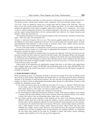
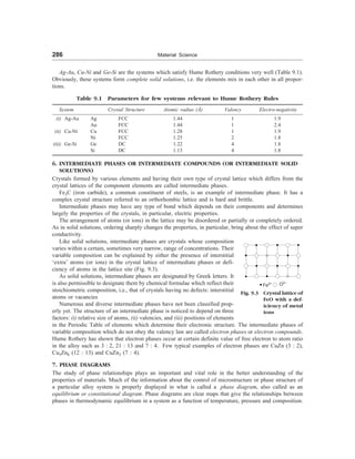
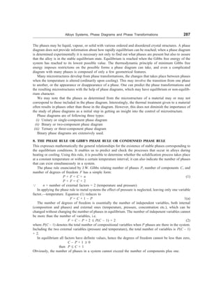
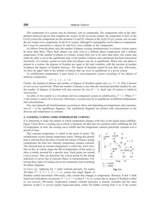
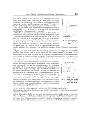
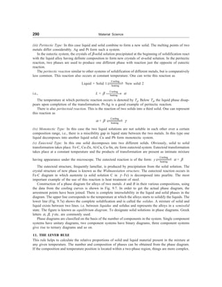
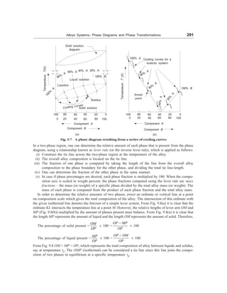
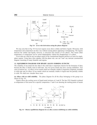
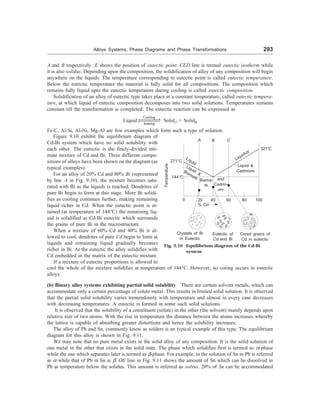
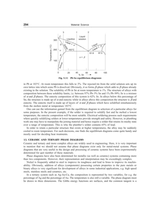
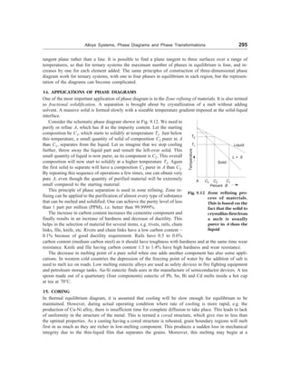
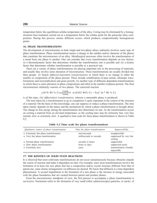
![Alloys Systems, Phase Diagrams and Phase Transformations 297
the new phase, which are capable of growing. It is found that the favourable positions for the formation
of these nuclei are imperfection sites especially grain boundaries. The second stage is growth, in which the
nuclei increase in size. However, during this process, of course, some volume of the parent phase disap-
pears. The transformation reaches completion if growth of these new phase particles is allowed to proceed
until the equilibrium fraction is attained.
(a) Nucleation (Mechanism of Phase Transformation) Let us consider a simple transformation where
a crystal that is in contact with the liquid of the same will grow as liquid freezes. We may consider that
in the beginning, a container is holding both the liquid and solid phases of a pure substance at its melting
point. When heat is removed from the container, the liquid solidifies. We may note that the change from
the liquid to the solid state reflects the tendency of the substance to maintain itself in its most stable, i.e.,
equilibrium state. Since the liquid and the solid can coexist in the equilibrium state at the melting point,
and hence both states are equally stable at this temperature. However, at lower temperature the solid state
is the stable one, while equilibrium at higher temperature demands the liquid state.
At the equilibrium melting point Tm, the free energies of two phases are equal. The Gibbs free energy
DF is considered to be a useful measure of the tendency for a transformation to occur. However, at the
equilibrium point (Tm), there is no tendency for the transformation to occur (enthalpy change), i.e.
DFv = DHv – Tm DSv = 0 [3]
or DSv =
D v
m
H
T
= Change in entropy
Here, we have assumed that DFv and DSv do not vary with temperature. Thus the free energy change
accompanying the solidification at any temperature can be determined as
DFs = DHv – TDSv
= DHv
m
m
T T
T
-
æ ö
ç ÷
è ø
=
D D
H T
Tm
(4)
where DT is the degree of supercooling.
A plot of the variation of free energy during nucleation as a function of particle radius r for different
temperatures is shown in Fig. 9.13.
Surface energy 4Fr 2
+ve
Free
energy
D
F
–ve
Tm
T1
(Critical barrier DF*)
Em
bryos
T2 Supercritical nuclei
Unstable
radius r
r* at T1
E
m
b
r
y
o
s
Volume
free
energy
Tm T1 T2 T3
Stable nuclei
Fig. 9.13 Variation of free energy change ,F during nucleation (solidification), as a function of particle
radius r at different temperatures
T3](https://image.slidesharecdn.com/s-230301071329-4f25d7e9/85/S-L-_Kakani-_Material_Science_-New_Age_Pub-_2006-BookSee-org-pdf-314-320.jpg)
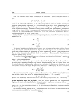
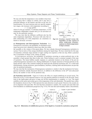
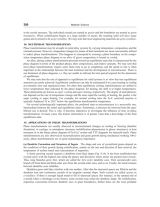
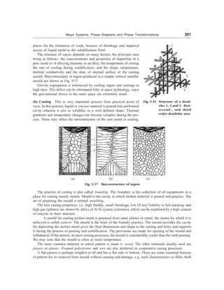
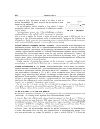
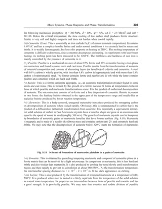
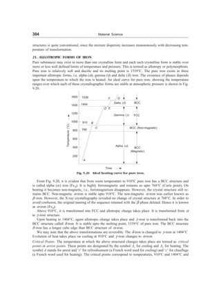
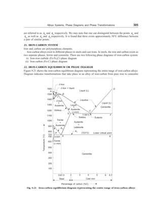
![306 Material Science
(carbon content 6.67%). The carbon percentages is represented on the horizontal axis and the temperature
on the vertical axis. We have also shown the names of the phases existing at temperatures and concentra-
tions determined by the lines (boundaries) of these areas on the equilibrium diagram.
The curve ABCD is called the liquidus. All alloys represented by compositions and temperatures in the
region above ABCD are completely liquids. Point A in the diagram represent the melting point of pure iron
(1539°C). Point D represent the melting point (1539°C) of iron carbide or cementite. With the fall in the
temperature of the liquid along the line ABC, crystals of austenite separate from the liquid. Similarly, in the
same way, crystals of iron carbide (Fe3C) separate from the liquid along the line CD. High temperature
transformation (C – Fe XXV
WXX @ – Fe or FeC
XXV
WXX Fe@) take place at upper left hand portion of phase
diagram (Fig. 9.21). The peritectic reaction HJB represents the formation of austenite, i.e. solid solution of
carbon in gamma iron (C -Fe or FeC ). crystals of @ -iron (Fe@ ) begin to separate from the liquid along the line
AB. We know that a solid solution of carbon in =-iron (Fe= ) at high temperatures is known as @ -iron (Fe@ ).
The complete solidification of iron-carbon alloys proceeds along the line HJECF (Fig. 9.21) called the
solidus. The alloys containing 0.18 to 1.7% carbon represent the solidus HJE and those with carbon
contents ranging from 1.7 to 6.67% become solid along the line ECF at temperature 1130°C. (Fig. 9.21).
At point C in Fig. 9.21 (4.3% carbon), austenite and cementite are simultaneously precipitated from the
alloy to form the eutectic, also called as Lede-burite. The iron-carbon phase diagram (Fig. 9.21) indicates
a peritectic point J, a eutectic point C, and a eutectoid point S. The following reactions takes place at these
points:
(i) During the peritectic reaction (horizontal line HJB at 1401°C)
@-Iron (Fe@) + liquid
Cooling
Heating
XXXXX
V
WXXXX
X Austenite
or FH + LB ® AJ
(ii) At point C the eutectic reaction takes place (4.3%, 1130°C). This can be represented as
Liquid
Cooling
Heating
¾¾¾¾
® Austenite + Cementite (Lede-burite eutectic mixture)
or LC ® [AE + Cem]
(c) At point S (723°C), the eutectoid transformation can be expressed as
Solid
Cooling
Heating
¾¾¾¾
® Ferrite + Cementite or Pearlite (eutectoid mixture)
or AS ® [FP + Cem]
The eutectoid mixture of ferrite and cementite is called pearlite.
The eutectoid (pearlite with 0.8% carbon) and eutectic (ledeburite with 4.3% carbon) are considered as
independent structural constituents which can influence markedly the properties of alloys. Most often
pearlite has a lamellar structure and rather high strength properties.
23. MODIFIED IRON-CARBON PHASE DIAGRAM
In phase diagram of Fig. 9.21, the upper left hand portion, the region ABJN, in which @ -iron may exist is
not very important from practical point of view because temperature near 1401°C are neither used for heat
treatment and not in mechanical working. This is why, it is essential to discuss all the practical aspects of
primary solidification with the modified iron-carbon phase diagram shown in Fig. 9.22.
The study of following two important transformations will clarify the interpretation of phase diagram,
Fig. 9.22:
(i) Primary solidification: i.e, transformation from liquid to solid state.
(ii) Secondary solidification or crystallization: i.e, solid state transformation.
23.1 Primary Solidification
To study these transformations, let us consider the sequence of events when liquid alloys of various carbon](https://image.slidesharecdn.com/s-230301071329-4f25d7e9/85/S-L-_Kakani-_Material_Science_-New_Age_Pub-_2006-BookSee-org-pdf-323-320.jpg)
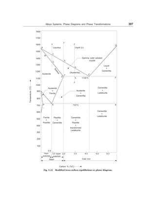
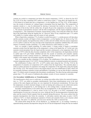
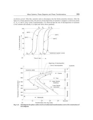
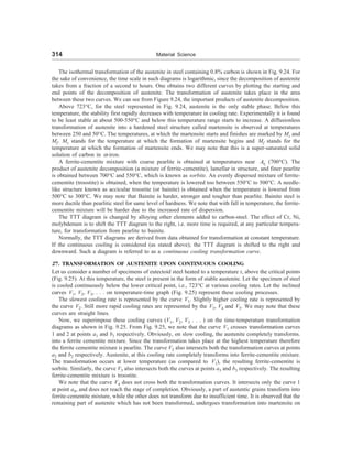
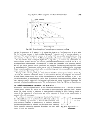
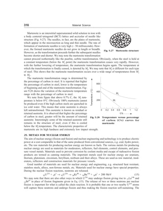
![Alloys Systems, Phase Diagrams and Phase Transformations 317
absorbing capacity of biological protection and fission reaction controlling materials should be high and low
for shell materials. The neutron absorbing capacities and melting temperatures of few materials are given
in Table 9.5.
Table 9.5
Property Cd B Hf Ni Fe Al Zr Mg Be
(i) Effective neutron capaturing 2400 729 115 4.5 2.4 0.23 0.18 0.063 0.01
cross-section area in 10–28
m2
(ii) Melting point temperature (°C) 321 2000 2130 1455 1539 660 1845 651 1280
For the operation of a nuclear power plant is necessary to be able to control the rate of production of
power and also it is necessary to shut the plant whenever required. For this purpose, control rods are used
in nuclear power plants. The fundamental parts of a nuclear power plant or nuclear reactor are: (i) fuel,
(ii) moderator (iii) coolant (iv) control rods (v) pressure vessel (vi) reflector (vii) radiation shield.
Nuclear fuel is made from a fissionable materials like U237
, U235
, Pu239
or Pu241
. Of these U235
is the
only one which is available relatively in plenty. Modern nuclear power plants utilise the uranium fuel as
an oxide (UO2) or a carbide (UC) or a nitride (UN). The main parameters which decide the use of nuclear
fuels in power plants are melting point, specific heat, thermal conductivity, density of metal, and irradiation
stability.
The heat produced in nuclear power plants is intense. Water and gases can be used as heat carriers.
Liquid metals with higher heat conductivity and latent heat and low melting point are employed as heat
carriers. Bismuth and its alloys and sodium are also used. Bismuth is most suitable as it is light and has
low melting point, 217°C. Pb-Bi eutectic alloys (43.5 Pb, 56.5% Bi) is more suitable with lower melting
point of 215°C, less expensive and more fluid although has slightly lower uranium stability and high
absorption capacity for neutrons. Sometimes Lithium is also used.
In order to slow down 2 MeV neutrons produced in the fission process to 0.025 V energies, moderators
are used. Hydrogen, deuterium, beryllium, carbon and oxygen having low atomic mass and small neutron
capture cross-section are used. Boron, cadmium, samarium, hafnium are found suitable for use as a control
material.
Example 1 Find the percentage of proeutectoid ferrite and pearlite in a slowly cooled 0.5% carbon steel.
[Diploma]
Solution Let fulcrum is at 0.5% carbon. We have from lever rule
% Proeutectoid ferrite =
0.80 0.5
0.80 0.0
-
-
´ 100 = 37.5%
% Pearlite ferrite = 100 – 37.5 = 62.5%
Example 2 Determine the degrees of freedom of a system of two components, when the number of phases
is one, two, three, etc. [B.E., M.Sc. (M.S.)
Solution We have F = C – P + N
For C = 2,
one can list the total variables and the degrees of freedom in the following table
No. of Total variables Degrees of freedom
phases P(C – 1) + 2 C – P + 2
1 3 3
2 4 2
3 5 1
4 6 0
In equilibrium, the system cannot have more than four phases.](https://image.slidesharecdn.com/s-230301071329-4f25d7e9/85/S-L-_Kakani-_Material_Science_-New_Age_Pub-_2006-BookSee-org-pdf-334-320.jpg)
![318 Material Science
Example 3 A material of unknown composition at atmospheric pressure (arbitrarily chosen) exhibit four
phases at 987 K. Find the minimum number of components in the system? [BE]
Solution At arbitrarily chosen pressure, one can used the modified form of the phase rule, i.e.
F = C – P + 1
The minimum number of compounds would correspond to minimum degrees of freedom, which is zero.
Thus, taking F = 0, we have
0 = C – 4 + 1
or C = 3
SUGGESTED READINGS
1. P. Gordon, Principles of Phase Diagrams in Material Systems, McGraw Hill, New York (1968).
Reprinted by Krieger Publishing Company, Melbourne, FL (1983)
2. ASM Handbook, Vol. 3, Alloy Phase Diagrams, ASM International, Materials Park, OH (1985).
3. H. Okamoto, Desk Hand book : Phase Diagrams for Binary Alloys, ASM International, Materials
Park, OH (2000).
REVIEW QUESTIONS
1. What is a solid solution? Explain (i) substitutional solid solution and (ii) interstitial solid solution.
Write two examples of each in alloy system. [BE]
2. State Hume Rothery’s rules for the formation of substitutional type of solid solutions. [BE]
3. Carbon when dissolved in iron, forms interstitial solid solution. Explain. [BE]
4. What are three variables that determine the microstructure of an alloy. [Diploma]
5. What thermodynamic condition must be met for a state of equilibrium to exist? [Diploma]
6. What is a solid solution? Discuss the similarities and differences between substitutional and interstitial
solutions.
7. What is solid solution? Give types of solid solution. [AMIE]
8. Draw a schematic TTT curve for a 0.8% plain carbon steel. Label all phase regions. [BE]
9. Draw Fe-C phase diagram. Label all the phases and temperatures properly. Describe the phase
changes during solidification of Fe – 0.45% C alloy. [BE]
10. State and explain ‘Gibb’s phase rule’, defining all terms with examples. [BE]
11. Draw the cooling curves for a binary system forming eutective solution. Explain, how cooling curves
are useful. [BE]
12. Write short notes on the following
(i) Hume-Rothery’s rules (ii) Interstitial compounds
(iii) Gibb’s phase rule (iv) Zone refining
(v) Cooling curves (vi) Various types of solid solutions
(vii) Zone refining (viii) Eutectoid and Peritectic reaction
(ix) Coring (x) Precipitation
(xi) T.T.T. curve [AMIE, BE]
13. Describe the allotropic transformations in iron and explain their importance in practical applications.
[BE]
14. Draw Fe-C phase diagram. Label all the phases and temperatures properly. Describe the phase
changes during solidification of Fe – 0.45% alloy.
[BE]
15. Define critical cooling rate. Give critical cooling rates for different types of carbon steels. [BE]](https://image.slidesharecdn.com/s-230301071329-4f25d7e9/85/S-L-_Kakani-_Material_Science_-New_Age_Pub-_2006-BookSee-org-pdf-335-320.jpg)
![Alloys Systems, Phase Diagrams and Phase Transformations 319
16. What do you understand by critical points and critical range and how are they related to heating and
cooling of steel. Explain their importance in phase transformations. [BE]
17. Why there are tie lines for three phase equilibria but not for two phase equilibrium in a two compo-
nent system? [Diploma]
18. Describe the working of Fe-C diagrams and list the advantages and limitations of these diagrams
when applied to heat treatment. [BE]
19. Explain the working and importance of TTT diagrams. What information is supplied by these dia-
grams? [BE]
20. Describe the process of austenite decomposition of alloyed steels with TTT diagrams. [Diploma]
21. Write short notes on
(i) Martensite (ii) Cementite (iii) Pearlite (iv) Ferrite (v) Pearlite
(vi) Ferrite (vii) Cementite (viii) Bainite (ix) Retained Austenite [Diploma]
PROBLEMS
1. Determine the raction of -phase in an alloy of 80% Sn in the Pb-Sn system at 184°C and 182°C
[BE], [Ans. 0.51, 0.78]
2. Calculate the volume percentage of phase present in an alloy of 16% by weight silicon and 84% by
weight aluminium. Given density of Si = 2.35 gm/cc and density of aluminium = 2.7 gm/cc.
[BE]
3. A Pb-Sn alloy containing 10% Sn is cooled from 200 to 100°C. How much (Wt%) precipitates from
the alloy as a result of the cooling? [Diploma]
4. What is the fraction of proeutectoid cementite in a (i) 1.4% C, (ii) 1.0% C, and (iii) 0.7% C steels?
[Ans. (i) 0.10, (ii) 0.034 and (iii) 0] [Diploma, BE]
5. Derive the degrees of freedom for a system, which has equal number of components and phases.
[Diploma] [Ans. 2]
6. In the Pb-Sn system, calculate the alloy composition at which the fraction of total = is 5/2 times the
fraction of the phase at 182°C. [BE] [Ans. 40.6% Sn]
SHORT QUESTION ANSWERS
1. Why intermetallic compounds are used as bearing materials?
2. Why salt is added into the ice on road in cold countries?
3. Why equilibrium phase diagrams are preferred?
Ans. These are a convenient and concise way of representing the most stable relationships between phases
in alloy systems.
4. What is the use of tie lines and lever rule within two phase regions?
Ans. Tie lines and lever rule are used for computations of phase composition and mass fraction within two
phase regions.
5. What are isomorphous diagrams?
Ans. These are the diagrams for which there is complete solubility in the solid phase. The copper-nickel
system displays this behaviour.
6. What is the significance of phase rule?
Ans. This gives the degrees of freedom that are permissible for a system of a given number of components
and phases in equilibrium.
7. What are the binary phase diagrams?
Ans. These are temperature composition plots, where the pressure variable is omitted.
8. What are the solid state analogue of the eutectic and peritectic reactions?
Ans. Eutectoid and peritectoid reactions are the solid state analogues of eutectic and peritectic reactions
respectively.](https://image.slidesharecdn.com/s-230301071329-4f25d7e9/85/S-L-_Kakani-_Material_Science_-New_Age_Pub-_2006-BookSee-org-pdf-336-320.jpg)
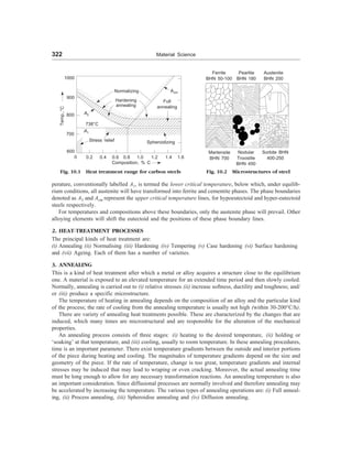
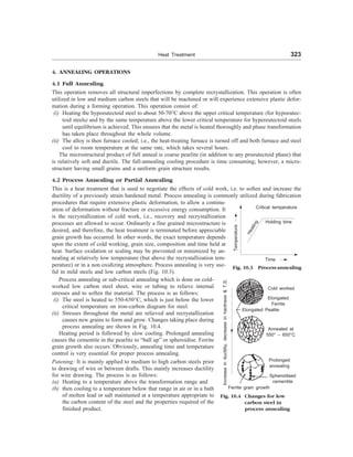
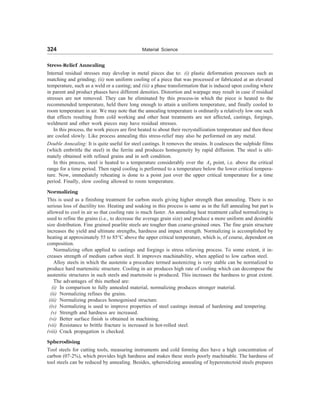
![Heat Treatment 325
their structure to hardening. This type of heat treatment produces carbide in the form of round or globular
(spheroids) instead of plates as in pearlite. This structure gives: good machinability, high ductility and
improvement in formability.
The hardness of a steel is the lowest when the steel structure consists of granular pearlite with inclusions
of rounded-off (spherical) cementitie grains. From this the name ‘spheroidizing’ annealing transpires.
The spheroidizing heat treatment consists of heating the alloy at a temperature just below the eutectoid
phase diagram (line A1 in Fig. 10.1, or at about 700°C] in the a + Fe3C region of the phase diagram. If
the precusor microstructure contains pearlite, spheroidizing times will ordinarily range between 15 and 25
hours. During this heat annealing there is coalescence of the Fe3C to form the spheroid particles.
4.3 Hardening
It is a kind of heat treatment which forms a non-equilibrium structure in an alloy. Non-equilibrium struc-
tures can be produced by heat treatment only in cases when the alloy being treated undergoes certain
transformations in solid solutions, decomposition of a high-temperature solid solution by eutectoid reaction,
etc. To form a non-equilibrium structure in an alloy, it is heated above the temperature of the phase
transformation in the solid state and then cooled (chilled) quickly; fast cooling is essential for preventing
the equilibrium transformation during cooling.
Structural and tool-making alloys are hardened in order to increase their strength. Alloys undergoing a
eutectoid transformation under the equilibrium conditions can be strengthened by hardening quite substan-
tially. Their strength increases either due to the martensitic phase change or due to a reduction of the
temperature of eutectoid reaction; in both cases there forms a fine grained eutectoid mixture. If the hard-
ening procedure has resulted in that the metal at room temperature (20-25°C) has the fixed state of high-
temperature solid solution, the strengthening effect immediately after hardening is insignificant; it will be
pronounced mainly on a repeated low-temperature heating or after holding at 20-25°C.
In alloys possessing special properties, hardening makes it possible to change the structure-sensitive
physical and chemical properties, for instance increases the electric resistance, coercive force or corrosion
resistance.
Hardening capacity and hardenability are important characteristics of steels. Hardening capacity is
defined as the surface hardness of a hardened article and depends mainly on the carbon content of the steel.
We may note that the influence of alloy composition on the ability of a steel alloy to transform to martensite
for a particular quenching treatment is related to a parameter hardenability. Moreover, for every different
steel alloy there is a specific relationship between the mechanical properties and the cooling rate.
‘Hardenability’ is a term that is used to describe the ability of an alloy to be hardened by the formation
of martensite as a result of a given heat treatment. We may note that hardenability is not “hardness”, which
is the resistance to indentation; rather, hardenability is a qualitative measure of the rate at which hardness
drops off with distance into the interior of a specimen as a result of diminished martensite content.
There are two testing methods to measure the hardenability of steels: (i) cylinder series test and
(ii) Jominy end-quench test. The first method gives a single value of hardenability. The value is stated in
terms of percentage of martensite at the centre when quenched in a certain manner. Severity of quench is
an index that quantitatively defines the quenching condition. This index is denoted by H and defined as
H =
Heat transfer coefficient between steel and fluid
Thermal conductivity of steel
When H ® ¥, it represents the severest condition of quench, i.e., surface of steel immediately reaches the
temperature of the quenching medium. Table 10.1 summarizes relative values of H that can be obtained in
various quench media under different condition with value of one for still water as base.](https://image.slidesharecdn.com/s-230301071329-4f25d7e9/85/S-L-_Kakani-_Material_Science_-New_Age_Pub-_2006-BookSee-org-pdf-342-320.jpg)
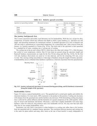
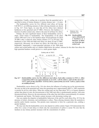
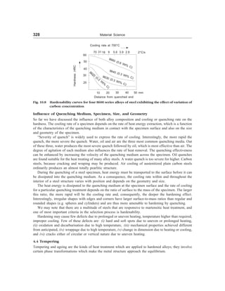
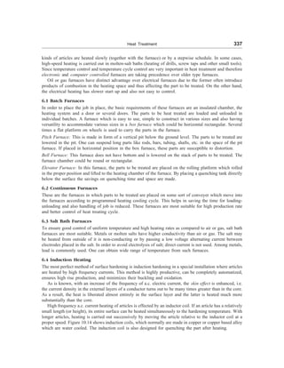
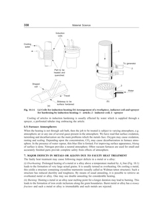
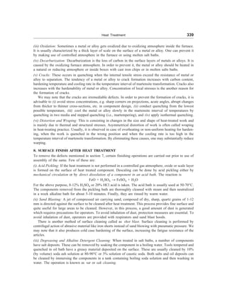
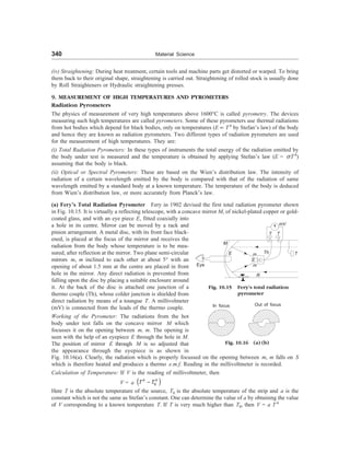
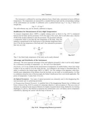
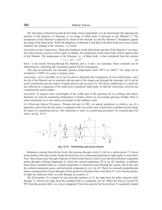
![Heat Treatment 343
till the two patches of light appear equally bright, i.e., light from both the bodies is transmitted equally
through N. The angle through which the Nicol is turned for the purpose is read on a circular scale attached
to it. Let it be q.
Let El be intensity of radiation after filtration through F from the hot body and Sl be the intensity of
radiation of same colour from the standard body, then
E
S
l
l
= tan2
q (4)
Let El ¢ be the intensity of radiation from the second hot body (in place of first body) and q¢, be the angle
of rotation of N, then
E
S
l
l
¢
= tan2
q¢ (5)
From (4) and (5), one obtains
E
E
l
l ¢
=
2
2
tan
tan
q
q ¢
(6)
From Wien’s distribution law, we have
El = A l–5
e–B/lT
and El ¢ = A l–5
e–B/lT¢
(7)
Here A and B are constants and T and T ¢ are temperatures of hot body under test and second body
respectively. Thus, we have
E
E
l
l ¢
=
1 1
B
T
T
el
é ù
-
ê ú
¢
ë û
(8)
From (6) and (8), one obtains
2
2
tan
tan
q
q ¢
=
1 1
B
T
T
el
é ù
-
ê ú
¢
ë û
Taking log of both sides, one obtains
2 (log tan q – log tan q¢) =
1 1
B
T
T
l
é ù
-
ê ú
¢
ë û
(9)
whence, we have a linear relation between log tan q and 1/T, of the form
log tan q = a + b/T (10)
Here a and b are constants and one can obtain them by calibrating the Pyrometer against known tempera-
tures. Knowing a, b and q, one can easily evaluate the temperature of the given hot body.
The normal range of this pyrometer is from 700°C to 1400°C but the range can be raised to 4000°C by
putting absorption glasses in the path of the incident radiation.
Example 1 Determine the grain diameter of an ASTM No. 8. [Diploma]
Solution The grain size specified by the American Society for Testing and Materials (ASTM) is given by
n = 2N–1
where n is number of grains per inch square at a magnification of 100X, and N is ASTM grain size number.
Grain size number 1 to 5 indicates the coarse grain size steel. ASTM number one, is the coarsest grain
which represents one grain per inch square at 100X. ASTM No. 3 represents 4 grains per inch square at
100X and so on. Grain size number 6 and above indicates fine grained steel.
Here N = 8, n = 28–1
= 128](https://image.slidesharecdn.com/s-230301071329-4f25d7e9/85/S-L-_Kakani-_Material_Science_-New_Age_Pub-_2006-BookSee-org-pdf-360-320.jpg)
![344 Material Science
Number of grains/inch2
without magnification = 128 ´ 100 ´ 100
Number of grains/mm2
=
2
128 100 100
(25.4)
´ ´
Average area of each grain =
2
( 25.4)
128 100 100
´ ´
mm2
Average grain diameter =
25.4
100 128
´
= 0.022 mm
The relationship between grain size number and diameter of the grain is given in Table 10.4.
Table 10.4 Relationship between grain size number and actual diameter of the grain
ASTM grain size Grain per inch Actual grain diameter
number, N square at 100 X (inch) (mm)
1 1 0.0100 0.25
2 2 0.0071 0.18
3 4 0.0050 0.125
4 8 0.0035 0.091
5 16 0.0025 0.062
6 32 0.0018 0.044
7 64 0.0012 0.032
8 128 0.0009 0.022
9 256 0.0006 0.016
SUGGESTED READINGS
1. C.R. Brooks, Principles of the Heat Treatment of Plain Carbon and Low Alloy Steels, ASM Inter-
national, Materials Park, OH (1995).
2. D.P. Henkel and A.W. Pense, Structures and Properties of Engineering Materials, 5th Ed., McGraw
Hill, New York (2001).
3. ASM Handbook, Vol. 4, Heat Treating, ASM International, (1991).
REVIEW QUESTIONS
1. What do you understand by heat treatment? Mention the various stages of heat treatment procedure.
2. How is a piece of steel austenitized? Why are time and temperature of austenitizing very important
in heat treatment of steels? [BE]
3. Explain why: (a) Carburising heat treatment is generally on low carbon steels? (b) Alloying elements
in general increase hardenability of steels and (c) Metals undergoing cyclic loading are case hardened.
[Roorkee]
4. What are three steps in an age hardening (heat) treatment? Describe what happens in each step?
[Roorkee]
5. (i) Explain the various purposes of heat treatment. (ii) Describe the flame hardening process and its
application, (iii) Explain the process of annealing. [AMIE]
6. Why must water quenching be used to harden plain carbon steels, while some alloy steels can be
hardened by air cooling? [BE, M.Sc. (M.S.)]](https://image.slidesharecdn.com/s-230301071329-4f25d7e9/85/S-L-_Kakani-_Material_Science_-New_Age_Pub-_2006-BookSee-org-pdf-361-320.jpg)
![Heat Treatment 345
7. Distinguish between hardness and hardenability of a steel. State the factors which affect hardenability.
[AMIE]
8. What factors have to be considered in determining the type of quenching to be used to harden a steel?
[AMIE]
9. Distinguish between full annealing and process annealing. [AMIE]
10. What is meant by the term hardenability? Describe how hardenability of a steel can be estimated.
[AMIE]
11. Explain different types of annealing treatments and their objects. [AMIE]
12. What is the minimum carbon content percentage required in steel so that it may respond to hardening
by heat treatment? [AMIE]
13. Explain the theory of ‘tempering’. What are the effects of tempering on the mechanical properties of
steel. [BHU]
14. (i) Define the term ‘heat treatment’. Why are the steels heat treated? (ii) Discuss the major defects
in steel due to faulty heat treatment. [AMIE]
15. Differentiate between hardness and hardenability. Draw hardness and hardenability curves for steel.
[AMIE]
16. Discuss the use of hardenability curves. [AMIE]
17. (a) Describe the flame hardening process with the aid of a sketch. (b) Describe the main features of
martensite transformation (c) State the objectives of heat treatment of metals. State the process of
tempering. [AMIE]
18. What type of heat treatment is given for die steels? [AMIE]
19. Distinguish between
(a) Hardness and Hardenability
(b) Full annealing and Process Annealing
(c) Martempering and Tempering
(d) Annealing and Tempering
(e) Hardness and Hardening
(f) Solute and Precipitation Hardening [AMIE, BE]
20. Outline the significance of hardenability. How is it measured? Describe some hardening methods.
[AMIE]
21. Define carburising. Describe the various carburising processes. Why are they preferred over each
other? [BE]
22. Outline the principle of high frequency induction hardening. How is induction hardening carried out.
Mention its advantages, disadvantages and applications. [BE]
23. Describe flame hardening and compare it with induction hardening. Describe its merits and demerits
and mention its applications. [BE, B.Sc. (H)]
24. Write short notes on the following:
(i) Age hardening heat treatment (ii) Normalising (iii) Full annealing and process annealing (iv) Case
hardening (v) Annealing (vi) Nitriding (vii) Cyaniding (viii) Spheroidising [AMIE]
PROBLEMS
1. Two specimens of an Fe-3% Silicon-alloy, having grain sizes of ASTM 1 and 8 respectively, yield
at 118 and 207 MNm–2
. Calculate the yield strength of a single crystal of the alloy. [IIT]
2. A cylindrical piece of 8660 steel is to be austenitised and quenched in moderately agitated oil. If the
hardness at the surface of the piece must be at least 50 HRC. Determine the maximum allowable
diameter. [Ans. 95 mm] [BE]](https://image.slidesharecdn.com/s-230301071329-4f25d7e9/85/S-L-_Kakani-_Material_Science_-New_Age_Pub-_2006-BookSee-org-pdf-362-320.jpg)
![Heat Treatment 347
(e) In case of selective heating, time available to change the of steel is short.
(f) Jominy test also gives the hardness at different rates. [Diploma]
2. State whether the following statements are True/False
(a) Oil quenching is required with nitriding.
(b) The size of austenite grains increases with increase in temperature and time of heating.
(c) Tempering temperature below 200°C relieves the hardening stresses.
(d) Age hardening is mainly employed to improve the physical properties of ferrous alloys.
(e) When the steel is heated to its hardening temperature, it becomes pearlitic. [Diploma]
3. Which one of the following is not equilibrium heat treatment
(1) Austenetising (2) Annealing
(3) Normalizing (4) Precipitation (4)
4. Chemical heat treatment involves use of some chemical in conjunction with (heating)
5. Austenitizing is a function of two variables and . (temperature, time)
6. Spheroidising is principally used for steels which are more difficult to form (shape)
(high carbon)
7. The hardenability is not affected by
(1) air (2) chemical composition of steel
(3) critical cooling rate (4) quenching medium and method of quenching
(1)
8. The slowest cooling rate is obtained when steel is quenched in
(1) air (2) brine (3) fused salt (4) mixture of oil and water (1)
9. The fastest cooling rate is achieved when steel is quenched in
(1) air (2) oil (3) water (4) brine (4)
10. Which one of the following is not correct
(1) Martensite has a BCC structure
(2) Austenite has FCC structure
(3) Martensite is a solid solution of carbon in BCC iron
(4) The martensite which is formed during quenching is too brittle (1)
11. Hardenability of steel is assessed by
(1) impact test (2) Jominy end-quench test
(3) hardness test (4) non-destructive test (2)
12. Annealing temperature is
(1) same as normalizing temperature
(2) greater than normalizing temperature
(3) less than normalizing temperature
(4) sometimes greater and sometimes lesser than normalizing temperature (3)
13. Heat treatment that requires heating a part below A1 temperature, i.e. between 550°C and 650° is
called as
(1) hardening (2) normalizing
(3) process annealing (4) full annealing (3)](https://image.slidesharecdn.com/s-230301071329-4f25d7e9/85/S-L-_Kakani-_Material_Science_-New_Age_Pub-_2006-BookSee-org-pdf-364-320.jpg)
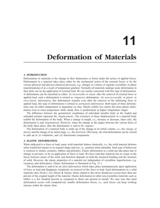
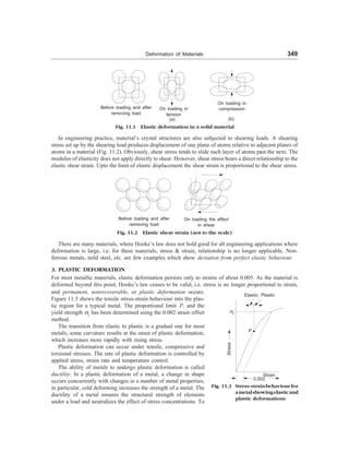
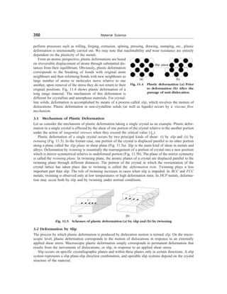
![Deformation of Materials 351
[001]
[101] [ 011]
[010]
[100]
[110]
[101]
[111]
[110]
[011]
[111]
1
2
[111]
[111]
5
4
Deformation by slip can proceed only along the planes and directions having the most dense packing of
atoms (Fig. 11.6). A slip plane together with the direction of slip belonging to that plane forms a slip system.
The slip system depends on the crystal structure of the metal and is such that the atomic distortion that
accompanies the motion of a dislocation is a minimum. The number of slip systems in various metals is
different and depends on the type of crystal lattice. In FCC metals (Cu, Al, Ni, etc.) slip occurs in {111}
planes and 110 directions. The four slip planes in the FCC lattice and three directions of slip in each
of them give 12 equivalent slip systems.
In metals having a BCC lattice, slip develops in {110}, {112} and {123} planes and 111 directions
and the number of slip systems is 48.
In metals with an HCP lattice with c/a ³ 1.63 (Mg, Zn), slip develops in the basal plane which has three
equivalent directions. These metals have a lower ductility than BCC or FCC metals. The number of slip
systems can increase if the critical shear stresses in other planes with less densely packed atoms are
decreased. With an increase of the number of slip systems, the capacity of a metal for plastic deformation
increases. In particular, with c/a 1.63 (as in zirconium and titanium), slip takes place in the basal plane
and the pyramidal and prismatic planes, since the critical shear stresses in these planes have very close
values. For that reason these metals are more ductile than magnesium or zinc in which slip can occur only
in the basal plane. Slip planes, slip directions and number of slip systems observed in various crystal
structures are given in Table 11.1.
Table 11.1 Slip planes, slip directions and slip systems in crystal structures
Crystal structure Slip planes Slip direction Number of slip systems
FCC {111} 110 4 ´ 3 = 12
BCC More common {110} 111 6 ´ 2 = 12
Less common {112}, {321}
ü
ý
þ 12 ´ 1 = 12
24 ´ 1 = 24
NaCl {110} 110 1 ´ 6 = 6
or
6 ´ 1 = 6
HCP More common {0001} Basal Plane
Less common Prismatic 11 2 0
and
ü
ï
ï
ï
ý
ï
ï
ï
þ
closed 3 ´ 1 = 3
Pyramidal planes packed
directions
Al3O2 {0001} 1120 1 ´ 3 = 3
(a) (b) (c)
Fig. 11.6 Slip systems in (a) FCC (b) BCC and (c) HCP lattice metals; planes of the easiest slip are shown
hatched: 1 – (112) plane; 2 – (123) plane; 3 – basal plane; 4 – pyramidal slip plane 5 – prismatic
slip plane.
3](https://image.slidesharecdn.com/s-230301071329-4f25d7e9/85/S-L-_Kakani-_Material_Science_-New_Age_Pub-_2006-BookSee-org-pdf-368-320.jpg)
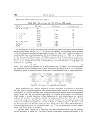
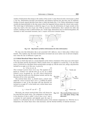
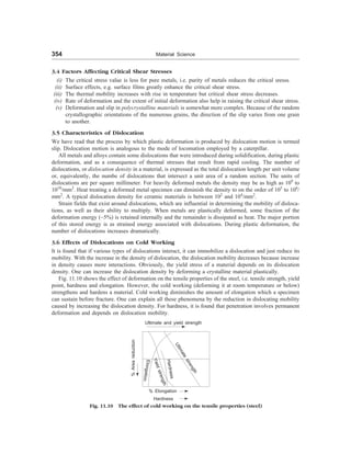
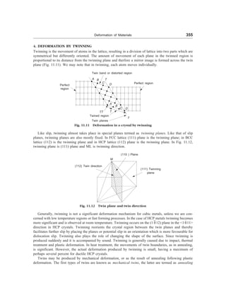
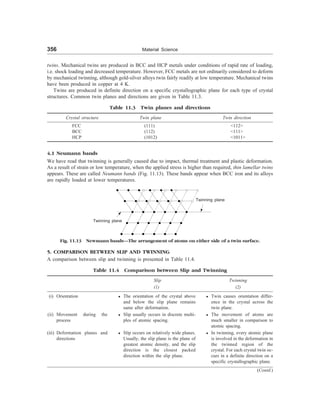
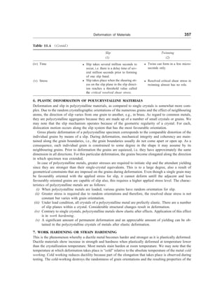
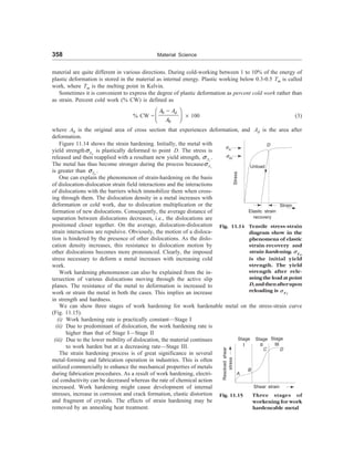
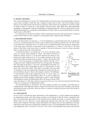
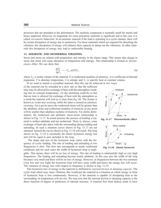
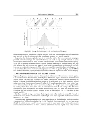
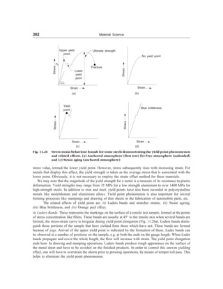
![[S.L._Kakani]_Material_Science_(New_Age_Pub.,_2006(BookSee.org).pdf](https://image.slidesharecdn.com/s-230301071329-4f25d7e9/85/S-L-_Kakani-_Material_Science_-New_Age_Pub-_2006-BookSee-org-pdf-380-320.jpg)
![[S.L._Kakani]_Material_Science_(New_Age_Pub.,_2006(BookSee.org).pdf](https://image.slidesharecdn.com/s-230301071329-4f25d7e9/85/S-L-_Kakani-_Material_Science_-New_Age_Pub-_2006-BookSee-org-pdf-381-320.jpg)
![[S.L._Kakani]_Material_Science_(New_Age_Pub.,_2006(BookSee.org).pdf](https://image.slidesharecdn.com/s-230301071329-4f25d7e9/85/S-L-_Kakani-_Material_Science_-New_Age_Pub-_2006-BookSee-org-pdf-382-320.jpg)
![[S.L._Kakani]_Material_Science_(New_Age_Pub.,_2006(BookSee.org).pdf](https://image.slidesharecdn.com/s-230301071329-4f25d7e9/85/S-L-_Kakani-_Material_Science_-New_Age_Pub-_2006-BookSee-org-pdf-383-320.jpg)
![[S.L._Kakani]_Material_Science_(New_Age_Pub.,_2006(BookSee.org).pdf](https://image.slidesharecdn.com/s-230301071329-4f25d7e9/85/S-L-_Kakani-_Material_Science_-New_Age_Pub-_2006-BookSee-org-pdf-384-320.jpg)
![[S.L._Kakani]_Material_Science_(New_Age_Pub.,_2006(BookSee.org).pdf](https://image.slidesharecdn.com/s-230301071329-4f25d7e9/85/S-L-_Kakani-_Material_Science_-New_Age_Pub-_2006-BookSee-org-pdf-385-320.jpg)
![[S.L._Kakani]_Material_Science_(New_Age_Pub.,_2006(BookSee.org).pdf](https://image.slidesharecdn.com/s-230301071329-4f25d7e9/85/S-L-_Kakani-_Material_Science_-New_Age_Pub-_2006-BookSee-org-pdf-386-320.jpg)
![[S.L._Kakani]_Material_Science_(New_Age_Pub.,_2006(BookSee.org).pdf](https://image.slidesharecdn.com/s-230301071329-4f25d7e9/85/S-L-_Kakani-_Material_Science_-New_Age_Pub-_2006-BookSee-org-pdf-387-320.jpg)
![[S.L._Kakani]_Material_Science_(New_Age_Pub.,_2006(BookSee.org).pdf](https://image.slidesharecdn.com/s-230301071329-4f25d7e9/85/S-L-_Kakani-_Material_Science_-New_Age_Pub-_2006-BookSee-org-pdf-388-320.jpg)
![[S.L._Kakani]_Material_Science_(New_Age_Pub.,_2006(BookSee.org).pdf](https://image.slidesharecdn.com/s-230301071329-4f25d7e9/85/S-L-_Kakani-_Material_Science_-New_Age_Pub-_2006-BookSee-org-pdf-389-320.jpg)
![[S.L._Kakani]_Material_Science_(New_Age_Pub.,_2006(BookSee.org).pdf](https://image.slidesharecdn.com/s-230301071329-4f25d7e9/85/S-L-_Kakani-_Material_Science_-New_Age_Pub-_2006-BookSee-org-pdf-390-320.jpg)
![[S.L._Kakani]_Material_Science_(New_Age_Pub.,_2006(BookSee.org).pdf](https://image.slidesharecdn.com/s-230301071329-4f25d7e9/85/S-L-_Kakani-_Material_Science_-New_Age_Pub-_2006-BookSee-org-pdf-391-320.jpg)
![[S.L._Kakani]_Material_Science_(New_Age_Pub.,_2006(BookSee.org).pdf](https://image.slidesharecdn.com/s-230301071329-4f25d7e9/85/S-L-_Kakani-_Material_Science_-New_Age_Pub-_2006-BookSee-org-pdf-392-320.jpg)
![[S.L._Kakani]_Material_Science_(New_Age_Pub.,_2006(BookSee.org).pdf](https://image.slidesharecdn.com/s-230301071329-4f25d7e9/85/S-L-_Kakani-_Material_Science_-New_Age_Pub-_2006-BookSee-org-pdf-393-320.jpg)
![[S.L._Kakani]_Material_Science_(New_Age_Pub.,_2006(BookSee.org).pdf](https://image.slidesharecdn.com/s-230301071329-4f25d7e9/85/S-L-_Kakani-_Material_Science_-New_Age_Pub-_2006-BookSee-org-pdf-394-320.jpg)
![[S.L._Kakani]_Material_Science_(New_Age_Pub.,_2006(BookSee.org).pdf](https://image.slidesharecdn.com/s-230301071329-4f25d7e9/85/S-L-_Kakani-_Material_Science_-New_Age_Pub-_2006-BookSee-org-pdf-395-320.jpg)
![[S.L._Kakani]_Material_Science_(New_Age_Pub.,_2006(BookSee.org).pdf](https://image.slidesharecdn.com/s-230301071329-4f25d7e9/85/S-L-_Kakani-_Material_Science_-New_Age_Pub-_2006-BookSee-org-pdf-396-320.jpg)
![[S.L._Kakani]_Material_Science_(New_Age_Pub.,_2006(BookSee.org).pdf](https://image.slidesharecdn.com/s-230301071329-4f25d7e9/85/S-L-_Kakani-_Material_Science_-New_Age_Pub-_2006-BookSee-org-pdf-397-320.jpg)
![[S.L._Kakani]_Material_Science_(New_Age_Pub.,_2006(BookSee.org).pdf](https://image.slidesharecdn.com/s-230301071329-4f25d7e9/85/S-L-_Kakani-_Material_Science_-New_Age_Pub-_2006-BookSee-org-pdf-398-320.jpg)
![[S.L._Kakani]_Material_Science_(New_Age_Pub.,_2006(BookSee.org).pdf](https://image.slidesharecdn.com/s-230301071329-4f25d7e9/85/S-L-_Kakani-_Material_Science_-New_Age_Pub-_2006-BookSee-org-pdf-399-320.jpg)
![[S.L._Kakani]_Material_Science_(New_Age_Pub.,_2006(BookSee.org).pdf](https://image.slidesharecdn.com/s-230301071329-4f25d7e9/85/S-L-_Kakani-_Material_Science_-New_Age_Pub-_2006-BookSee-org-pdf-400-320.jpg)
![[S.L._Kakani]_Material_Science_(New_Age_Pub.,_2006(BookSee.org).pdf](https://image.slidesharecdn.com/s-230301071329-4f25d7e9/85/S-L-_Kakani-_Material_Science_-New_Age_Pub-_2006-BookSee-org-pdf-401-320.jpg)
![[S.L._Kakani]_Material_Science_(New_Age_Pub.,_2006(BookSee.org).pdf](https://image.slidesharecdn.com/s-230301071329-4f25d7e9/85/S-L-_Kakani-_Material_Science_-New_Age_Pub-_2006-BookSee-org-pdf-402-320.jpg)
![[S.L._Kakani]_Material_Science_(New_Age_Pub.,_2006(BookSee.org).pdf](https://image.slidesharecdn.com/s-230301071329-4f25d7e9/85/S-L-_Kakani-_Material_Science_-New_Age_Pub-_2006-BookSee-org-pdf-403-320.jpg)
![[S.L._Kakani]_Material_Science_(New_Age_Pub.,_2006(BookSee.org).pdf](https://image.slidesharecdn.com/s-230301071329-4f25d7e9/85/S-L-_Kakani-_Material_Science_-New_Age_Pub-_2006-BookSee-org-pdf-404-320.jpg)
![[S.L._Kakani]_Material_Science_(New_Age_Pub.,_2006(BookSee.org).pdf](https://image.slidesharecdn.com/s-230301071329-4f25d7e9/85/S-L-_Kakani-_Material_Science_-New_Age_Pub-_2006-BookSee-org-pdf-405-320.jpg)
![[S.L._Kakani]_Material_Science_(New_Age_Pub.,_2006(BookSee.org).pdf](https://image.slidesharecdn.com/s-230301071329-4f25d7e9/85/S-L-_Kakani-_Material_Science_-New_Age_Pub-_2006-BookSee-org-pdf-406-320.jpg)
![[S.L._Kakani]_Material_Science_(New_Age_Pub.,_2006(BookSee.org).pdf](https://image.slidesharecdn.com/s-230301071329-4f25d7e9/85/S-L-_Kakani-_Material_Science_-New_Age_Pub-_2006-BookSee-org-pdf-407-320.jpg)
![[S.L._Kakani]_Material_Science_(New_Age_Pub.,_2006(BookSee.org).pdf](https://image.slidesharecdn.com/s-230301071329-4f25d7e9/85/S-L-_Kakani-_Material_Science_-New_Age_Pub-_2006-BookSee-org-pdf-408-320.jpg)
![[S.L._Kakani]_Material_Science_(New_Age_Pub.,_2006(BookSee.org).pdf](https://image.slidesharecdn.com/s-230301071329-4f25d7e9/85/S-L-_Kakani-_Material_Science_-New_Age_Pub-_2006-BookSee-org-pdf-409-320.jpg)
![[S.L._Kakani]_Material_Science_(New_Age_Pub.,_2006(BookSee.org).pdf](https://image.slidesharecdn.com/s-230301071329-4f25d7e9/85/S-L-_Kakani-_Material_Science_-New_Age_Pub-_2006-BookSee-org-pdf-410-320.jpg)
![[S.L._Kakani]_Material_Science_(New_Age_Pub.,_2006(BookSee.org).pdf](https://image.slidesharecdn.com/s-230301071329-4f25d7e9/85/S-L-_Kakani-_Material_Science_-New_Age_Pub-_2006-BookSee-org-pdf-411-320.jpg)
![[S.L._Kakani]_Material_Science_(New_Age_Pub.,_2006(BookSee.org).pdf](https://image.slidesharecdn.com/s-230301071329-4f25d7e9/85/S-L-_Kakani-_Material_Science_-New_Age_Pub-_2006-BookSee-org-pdf-412-320.jpg)
![[S.L._Kakani]_Material_Science_(New_Age_Pub.,_2006(BookSee.org).pdf](https://image.slidesharecdn.com/s-230301071329-4f25d7e9/85/S-L-_Kakani-_Material_Science_-New_Age_Pub-_2006-BookSee-org-pdf-413-320.jpg)
![[S.L._Kakani]_Material_Science_(New_Age_Pub.,_2006(BookSee.org).pdf](https://image.slidesharecdn.com/s-230301071329-4f25d7e9/85/S-L-_Kakani-_Material_Science_-New_Age_Pub-_2006-BookSee-org-pdf-414-320.jpg)
![[S.L._Kakani]_Material_Science_(New_Age_Pub.,_2006(BookSee.org).pdf](https://image.slidesharecdn.com/s-230301071329-4f25d7e9/85/S-L-_Kakani-_Material_Science_-New_Age_Pub-_2006-BookSee-org-pdf-415-320.jpg)
![[S.L._Kakani]_Material_Science_(New_Age_Pub.,_2006(BookSee.org).pdf](https://image.slidesharecdn.com/s-230301071329-4f25d7e9/85/S-L-_Kakani-_Material_Science_-New_Age_Pub-_2006-BookSee-org-pdf-416-320.jpg)
![[S.L._Kakani]_Material_Science_(New_Age_Pub.,_2006(BookSee.org).pdf](https://image.slidesharecdn.com/s-230301071329-4f25d7e9/85/S-L-_Kakani-_Material_Science_-New_Age_Pub-_2006-BookSee-org-pdf-417-320.jpg)
![[S.L._Kakani]_Material_Science_(New_Age_Pub.,_2006(BookSee.org).pdf](https://image.slidesharecdn.com/s-230301071329-4f25d7e9/85/S-L-_Kakani-_Material_Science_-New_Age_Pub-_2006-BookSee-org-pdf-418-320.jpg)
![[S.L._Kakani]_Material_Science_(New_Age_Pub.,_2006(BookSee.org).pdf](https://image.slidesharecdn.com/s-230301071329-4f25d7e9/85/S-L-_Kakani-_Material_Science_-New_Age_Pub-_2006-BookSee-org-pdf-419-320.jpg)
![[S.L._Kakani]_Material_Science_(New_Age_Pub.,_2006(BookSee.org).pdf](https://image.slidesharecdn.com/s-230301071329-4f25d7e9/85/S-L-_Kakani-_Material_Science_-New_Age_Pub-_2006-BookSee-org-pdf-420-320.jpg)
![[S.L._Kakani]_Material_Science_(New_Age_Pub.,_2006(BookSee.org).pdf](https://image.slidesharecdn.com/s-230301071329-4f25d7e9/85/S-L-_Kakani-_Material_Science_-New_Age_Pub-_2006-BookSee-org-pdf-421-320.jpg)
![[S.L._Kakani]_Material_Science_(New_Age_Pub.,_2006(BookSee.org).pdf](https://image.slidesharecdn.com/s-230301071329-4f25d7e9/85/S-L-_Kakani-_Material_Science_-New_Age_Pub-_2006-BookSee-org-pdf-422-320.jpg)
![[S.L._Kakani]_Material_Science_(New_Age_Pub.,_2006(BookSee.org).pdf](https://image.slidesharecdn.com/s-230301071329-4f25d7e9/85/S-L-_Kakani-_Material_Science_-New_Age_Pub-_2006-BookSee-org-pdf-423-320.jpg)
![[S.L._Kakani]_Material_Science_(New_Age_Pub.,_2006(BookSee.org).pdf](https://image.slidesharecdn.com/s-230301071329-4f25d7e9/85/S-L-_Kakani-_Material_Science_-New_Age_Pub-_2006-BookSee-org-pdf-424-320.jpg)
![[S.L._Kakani]_Material_Science_(New_Age_Pub.,_2006(BookSee.org).pdf](https://image.slidesharecdn.com/s-230301071329-4f25d7e9/85/S-L-_Kakani-_Material_Science_-New_Age_Pub-_2006-BookSee-org-pdf-425-320.jpg)
![[S.L._Kakani]_Material_Science_(New_Age_Pub.,_2006(BookSee.org).pdf](https://image.slidesharecdn.com/s-230301071329-4f25d7e9/85/S-L-_Kakani-_Material_Science_-New_Age_Pub-_2006-BookSee-org-pdf-426-320.jpg)
![[S.L._Kakani]_Material_Science_(New_Age_Pub.,_2006(BookSee.org).pdf](https://image.slidesharecdn.com/s-230301071329-4f25d7e9/85/S-L-_Kakani-_Material_Science_-New_Age_Pub-_2006-BookSee-org-pdf-427-320.jpg)
![[S.L._Kakani]_Material_Science_(New_Age_Pub.,_2006(BookSee.org).pdf](https://image.slidesharecdn.com/s-230301071329-4f25d7e9/85/S-L-_Kakani-_Material_Science_-New_Age_Pub-_2006-BookSee-org-pdf-428-320.jpg)
![[S.L._Kakani]_Material_Science_(New_Age_Pub.,_2006(BookSee.org).pdf](https://image.slidesharecdn.com/s-230301071329-4f25d7e9/85/S-L-_Kakani-_Material_Science_-New_Age_Pub-_2006-BookSee-org-pdf-429-320.jpg)
![[S.L._Kakani]_Material_Science_(New_Age_Pub.,_2006(BookSee.org).pdf](https://image.slidesharecdn.com/s-230301071329-4f25d7e9/85/S-L-_Kakani-_Material_Science_-New_Age_Pub-_2006-BookSee-org-pdf-430-320.jpg)
![[S.L._Kakani]_Material_Science_(New_Age_Pub.,_2006(BookSee.org).pdf](https://image.slidesharecdn.com/s-230301071329-4f25d7e9/85/S-L-_Kakani-_Material_Science_-New_Age_Pub-_2006-BookSee-org-pdf-431-320.jpg)
![[S.L._Kakani]_Material_Science_(New_Age_Pub.,_2006(BookSee.org).pdf](https://image.slidesharecdn.com/s-230301071329-4f25d7e9/85/S-L-_Kakani-_Material_Science_-New_Age_Pub-_2006-BookSee-org-pdf-432-320.jpg)
![[S.L._Kakani]_Material_Science_(New_Age_Pub.,_2006(BookSee.org).pdf](https://image.slidesharecdn.com/s-230301071329-4f25d7e9/85/S-L-_Kakani-_Material_Science_-New_Age_Pub-_2006-BookSee-org-pdf-433-320.jpg)
![[S.L._Kakani]_Material_Science_(New_Age_Pub.,_2006(BookSee.org).pdf](https://image.slidesharecdn.com/s-230301071329-4f25d7e9/85/S-L-_Kakani-_Material_Science_-New_Age_Pub-_2006-BookSee-org-pdf-434-320.jpg)
![[S.L._Kakani]_Material_Science_(New_Age_Pub.,_2006(BookSee.org).pdf](https://image.slidesharecdn.com/s-230301071329-4f25d7e9/85/S-L-_Kakani-_Material_Science_-New_Age_Pub-_2006-BookSee-org-pdf-435-320.jpg)
![[S.L._Kakani]_Material_Science_(New_Age_Pub.,_2006(BookSee.org).pdf](https://image.slidesharecdn.com/s-230301071329-4f25d7e9/85/S-L-_Kakani-_Material_Science_-New_Age_Pub-_2006-BookSee-org-pdf-436-320.jpg)
![[S.L._Kakani]_Material_Science_(New_Age_Pub.,_2006(BookSee.org).pdf](https://image.slidesharecdn.com/s-230301071329-4f25d7e9/85/S-L-_Kakani-_Material_Science_-New_Age_Pub-_2006-BookSee-org-pdf-437-320.jpg)
![[S.L._Kakani]_Material_Science_(New_Age_Pub.,_2006(BookSee.org).pdf](https://image.slidesharecdn.com/s-230301071329-4f25d7e9/85/S-L-_Kakani-_Material_Science_-New_Age_Pub-_2006-BookSee-org-pdf-438-320.jpg)
![[S.L._Kakani]_Material_Science_(New_Age_Pub.,_2006(BookSee.org).pdf](https://image.slidesharecdn.com/s-230301071329-4f25d7e9/85/S-L-_Kakani-_Material_Science_-New_Age_Pub-_2006-BookSee-org-pdf-439-320.jpg)
![[S.L._Kakani]_Material_Science_(New_Age_Pub.,_2006(BookSee.org).pdf](https://image.slidesharecdn.com/s-230301071329-4f25d7e9/85/S-L-_Kakani-_Material_Science_-New_Age_Pub-_2006-BookSee-org-pdf-440-320.jpg)
![[S.L._Kakani]_Material_Science_(New_Age_Pub.,_2006(BookSee.org).pdf](https://image.slidesharecdn.com/s-230301071329-4f25d7e9/85/S-L-_Kakani-_Material_Science_-New_Age_Pub-_2006-BookSee-org-pdf-441-320.jpg)
![[S.L._Kakani]_Material_Science_(New_Age_Pub.,_2006(BookSee.org).pdf](https://image.slidesharecdn.com/s-230301071329-4f25d7e9/85/S-L-_Kakani-_Material_Science_-New_Age_Pub-_2006-BookSee-org-pdf-442-320.jpg)
![[S.L._Kakani]_Material_Science_(New_Age_Pub.,_2006(BookSee.org).pdf](https://image.slidesharecdn.com/s-230301071329-4f25d7e9/85/S-L-_Kakani-_Material_Science_-New_Age_Pub-_2006-BookSee-org-pdf-443-320.jpg)
![[S.L._Kakani]_Material_Science_(New_Age_Pub.,_2006(BookSee.org).pdf](https://image.slidesharecdn.com/s-230301071329-4f25d7e9/85/S-L-_Kakani-_Material_Science_-New_Age_Pub-_2006-BookSee-org-pdf-444-320.jpg)
![[S.L._Kakani]_Material_Science_(New_Age_Pub.,_2006(BookSee.org).pdf](https://image.slidesharecdn.com/s-230301071329-4f25d7e9/85/S-L-_Kakani-_Material_Science_-New_Age_Pub-_2006-BookSee-org-pdf-445-320.jpg)
![[S.L._Kakani]_Material_Science_(New_Age_Pub.,_2006(BookSee.org).pdf](https://image.slidesharecdn.com/s-230301071329-4f25d7e9/85/S-L-_Kakani-_Material_Science_-New_Age_Pub-_2006-BookSee-org-pdf-446-320.jpg)
![[S.L._Kakani]_Material_Science_(New_Age_Pub.,_2006(BookSee.org).pdf](https://image.slidesharecdn.com/s-230301071329-4f25d7e9/85/S-L-_Kakani-_Material_Science_-New_Age_Pub-_2006-BookSee-org-pdf-447-320.jpg)
![[S.L._Kakani]_Material_Science_(New_Age_Pub.,_2006(BookSee.org).pdf](https://image.slidesharecdn.com/s-230301071329-4f25d7e9/85/S-L-_Kakani-_Material_Science_-New_Age_Pub-_2006-BookSee-org-pdf-448-320.jpg)
![[S.L._Kakani]_Material_Science_(New_Age_Pub.,_2006(BookSee.org).pdf](https://image.slidesharecdn.com/s-230301071329-4f25d7e9/85/S-L-_Kakani-_Material_Science_-New_Age_Pub-_2006-BookSee-org-pdf-449-320.jpg)
![[S.L._Kakani]_Material_Science_(New_Age_Pub.,_2006(BookSee.org).pdf](https://image.slidesharecdn.com/s-230301071329-4f25d7e9/85/S-L-_Kakani-_Material_Science_-New_Age_Pub-_2006-BookSee-org-pdf-450-320.jpg)
![[S.L._Kakani]_Material_Science_(New_Age_Pub.,_2006(BookSee.org).pdf](https://image.slidesharecdn.com/s-230301071329-4f25d7e9/85/S-L-_Kakani-_Material_Science_-New_Age_Pub-_2006-BookSee-org-pdf-451-320.jpg)
![[S.L._Kakani]_Material_Science_(New_Age_Pub.,_2006(BookSee.org).pdf](https://image.slidesharecdn.com/s-230301071329-4f25d7e9/85/S-L-_Kakani-_Material_Science_-New_Age_Pub-_2006-BookSee-org-pdf-452-320.jpg)
![[S.L._Kakani]_Material_Science_(New_Age_Pub.,_2006(BookSee.org).pdf](https://image.slidesharecdn.com/s-230301071329-4f25d7e9/85/S-L-_Kakani-_Material_Science_-New_Age_Pub-_2006-BookSee-org-pdf-453-320.jpg)
![[S.L._Kakani]_Material_Science_(New_Age_Pub.,_2006(BookSee.org).pdf](https://image.slidesharecdn.com/s-230301071329-4f25d7e9/85/S-L-_Kakani-_Material_Science_-New_Age_Pub-_2006-BookSee-org-pdf-454-320.jpg)
![[S.L._Kakani]_Material_Science_(New_Age_Pub.,_2006(BookSee.org).pdf](https://image.slidesharecdn.com/s-230301071329-4f25d7e9/85/S-L-_Kakani-_Material_Science_-New_Age_Pub-_2006-BookSee-org-pdf-455-320.jpg)
![[S.L._Kakani]_Material_Science_(New_Age_Pub.,_2006(BookSee.org).pdf](https://image.slidesharecdn.com/s-230301071329-4f25d7e9/85/S-L-_Kakani-_Material_Science_-New_Age_Pub-_2006-BookSee-org-pdf-456-320.jpg)
![[S.L._Kakani]_Material_Science_(New_Age_Pub.,_2006(BookSee.org).pdf](https://image.slidesharecdn.com/s-230301071329-4f25d7e9/85/S-L-_Kakani-_Material_Science_-New_Age_Pub-_2006-BookSee-org-pdf-457-320.jpg)
![[S.L._Kakani]_Material_Science_(New_Age_Pub.,_2006(BookSee.org).pdf](https://image.slidesharecdn.com/s-230301071329-4f25d7e9/85/S-L-_Kakani-_Material_Science_-New_Age_Pub-_2006-BookSee-org-pdf-458-320.jpg)
![[S.L._Kakani]_Material_Science_(New_Age_Pub.,_2006(BookSee.org).pdf](https://image.slidesharecdn.com/s-230301071329-4f25d7e9/85/S-L-_Kakani-_Material_Science_-New_Age_Pub-_2006-BookSee-org-pdf-459-320.jpg)
![[S.L._Kakani]_Material_Science_(New_Age_Pub.,_2006(BookSee.org).pdf](https://image.slidesharecdn.com/s-230301071329-4f25d7e9/85/S-L-_Kakani-_Material_Science_-New_Age_Pub-_2006-BookSee-org-pdf-460-320.jpg)
![[S.L._Kakani]_Material_Science_(New_Age_Pub.,_2006(BookSee.org).pdf](https://image.slidesharecdn.com/s-230301071329-4f25d7e9/85/S-L-_Kakani-_Material_Science_-New_Age_Pub-_2006-BookSee-org-pdf-461-320.jpg)
![[S.L._Kakani]_Material_Science_(New_Age_Pub.,_2006(BookSee.org).pdf](https://image.slidesharecdn.com/s-230301071329-4f25d7e9/85/S-L-_Kakani-_Material_Science_-New_Age_Pub-_2006-BookSee-org-pdf-462-320.jpg)
![[S.L._Kakani]_Material_Science_(New_Age_Pub.,_2006(BookSee.org).pdf](https://image.slidesharecdn.com/s-230301071329-4f25d7e9/85/S-L-_Kakani-_Material_Science_-New_Age_Pub-_2006-BookSee-org-pdf-463-320.jpg)
![[S.L._Kakani]_Material_Science_(New_Age_Pub.,_2006(BookSee.org).pdf](https://image.slidesharecdn.com/s-230301071329-4f25d7e9/85/S-L-_Kakani-_Material_Science_-New_Age_Pub-_2006-BookSee-org-pdf-464-320.jpg)
![[S.L._Kakani]_Material_Science_(New_Age_Pub.,_2006(BookSee.org).pdf](https://image.slidesharecdn.com/s-230301071329-4f25d7e9/85/S-L-_Kakani-_Material_Science_-New_Age_Pub-_2006-BookSee-org-pdf-465-320.jpg)
![[S.L._Kakani]_Material_Science_(New_Age_Pub.,_2006(BookSee.org).pdf](https://image.slidesharecdn.com/s-230301071329-4f25d7e9/85/S-L-_Kakani-_Material_Science_-New_Age_Pub-_2006-BookSee-org-pdf-466-320.jpg)
![[S.L._Kakani]_Material_Science_(New_Age_Pub.,_2006(BookSee.org).pdf](https://image.slidesharecdn.com/s-230301071329-4f25d7e9/85/S-L-_Kakani-_Material_Science_-New_Age_Pub-_2006-BookSee-org-pdf-467-320.jpg)
![[S.L._Kakani]_Material_Science_(New_Age_Pub.,_2006(BookSee.org).pdf](https://image.slidesharecdn.com/s-230301071329-4f25d7e9/85/S-L-_Kakani-_Material_Science_-New_Age_Pub-_2006-BookSee-org-pdf-468-320.jpg)
![[S.L._Kakani]_Material_Science_(New_Age_Pub.,_2006(BookSee.org).pdf](https://image.slidesharecdn.com/s-230301071329-4f25d7e9/85/S-L-_Kakani-_Material_Science_-New_Age_Pub-_2006-BookSee-org-pdf-469-320.jpg)
![[S.L._Kakani]_Material_Science_(New_Age_Pub.,_2006(BookSee.org).pdf](https://image.slidesharecdn.com/s-230301071329-4f25d7e9/85/S-L-_Kakani-_Material_Science_-New_Age_Pub-_2006-BookSee-org-pdf-470-320.jpg)
![[S.L._Kakani]_Material_Science_(New_Age_Pub.,_2006(BookSee.org).pdf](https://image.slidesharecdn.com/s-230301071329-4f25d7e9/85/S-L-_Kakani-_Material_Science_-New_Age_Pub-_2006-BookSee-org-pdf-471-320.jpg)
![[S.L._Kakani]_Material_Science_(New_Age_Pub.,_2006(BookSee.org).pdf](https://image.slidesharecdn.com/s-230301071329-4f25d7e9/85/S-L-_Kakani-_Material_Science_-New_Age_Pub-_2006-BookSee-org-pdf-472-320.jpg)
![[S.L._Kakani]_Material_Science_(New_Age_Pub.,_2006(BookSee.org).pdf](https://image.slidesharecdn.com/s-230301071329-4f25d7e9/85/S-L-_Kakani-_Material_Science_-New_Age_Pub-_2006-BookSee-org-pdf-473-320.jpg)
![[S.L._Kakani]_Material_Science_(New_Age_Pub.,_2006(BookSee.org).pdf](https://image.slidesharecdn.com/s-230301071329-4f25d7e9/85/S-L-_Kakani-_Material_Science_-New_Age_Pub-_2006-BookSee-org-pdf-474-320.jpg)
![[S.L._Kakani]_Material_Science_(New_Age_Pub.,_2006(BookSee.org).pdf](https://image.slidesharecdn.com/s-230301071329-4f25d7e9/85/S-L-_Kakani-_Material_Science_-New_Age_Pub-_2006-BookSee-org-pdf-475-320.jpg)
![[S.L._Kakani]_Material_Science_(New_Age_Pub.,_2006(BookSee.org).pdf](https://image.slidesharecdn.com/s-230301071329-4f25d7e9/85/S-L-_Kakani-_Material_Science_-New_Age_Pub-_2006-BookSee-org-pdf-476-320.jpg)
![[S.L._Kakani]_Material_Science_(New_Age_Pub.,_2006(BookSee.org).pdf](https://image.slidesharecdn.com/s-230301071329-4f25d7e9/85/S-L-_Kakani-_Material_Science_-New_Age_Pub-_2006-BookSee-org-pdf-477-320.jpg)
![[S.L._Kakani]_Material_Science_(New_Age_Pub.,_2006(BookSee.org).pdf](https://image.slidesharecdn.com/s-230301071329-4f25d7e9/85/S-L-_Kakani-_Material_Science_-New_Age_Pub-_2006-BookSee-org-pdf-478-320.jpg)
![[S.L._Kakani]_Material_Science_(New_Age_Pub.,_2006(BookSee.org).pdf](https://image.slidesharecdn.com/s-230301071329-4f25d7e9/85/S-L-_Kakani-_Material_Science_-New_Age_Pub-_2006-BookSee-org-pdf-479-320.jpg)
![[S.L._Kakani]_Material_Science_(New_Age_Pub.,_2006(BookSee.org).pdf](https://image.slidesharecdn.com/s-230301071329-4f25d7e9/85/S-L-_Kakani-_Material_Science_-New_Age_Pub-_2006-BookSee-org-pdf-480-320.jpg)
![[S.L._Kakani]_Material_Science_(New_Age_Pub.,_2006(BookSee.org).pdf](https://image.slidesharecdn.com/s-230301071329-4f25d7e9/85/S-L-_Kakani-_Material_Science_-New_Age_Pub-_2006-BookSee-org-pdf-481-320.jpg)
![[S.L._Kakani]_Material_Science_(New_Age_Pub.,_2006(BookSee.org).pdf](https://image.slidesharecdn.com/s-230301071329-4f25d7e9/85/S-L-_Kakani-_Material_Science_-New_Age_Pub-_2006-BookSee-org-pdf-482-320.jpg)
![[S.L._Kakani]_Material_Science_(New_Age_Pub.,_2006(BookSee.org).pdf](https://image.slidesharecdn.com/s-230301071329-4f25d7e9/85/S-L-_Kakani-_Material_Science_-New_Age_Pub-_2006-BookSee-org-pdf-483-320.jpg)
![[S.L._Kakani]_Material_Science_(New_Age_Pub.,_2006(BookSee.org).pdf](https://image.slidesharecdn.com/s-230301071329-4f25d7e9/85/S-L-_Kakani-_Material_Science_-New_Age_Pub-_2006-BookSee-org-pdf-484-320.jpg)
![[S.L._Kakani]_Material_Science_(New_Age_Pub.,_2006(BookSee.org).pdf](https://image.slidesharecdn.com/s-230301071329-4f25d7e9/85/S-L-_Kakani-_Material_Science_-New_Age_Pub-_2006-BookSee-org-pdf-485-320.jpg)
![[S.L._Kakani]_Material_Science_(New_Age_Pub.,_2006(BookSee.org).pdf](https://image.slidesharecdn.com/s-230301071329-4f25d7e9/85/S-L-_Kakani-_Material_Science_-New_Age_Pub-_2006-BookSee-org-pdf-486-320.jpg)
![[S.L._Kakani]_Material_Science_(New_Age_Pub.,_2006(BookSee.org).pdf](https://image.slidesharecdn.com/s-230301071329-4f25d7e9/85/S-L-_Kakani-_Material_Science_-New_Age_Pub-_2006-BookSee-org-pdf-487-320.jpg)
![[S.L._Kakani]_Material_Science_(New_Age_Pub.,_2006(BookSee.org).pdf](https://image.slidesharecdn.com/s-230301071329-4f25d7e9/85/S-L-_Kakani-_Material_Science_-New_Age_Pub-_2006-BookSee-org-pdf-488-320.jpg)
![[S.L._Kakani]_Material_Science_(New_Age_Pub.,_2006(BookSee.org).pdf](https://image.slidesharecdn.com/s-230301071329-4f25d7e9/85/S-L-_Kakani-_Material_Science_-New_Age_Pub-_2006-BookSee-org-pdf-489-320.jpg)
![[S.L._Kakani]_Material_Science_(New_Age_Pub.,_2006(BookSee.org).pdf](https://image.slidesharecdn.com/s-230301071329-4f25d7e9/85/S-L-_Kakani-_Material_Science_-New_Age_Pub-_2006-BookSee-org-pdf-490-320.jpg)
![[S.L._Kakani]_Material_Science_(New_Age_Pub.,_2006(BookSee.org).pdf](https://image.slidesharecdn.com/s-230301071329-4f25d7e9/85/S-L-_Kakani-_Material_Science_-New_Age_Pub-_2006-BookSee-org-pdf-491-320.jpg)
![[S.L._Kakani]_Material_Science_(New_Age_Pub.,_2006(BookSee.org).pdf](https://image.slidesharecdn.com/s-230301071329-4f25d7e9/85/S-L-_Kakani-_Material_Science_-New_Age_Pub-_2006-BookSee-org-pdf-492-320.jpg)
![[S.L._Kakani]_Material_Science_(New_Age_Pub.,_2006(BookSee.org).pdf](https://image.slidesharecdn.com/s-230301071329-4f25d7e9/85/S-L-_Kakani-_Material_Science_-New_Age_Pub-_2006-BookSee-org-pdf-493-320.jpg)
![[S.L._Kakani]_Material_Science_(New_Age_Pub.,_2006(BookSee.org).pdf](https://image.slidesharecdn.com/s-230301071329-4f25d7e9/85/S-L-_Kakani-_Material_Science_-New_Age_Pub-_2006-BookSee-org-pdf-494-320.jpg)
![[S.L._Kakani]_Material_Science_(New_Age_Pub.,_2006(BookSee.org).pdf](https://image.slidesharecdn.com/s-230301071329-4f25d7e9/85/S-L-_Kakani-_Material_Science_-New_Age_Pub-_2006-BookSee-org-pdf-495-320.jpg)
![[S.L._Kakani]_Material_Science_(New_Age_Pub.,_2006(BookSee.org).pdf](https://image.slidesharecdn.com/s-230301071329-4f25d7e9/85/S-L-_Kakani-_Material_Science_-New_Age_Pub-_2006-BookSee-org-pdf-496-320.jpg)
![[S.L._Kakani]_Material_Science_(New_Age_Pub.,_2006(BookSee.org).pdf](https://image.slidesharecdn.com/s-230301071329-4f25d7e9/85/S-L-_Kakani-_Material_Science_-New_Age_Pub-_2006-BookSee-org-pdf-497-320.jpg)
![[S.L._Kakani]_Material_Science_(New_Age_Pub.,_2006(BookSee.org).pdf](https://image.slidesharecdn.com/s-230301071329-4f25d7e9/85/S-L-_Kakani-_Material_Science_-New_Age_Pub-_2006-BookSee-org-pdf-498-320.jpg)
![[S.L._Kakani]_Material_Science_(New_Age_Pub.,_2006(BookSee.org).pdf](https://image.slidesharecdn.com/s-230301071329-4f25d7e9/85/S-L-_Kakani-_Material_Science_-New_Age_Pub-_2006-BookSee-org-pdf-499-320.jpg)
![[S.L._Kakani]_Material_Science_(New_Age_Pub.,_2006(BookSee.org).pdf](https://image.slidesharecdn.com/s-230301071329-4f25d7e9/85/S-L-_Kakani-_Material_Science_-New_Age_Pub-_2006-BookSee-org-pdf-500-320.jpg)
![[S.L._Kakani]_Material_Science_(New_Age_Pub.,_2006(BookSee.org).pdf](https://image.slidesharecdn.com/s-230301071329-4f25d7e9/85/S-L-_Kakani-_Material_Science_-New_Age_Pub-_2006-BookSee-org-pdf-501-320.jpg)
![[S.L._Kakani]_Material_Science_(New_Age_Pub.,_2006(BookSee.org).pdf](https://image.slidesharecdn.com/s-230301071329-4f25d7e9/85/S-L-_Kakani-_Material_Science_-New_Age_Pub-_2006-BookSee-org-pdf-502-320.jpg)
![[S.L._Kakani]_Material_Science_(New_Age_Pub.,_2006(BookSee.org).pdf](https://image.slidesharecdn.com/s-230301071329-4f25d7e9/85/S-L-_Kakani-_Material_Science_-New_Age_Pub-_2006-BookSee-org-pdf-503-320.jpg)
![[S.L._Kakani]_Material_Science_(New_Age_Pub.,_2006(BookSee.org).pdf](https://image.slidesharecdn.com/s-230301071329-4f25d7e9/85/S-L-_Kakani-_Material_Science_-New_Age_Pub-_2006-BookSee-org-pdf-504-320.jpg)
![[S.L._Kakani]_Material_Science_(New_Age_Pub.,_2006(BookSee.org).pdf](https://image.slidesharecdn.com/s-230301071329-4f25d7e9/85/S-L-_Kakani-_Material_Science_-New_Age_Pub-_2006-BookSee-org-pdf-505-320.jpg)
![[S.L._Kakani]_Material_Science_(New_Age_Pub.,_2006(BookSee.org).pdf](https://image.slidesharecdn.com/s-230301071329-4f25d7e9/85/S-L-_Kakani-_Material_Science_-New_Age_Pub-_2006-BookSee-org-pdf-506-320.jpg)
![[S.L._Kakani]_Material_Science_(New_Age_Pub.,_2006(BookSee.org).pdf](https://image.slidesharecdn.com/s-230301071329-4f25d7e9/85/S-L-_Kakani-_Material_Science_-New_Age_Pub-_2006-BookSee-org-pdf-507-320.jpg)
![[S.L._Kakani]_Material_Science_(New_Age_Pub.,_2006(BookSee.org).pdf](https://image.slidesharecdn.com/s-230301071329-4f25d7e9/85/S-L-_Kakani-_Material_Science_-New_Age_Pub-_2006-BookSee-org-pdf-508-320.jpg)
![[S.L._Kakani]_Material_Science_(New_Age_Pub.,_2006(BookSee.org).pdf](https://image.slidesharecdn.com/s-230301071329-4f25d7e9/85/S-L-_Kakani-_Material_Science_-New_Age_Pub-_2006-BookSee-org-pdf-509-320.jpg)
![[S.L._Kakani]_Material_Science_(New_Age_Pub.,_2006(BookSee.org).pdf](https://image.slidesharecdn.com/s-230301071329-4f25d7e9/85/S-L-_Kakani-_Material_Science_-New_Age_Pub-_2006-BookSee-org-pdf-510-320.jpg)
![[S.L._Kakani]_Material_Science_(New_Age_Pub.,_2006(BookSee.org).pdf](https://image.slidesharecdn.com/s-230301071329-4f25d7e9/85/S-L-_Kakani-_Material_Science_-New_Age_Pub-_2006-BookSee-org-pdf-511-320.jpg)
![[S.L._Kakani]_Material_Science_(New_Age_Pub.,_2006(BookSee.org).pdf](https://image.slidesharecdn.com/s-230301071329-4f25d7e9/85/S-L-_Kakani-_Material_Science_-New_Age_Pub-_2006-BookSee-org-pdf-512-320.jpg)
![[S.L._Kakani]_Material_Science_(New_Age_Pub.,_2006(BookSee.org).pdf](https://image.slidesharecdn.com/s-230301071329-4f25d7e9/85/S-L-_Kakani-_Material_Science_-New_Age_Pub-_2006-BookSee-org-pdf-513-320.jpg)
![[S.L._Kakani]_Material_Science_(New_Age_Pub.,_2006(BookSee.org).pdf](https://image.slidesharecdn.com/s-230301071329-4f25d7e9/85/S-L-_Kakani-_Material_Science_-New_Age_Pub-_2006-BookSee-org-pdf-514-320.jpg)
![[S.L._Kakani]_Material_Science_(New_Age_Pub.,_2006(BookSee.org).pdf](https://image.slidesharecdn.com/s-230301071329-4f25d7e9/85/S-L-_Kakani-_Material_Science_-New_Age_Pub-_2006-BookSee-org-pdf-515-320.jpg)
![[S.L._Kakani]_Material_Science_(New_Age_Pub.,_2006(BookSee.org).pdf](https://image.slidesharecdn.com/s-230301071329-4f25d7e9/85/S-L-_Kakani-_Material_Science_-New_Age_Pub-_2006-BookSee-org-pdf-516-320.jpg)
![[S.L._Kakani]_Material_Science_(New_Age_Pub.,_2006(BookSee.org).pdf](https://image.slidesharecdn.com/s-230301071329-4f25d7e9/85/S-L-_Kakani-_Material_Science_-New_Age_Pub-_2006-BookSee-org-pdf-517-320.jpg)
![[S.L._Kakani]_Material_Science_(New_Age_Pub.,_2006(BookSee.org).pdf](https://image.slidesharecdn.com/s-230301071329-4f25d7e9/85/S-L-_Kakani-_Material_Science_-New_Age_Pub-_2006-BookSee-org-pdf-518-320.jpg)
![[S.L._Kakani]_Material_Science_(New_Age_Pub.,_2006(BookSee.org).pdf](https://image.slidesharecdn.com/s-230301071329-4f25d7e9/85/S-L-_Kakani-_Material_Science_-New_Age_Pub-_2006-BookSee-org-pdf-519-320.jpg)
![[S.L._Kakani]_Material_Science_(New_Age_Pub.,_2006(BookSee.org).pdf](https://image.slidesharecdn.com/s-230301071329-4f25d7e9/85/S-L-_Kakani-_Material_Science_-New_Age_Pub-_2006-BookSee-org-pdf-520-320.jpg)
![[S.L._Kakani]_Material_Science_(New_Age_Pub.,_2006(BookSee.org).pdf](https://image.slidesharecdn.com/s-230301071329-4f25d7e9/85/S-L-_Kakani-_Material_Science_-New_Age_Pub-_2006-BookSee-org-pdf-521-320.jpg)
![[S.L._Kakani]_Material_Science_(New_Age_Pub.,_2006(BookSee.org).pdf](https://image.slidesharecdn.com/s-230301071329-4f25d7e9/85/S-L-_Kakani-_Material_Science_-New_Age_Pub-_2006-BookSee-org-pdf-522-320.jpg)
![[S.L._Kakani]_Material_Science_(New_Age_Pub.,_2006(BookSee.org).pdf](https://image.slidesharecdn.com/s-230301071329-4f25d7e9/85/S-L-_Kakani-_Material_Science_-New_Age_Pub-_2006-BookSee-org-pdf-523-320.jpg)
![[S.L._Kakani]_Material_Science_(New_Age_Pub.,_2006(BookSee.org).pdf](https://image.slidesharecdn.com/s-230301071329-4f25d7e9/85/S-L-_Kakani-_Material_Science_-New_Age_Pub-_2006-BookSee-org-pdf-524-320.jpg)
![[S.L._Kakani]_Material_Science_(New_Age_Pub.,_2006(BookSee.org).pdf](https://image.slidesharecdn.com/s-230301071329-4f25d7e9/85/S-L-_Kakani-_Material_Science_-New_Age_Pub-_2006-BookSee-org-pdf-525-320.jpg)
![[S.L._Kakani]_Material_Science_(New_Age_Pub.,_2006(BookSee.org).pdf](https://image.slidesharecdn.com/s-230301071329-4f25d7e9/85/S-L-_Kakani-_Material_Science_-New_Age_Pub-_2006-BookSee-org-pdf-526-320.jpg)
![[S.L._Kakani]_Material_Science_(New_Age_Pub.,_2006(BookSee.org).pdf](https://image.slidesharecdn.com/s-230301071329-4f25d7e9/85/S-L-_Kakani-_Material_Science_-New_Age_Pub-_2006-BookSee-org-pdf-527-320.jpg)
![[S.L._Kakani]_Material_Science_(New_Age_Pub.,_2006(BookSee.org).pdf](https://image.slidesharecdn.com/s-230301071329-4f25d7e9/85/S-L-_Kakani-_Material_Science_-New_Age_Pub-_2006-BookSee-org-pdf-528-320.jpg)
![[S.L._Kakani]_Material_Science_(New_Age_Pub.,_2006(BookSee.org).pdf](https://image.slidesharecdn.com/s-230301071329-4f25d7e9/85/S-L-_Kakani-_Material_Science_-New_Age_Pub-_2006-BookSee-org-pdf-529-320.jpg)
![[S.L._Kakani]_Material_Science_(New_Age_Pub.,_2006(BookSee.org).pdf](https://image.slidesharecdn.com/s-230301071329-4f25d7e9/85/S-L-_Kakani-_Material_Science_-New_Age_Pub-_2006-BookSee-org-pdf-530-320.jpg)
![[S.L._Kakani]_Material_Science_(New_Age_Pub.,_2006(BookSee.org).pdf](https://image.slidesharecdn.com/s-230301071329-4f25d7e9/85/S-L-_Kakani-_Material_Science_-New_Age_Pub-_2006-BookSee-org-pdf-531-320.jpg)
![[S.L._Kakani]_Material_Science_(New_Age_Pub.,_2006(BookSee.org).pdf](https://image.slidesharecdn.com/s-230301071329-4f25d7e9/85/S-L-_Kakani-_Material_Science_-New_Age_Pub-_2006-BookSee-org-pdf-532-320.jpg)
![[S.L._Kakani]_Material_Science_(New_Age_Pub.,_2006(BookSee.org).pdf](https://image.slidesharecdn.com/s-230301071329-4f25d7e9/85/S-L-_Kakani-_Material_Science_-New_Age_Pub-_2006-BookSee-org-pdf-533-320.jpg)
![[S.L._Kakani]_Material_Science_(New_Age_Pub.,_2006(BookSee.org).pdf](https://image.slidesharecdn.com/s-230301071329-4f25d7e9/85/S-L-_Kakani-_Material_Science_-New_Age_Pub-_2006-BookSee-org-pdf-534-320.jpg)
![[S.L._Kakani]_Material_Science_(New_Age_Pub.,_2006(BookSee.org).pdf](https://image.slidesharecdn.com/s-230301071329-4f25d7e9/85/S-L-_Kakani-_Material_Science_-New_Age_Pub-_2006-BookSee-org-pdf-535-320.jpg)
![[S.L._Kakani]_Material_Science_(New_Age_Pub.,_2006(BookSee.org).pdf](https://image.slidesharecdn.com/s-230301071329-4f25d7e9/85/S-L-_Kakani-_Material_Science_-New_Age_Pub-_2006-BookSee-org-pdf-536-320.jpg)
![[S.L._Kakani]_Material_Science_(New_Age_Pub.,_2006(BookSee.org).pdf](https://image.slidesharecdn.com/s-230301071329-4f25d7e9/85/S-L-_Kakani-_Material_Science_-New_Age_Pub-_2006-BookSee-org-pdf-537-320.jpg)
![[S.L._Kakani]_Material_Science_(New_Age_Pub.,_2006(BookSee.org).pdf](https://image.slidesharecdn.com/s-230301071329-4f25d7e9/85/S-L-_Kakani-_Material_Science_-New_Age_Pub-_2006-BookSee-org-pdf-538-320.jpg)
![[S.L._Kakani]_Material_Science_(New_Age_Pub.,_2006(BookSee.org).pdf](https://image.slidesharecdn.com/s-230301071329-4f25d7e9/85/S-L-_Kakani-_Material_Science_-New_Age_Pub-_2006-BookSee-org-pdf-539-320.jpg)
![[S.L._Kakani]_Material_Science_(New_Age_Pub.,_2006(BookSee.org).pdf](https://image.slidesharecdn.com/s-230301071329-4f25d7e9/85/S-L-_Kakani-_Material_Science_-New_Age_Pub-_2006-BookSee-org-pdf-540-320.jpg)
![[S.L._Kakani]_Material_Science_(New_Age_Pub.,_2006(BookSee.org).pdf](https://image.slidesharecdn.com/s-230301071329-4f25d7e9/85/S-L-_Kakani-_Material_Science_-New_Age_Pub-_2006-BookSee-org-pdf-541-320.jpg)
![[S.L._Kakani]_Material_Science_(New_Age_Pub.,_2006(BookSee.org).pdf](https://image.slidesharecdn.com/s-230301071329-4f25d7e9/85/S-L-_Kakani-_Material_Science_-New_Age_Pub-_2006-BookSee-org-pdf-542-320.jpg)
![[S.L._Kakani]_Material_Science_(New_Age_Pub.,_2006(BookSee.org).pdf](https://image.slidesharecdn.com/s-230301071329-4f25d7e9/85/S-L-_Kakani-_Material_Science_-New_Age_Pub-_2006-BookSee-org-pdf-543-320.jpg)
![[S.L._Kakani]_Material_Science_(New_Age_Pub.,_2006(BookSee.org).pdf](https://image.slidesharecdn.com/s-230301071329-4f25d7e9/85/S-L-_Kakani-_Material_Science_-New_Age_Pub-_2006-BookSee-org-pdf-544-320.jpg)
![[S.L._Kakani]_Material_Science_(New_Age_Pub.,_2006(BookSee.org).pdf](https://image.slidesharecdn.com/s-230301071329-4f25d7e9/85/S-L-_Kakani-_Material_Science_-New_Age_Pub-_2006-BookSee-org-pdf-545-320.jpg)
![[S.L._Kakani]_Material_Science_(New_Age_Pub.,_2006(BookSee.org).pdf](https://image.slidesharecdn.com/s-230301071329-4f25d7e9/85/S-L-_Kakani-_Material_Science_-New_Age_Pub-_2006-BookSee-org-pdf-546-320.jpg)
![[S.L._Kakani]_Material_Science_(New_Age_Pub.,_2006(BookSee.org).pdf](https://image.slidesharecdn.com/s-230301071329-4f25d7e9/85/S-L-_Kakani-_Material_Science_-New_Age_Pub-_2006-BookSee-org-pdf-547-320.jpg)
![[S.L._Kakani]_Material_Science_(New_Age_Pub.,_2006(BookSee.org).pdf](https://image.slidesharecdn.com/s-230301071329-4f25d7e9/85/S-L-_Kakani-_Material_Science_-New_Age_Pub-_2006-BookSee-org-pdf-548-320.jpg)
![[S.L._Kakani]_Material_Science_(New_Age_Pub.,_2006(BookSee.org).pdf](https://image.slidesharecdn.com/s-230301071329-4f25d7e9/85/S-L-_Kakani-_Material_Science_-New_Age_Pub-_2006-BookSee-org-pdf-549-320.jpg)
![[S.L._Kakani]_Material_Science_(New_Age_Pub.,_2006(BookSee.org).pdf](https://image.slidesharecdn.com/s-230301071329-4f25d7e9/85/S-L-_Kakani-_Material_Science_-New_Age_Pub-_2006-BookSee-org-pdf-550-320.jpg)
![[S.L._Kakani]_Material_Science_(New_Age_Pub.,_2006(BookSee.org).pdf](https://image.slidesharecdn.com/s-230301071329-4f25d7e9/85/S-L-_Kakani-_Material_Science_-New_Age_Pub-_2006-BookSee-org-pdf-551-320.jpg)
![[S.L._Kakani]_Material_Science_(New_Age_Pub.,_2006(BookSee.org).pdf](https://image.slidesharecdn.com/s-230301071329-4f25d7e9/85/S-L-_Kakani-_Material_Science_-New_Age_Pub-_2006-BookSee-org-pdf-552-320.jpg)
![[S.L._Kakani]_Material_Science_(New_Age_Pub.,_2006(BookSee.org).pdf](https://image.slidesharecdn.com/s-230301071329-4f25d7e9/85/S-L-_Kakani-_Material_Science_-New_Age_Pub-_2006-BookSee-org-pdf-553-320.jpg)
![[S.L._Kakani]_Material_Science_(New_Age_Pub.,_2006(BookSee.org).pdf](https://image.slidesharecdn.com/s-230301071329-4f25d7e9/85/S-L-_Kakani-_Material_Science_-New_Age_Pub-_2006-BookSee-org-pdf-554-320.jpg)
![[S.L._Kakani]_Material_Science_(New_Age_Pub.,_2006(BookSee.org).pdf](https://image.slidesharecdn.com/s-230301071329-4f25d7e9/85/S-L-_Kakani-_Material_Science_-New_Age_Pub-_2006-BookSee-org-pdf-555-320.jpg)
![[S.L._Kakani]_Material_Science_(New_Age_Pub.,_2006(BookSee.org).pdf](https://image.slidesharecdn.com/s-230301071329-4f25d7e9/85/S-L-_Kakani-_Material_Science_-New_Age_Pub-_2006-BookSee-org-pdf-556-320.jpg)
![[S.L._Kakani]_Material_Science_(New_Age_Pub.,_2006(BookSee.org).pdf](https://image.slidesharecdn.com/s-230301071329-4f25d7e9/85/S-L-_Kakani-_Material_Science_-New_Age_Pub-_2006-BookSee-org-pdf-557-320.jpg)
![[S.L._Kakani]_Material_Science_(New_Age_Pub.,_2006(BookSee.org).pdf](https://image.slidesharecdn.com/s-230301071329-4f25d7e9/85/S-L-_Kakani-_Material_Science_-New_Age_Pub-_2006-BookSee-org-pdf-558-320.jpg)
![[S.L._Kakani]_Material_Science_(New_Age_Pub.,_2006(BookSee.org).pdf](https://image.slidesharecdn.com/s-230301071329-4f25d7e9/85/S-L-_Kakani-_Material_Science_-New_Age_Pub-_2006-BookSee-org-pdf-559-320.jpg)
![[S.L._Kakani]_Material_Science_(New_Age_Pub.,_2006(BookSee.org).pdf](https://image.slidesharecdn.com/s-230301071329-4f25d7e9/85/S-L-_Kakani-_Material_Science_-New_Age_Pub-_2006-BookSee-org-pdf-560-320.jpg)
![[S.L._Kakani]_Material_Science_(New_Age_Pub.,_2006(BookSee.org).pdf](https://image.slidesharecdn.com/s-230301071329-4f25d7e9/85/S-L-_Kakani-_Material_Science_-New_Age_Pub-_2006-BookSee-org-pdf-561-320.jpg)
![[S.L._Kakani]_Material_Science_(New_Age_Pub.,_2006(BookSee.org).pdf](https://image.slidesharecdn.com/s-230301071329-4f25d7e9/85/S-L-_Kakani-_Material_Science_-New_Age_Pub-_2006-BookSee-org-pdf-562-320.jpg)
![[S.L._Kakani]_Material_Science_(New_Age_Pub.,_2006(BookSee.org).pdf](https://image.slidesharecdn.com/s-230301071329-4f25d7e9/85/S-L-_Kakani-_Material_Science_-New_Age_Pub-_2006-BookSee-org-pdf-563-320.jpg)
![[S.L._Kakani]_Material_Science_(New_Age_Pub.,_2006(BookSee.org).pdf](https://image.slidesharecdn.com/s-230301071329-4f25d7e9/85/S-L-_Kakani-_Material_Science_-New_Age_Pub-_2006-BookSee-org-pdf-564-320.jpg)
![[S.L._Kakani]_Material_Science_(New_Age_Pub.,_2006(BookSee.org).pdf](https://image.slidesharecdn.com/s-230301071329-4f25d7e9/85/S-L-_Kakani-_Material_Science_-New_Age_Pub-_2006-BookSee-org-pdf-565-320.jpg)
![[S.L._Kakani]_Material_Science_(New_Age_Pub.,_2006(BookSee.org).pdf](https://image.slidesharecdn.com/s-230301071329-4f25d7e9/85/S-L-_Kakani-_Material_Science_-New_Age_Pub-_2006-BookSee-org-pdf-566-320.jpg)
![[S.L._Kakani]_Material_Science_(New_Age_Pub.,_2006(BookSee.org).pdf](https://image.slidesharecdn.com/s-230301071329-4f25d7e9/85/S-L-_Kakani-_Material_Science_-New_Age_Pub-_2006-BookSee-org-pdf-567-320.jpg)
![[S.L._Kakani]_Material_Science_(New_Age_Pub.,_2006(BookSee.org).pdf](https://image.slidesharecdn.com/s-230301071329-4f25d7e9/85/S-L-_Kakani-_Material_Science_-New_Age_Pub-_2006-BookSee-org-pdf-568-320.jpg)
![[S.L._Kakani]_Material_Science_(New_Age_Pub.,_2006(BookSee.org).pdf](https://image.slidesharecdn.com/s-230301071329-4f25d7e9/85/S-L-_Kakani-_Material_Science_-New_Age_Pub-_2006-BookSee-org-pdf-569-320.jpg)
![[S.L._Kakani]_Material_Science_(New_Age_Pub.,_2006(BookSee.org).pdf](https://image.slidesharecdn.com/s-230301071329-4f25d7e9/85/S-L-_Kakani-_Material_Science_-New_Age_Pub-_2006-BookSee-org-pdf-570-320.jpg)
![[S.L._Kakani]_Material_Science_(New_Age_Pub.,_2006(BookSee.org).pdf](https://image.slidesharecdn.com/s-230301071329-4f25d7e9/85/S-L-_Kakani-_Material_Science_-New_Age_Pub-_2006-BookSee-org-pdf-571-320.jpg)
![[S.L._Kakani]_Material_Science_(New_Age_Pub.,_2006(BookSee.org).pdf](https://image.slidesharecdn.com/s-230301071329-4f25d7e9/85/S-L-_Kakani-_Material_Science_-New_Age_Pub-_2006-BookSee-org-pdf-572-320.jpg)
![[S.L._Kakani]_Material_Science_(New_Age_Pub.,_2006(BookSee.org).pdf](https://image.slidesharecdn.com/s-230301071329-4f25d7e9/85/S-L-_Kakani-_Material_Science_-New_Age_Pub-_2006-BookSee-org-pdf-573-320.jpg)
![[S.L._Kakani]_Material_Science_(New_Age_Pub.,_2006(BookSee.org).pdf](https://image.slidesharecdn.com/s-230301071329-4f25d7e9/85/S-L-_Kakani-_Material_Science_-New_Age_Pub-_2006-BookSee-org-pdf-574-320.jpg)
![[S.L._Kakani]_Material_Science_(New_Age_Pub.,_2006(BookSee.org).pdf](https://image.slidesharecdn.com/s-230301071329-4f25d7e9/85/S-L-_Kakani-_Material_Science_-New_Age_Pub-_2006-BookSee-org-pdf-575-320.jpg)
![[S.L._Kakani]_Material_Science_(New_Age_Pub.,_2006(BookSee.org).pdf](https://image.slidesharecdn.com/s-230301071329-4f25d7e9/85/S-L-_Kakani-_Material_Science_-New_Age_Pub-_2006-BookSee-org-pdf-576-320.jpg)
![[S.L._Kakani]_Material_Science_(New_Age_Pub.,_2006(BookSee.org).pdf](https://image.slidesharecdn.com/s-230301071329-4f25d7e9/85/S-L-_Kakani-_Material_Science_-New_Age_Pub-_2006-BookSee-org-pdf-577-320.jpg)
![[S.L._Kakani]_Material_Science_(New_Age_Pub.,_2006(BookSee.org).pdf](https://image.slidesharecdn.com/s-230301071329-4f25d7e9/85/S-L-_Kakani-_Material_Science_-New_Age_Pub-_2006-BookSee-org-pdf-578-320.jpg)
![[S.L._Kakani]_Material_Science_(New_Age_Pub.,_2006(BookSee.org).pdf](https://image.slidesharecdn.com/s-230301071329-4f25d7e9/85/S-L-_Kakani-_Material_Science_-New_Age_Pub-_2006-BookSee-org-pdf-579-320.jpg)
![[S.L._Kakani]_Material_Science_(New_Age_Pub.,_2006(BookSee.org).pdf](https://image.slidesharecdn.com/s-230301071329-4f25d7e9/85/S-L-_Kakani-_Material_Science_-New_Age_Pub-_2006-BookSee-org-pdf-580-320.jpg)
![[S.L._Kakani]_Material_Science_(New_Age_Pub.,_2006(BookSee.org).pdf](https://image.slidesharecdn.com/s-230301071329-4f25d7e9/85/S-L-_Kakani-_Material_Science_-New_Age_Pub-_2006-BookSee-org-pdf-581-320.jpg)
![[S.L._Kakani]_Material_Science_(New_Age_Pub.,_2006(BookSee.org).pdf](https://image.slidesharecdn.com/s-230301071329-4f25d7e9/85/S-L-_Kakani-_Material_Science_-New_Age_Pub-_2006-BookSee-org-pdf-582-320.jpg)
![[S.L._Kakani]_Material_Science_(New_Age_Pub.,_2006(BookSee.org).pdf](https://image.slidesharecdn.com/s-230301071329-4f25d7e9/85/S-L-_Kakani-_Material_Science_-New_Age_Pub-_2006-BookSee-org-pdf-583-320.jpg)
![[S.L._Kakani]_Material_Science_(New_Age_Pub.,_2006(BookSee.org).pdf](https://image.slidesharecdn.com/s-230301071329-4f25d7e9/85/S-L-_Kakani-_Material_Science_-New_Age_Pub-_2006-BookSee-org-pdf-584-320.jpg)
![[S.L._Kakani]_Material_Science_(New_Age_Pub.,_2006(BookSee.org).pdf](https://image.slidesharecdn.com/s-230301071329-4f25d7e9/85/S-L-_Kakani-_Material_Science_-New_Age_Pub-_2006-BookSee-org-pdf-585-320.jpg)
![[S.L._Kakani]_Material_Science_(New_Age_Pub.,_2006(BookSee.org).pdf](https://image.slidesharecdn.com/s-230301071329-4f25d7e9/85/S-L-_Kakani-_Material_Science_-New_Age_Pub-_2006-BookSee-org-pdf-586-320.jpg)
![[S.L._Kakani]_Material_Science_(New_Age_Pub.,_2006(BookSee.org).pdf](https://image.slidesharecdn.com/s-230301071329-4f25d7e9/85/S-L-_Kakani-_Material_Science_-New_Age_Pub-_2006-BookSee-org-pdf-587-320.jpg)
![[S.L._Kakani]_Material_Science_(New_Age_Pub.,_2006(BookSee.org).pdf](https://image.slidesharecdn.com/s-230301071329-4f25d7e9/85/S-L-_Kakani-_Material_Science_-New_Age_Pub-_2006-BookSee-org-pdf-588-320.jpg)
![[S.L._Kakani]_Material_Science_(New_Age_Pub.,_2006(BookSee.org).pdf](https://image.slidesharecdn.com/s-230301071329-4f25d7e9/85/S-L-_Kakani-_Material_Science_-New_Age_Pub-_2006-BookSee-org-pdf-589-320.jpg)
![[S.L._Kakani]_Material_Science_(New_Age_Pub.,_2006(BookSee.org).pdf](https://image.slidesharecdn.com/s-230301071329-4f25d7e9/85/S-L-_Kakani-_Material_Science_-New_Age_Pub-_2006-BookSee-org-pdf-590-320.jpg)
![[S.L._Kakani]_Material_Science_(New_Age_Pub.,_2006(BookSee.org).pdf](https://image.slidesharecdn.com/s-230301071329-4f25d7e9/85/S-L-_Kakani-_Material_Science_-New_Age_Pub-_2006-BookSee-org-pdf-591-320.jpg)
![[S.L._Kakani]_Material_Science_(New_Age_Pub.,_2006(BookSee.org).pdf](https://image.slidesharecdn.com/s-230301071329-4f25d7e9/85/S-L-_Kakani-_Material_Science_-New_Age_Pub-_2006-BookSee-org-pdf-592-320.jpg)
![[S.L._Kakani]_Material_Science_(New_Age_Pub.,_2006(BookSee.org).pdf](https://image.slidesharecdn.com/s-230301071329-4f25d7e9/85/S-L-_Kakani-_Material_Science_-New_Age_Pub-_2006-BookSee-org-pdf-593-320.jpg)
![[S.L._Kakani]_Material_Science_(New_Age_Pub.,_2006(BookSee.org).pdf](https://image.slidesharecdn.com/s-230301071329-4f25d7e9/85/S-L-_Kakani-_Material_Science_-New_Age_Pub-_2006-BookSee-org-pdf-594-320.jpg)
![[S.L._Kakani]_Material_Science_(New_Age_Pub.,_2006(BookSee.org).pdf](https://image.slidesharecdn.com/s-230301071329-4f25d7e9/85/S-L-_Kakani-_Material_Science_-New_Age_Pub-_2006-BookSee-org-pdf-595-320.jpg)
![[S.L._Kakani]_Material_Science_(New_Age_Pub.,_2006(BookSee.org).pdf](https://image.slidesharecdn.com/s-230301071329-4f25d7e9/85/S-L-_Kakani-_Material_Science_-New_Age_Pub-_2006-BookSee-org-pdf-596-320.jpg)
![[S.L._Kakani]_Material_Science_(New_Age_Pub.,_2006(BookSee.org).pdf](https://image.slidesharecdn.com/s-230301071329-4f25d7e9/85/S-L-_Kakani-_Material_Science_-New_Age_Pub-_2006-BookSee-org-pdf-597-320.jpg)
![[S.L._Kakani]_Material_Science_(New_Age_Pub.,_2006(BookSee.org).pdf](https://image.slidesharecdn.com/s-230301071329-4f25d7e9/85/S-L-_Kakani-_Material_Science_-New_Age_Pub-_2006-BookSee-org-pdf-598-320.jpg)
![[S.L._Kakani]_Material_Science_(New_Age_Pub.,_2006(BookSee.org).pdf](https://image.slidesharecdn.com/s-230301071329-4f25d7e9/85/S-L-_Kakani-_Material_Science_-New_Age_Pub-_2006-BookSee-org-pdf-599-320.jpg)
![[S.L._Kakani]_Material_Science_(New_Age_Pub.,_2006(BookSee.org).pdf](https://image.slidesharecdn.com/s-230301071329-4f25d7e9/85/S-L-_Kakani-_Material_Science_-New_Age_Pub-_2006-BookSee-org-pdf-600-320.jpg)
![[S.L._Kakani]_Material_Science_(New_Age_Pub.,_2006(BookSee.org).pdf](https://image.slidesharecdn.com/s-230301071329-4f25d7e9/85/S-L-_Kakani-_Material_Science_-New_Age_Pub-_2006-BookSee-org-pdf-601-320.jpg)
![[S.L._Kakani]_Material_Science_(New_Age_Pub.,_2006(BookSee.org).pdf](https://image.slidesharecdn.com/s-230301071329-4f25d7e9/85/S-L-_Kakani-_Material_Science_-New_Age_Pub-_2006-BookSee-org-pdf-602-320.jpg)
![[S.L._Kakani]_Material_Science_(New_Age_Pub.,_2006(BookSee.org).pdf](https://image.slidesharecdn.com/s-230301071329-4f25d7e9/85/S-L-_Kakani-_Material_Science_-New_Age_Pub-_2006-BookSee-org-pdf-603-320.jpg)
![[S.L._Kakani]_Material_Science_(New_Age_Pub.,_2006(BookSee.org).pdf](https://image.slidesharecdn.com/s-230301071329-4f25d7e9/85/S-L-_Kakani-_Material_Science_-New_Age_Pub-_2006-BookSee-org-pdf-604-320.jpg)
![[S.L._Kakani]_Material_Science_(New_Age_Pub.,_2006(BookSee.org).pdf](https://image.slidesharecdn.com/s-230301071329-4f25d7e9/85/S-L-_Kakani-_Material_Science_-New_Age_Pub-_2006-BookSee-org-pdf-605-320.jpg)
![[S.L._Kakani]_Material_Science_(New_Age_Pub.,_2006(BookSee.org).pdf](https://image.slidesharecdn.com/s-230301071329-4f25d7e9/85/S-L-_Kakani-_Material_Science_-New_Age_Pub-_2006-BookSee-org-pdf-606-320.jpg)
![[S.L._Kakani]_Material_Science_(New_Age_Pub.,_2006(BookSee.org).pdf](https://image.slidesharecdn.com/s-230301071329-4f25d7e9/85/S-L-_Kakani-_Material_Science_-New_Age_Pub-_2006-BookSee-org-pdf-607-320.jpg)
![[S.L._Kakani]_Material_Science_(New_Age_Pub.,_2006(BookSee.org).pdf](https://image.slidesharecdn.com/s-230301071329-4f25d7e9/85/S-L-_Kakani-_Material_Science_-New_Age_Pub-_2006-BookSee-org-pdf-608-320.jpg)
![[S.L._Kakani]_Material_Science_(New_Age_Pub.,_2006(BookSee.org).pdf](https://image.slidesharecdn.com/s-230301071329-4f25d7e9/85/S-L-_Kakani-_Material_Science_-New_Age_Pub-_2006-BookSee-org-pdf-609-320.jpg)
![[S.L._Kakani]_Material_Science_(New_Age_Pub.,_2006(BookSee.org).pdf](https://image.slidesharecdn.com/s-230301071329-4f25d7e9/85/S-L-_Kakani-_Material_Science_-New_Age_Pub-_2006-BookSee-org-pdf-610-320.jpg)
![[S.L._Kakani]_Material_Science_(New_Age_Pub.,_2006(BookSee.org).pdf](https://image.slidesharecdn.com/s-230301071329-4f25d7e9/85/S-L-_Kakani-_Material_Science_-New_Age_Pub-_2006-BookSee-org-pdf-611-320.jpg)
![[S.L._Kakani]_Material_Science_(New_Age_Pub.,_2006(BookSee.org).pdf](https://image.slidesharecdn.com/s-230301071329-4f25d7e9/85/S-L-_Kakani-_Material_Science_-New_Age_Pub-_2006-BookSee-org-pdf-612-320.jpg)
![[S.L._Kakani]_Material_Science_(New_Age_Pub.,_2006(BookSee.org).pdf](https://image.slidesharecdn.com/s-230301071329-4f25d7e9/85/S-L-_Kakani-_Material_Science_-New_Age_Pub-_2006-BookSee-org-pdf-613-320.jpg)
![[S.L._Kakani]_Material_Science_(New_Age_Pub.,_2006(BookSee.org).pdf](https://image.slidesharecdn.com/s-230301071329-4f25d7e9/85/S-L-_Kakani-_Material_Science_-New_Age_Pub-_2006-BookSee-org-pdf-614-320.jpg)
![[S.L._Kakani]_Material_Science_(New_Age_Pub.,_2006(BookSee.org).pdf](https://image.slidesharecdn.com/s-230301071329-4f25d7e9/85/S-L-_Kakani-_Material_Science_-New_Age_Pub-_2006-BookSee-org-pdf-615-320.jpg)
![[S.L._Kakani]_Material_Science_(New_Age_Pub.,_2006(BookSee.org).pdf](https://image.slidesharecdn.com/s-230301071329-4f25d7e9/85/S-L-_Kakani-_Material_Science_-New_Age_Pub-_2006-BookSee-org-pdf-616-320.jpg)
![[S.L._Kakani]_Material_Science_(New_Age_Pub.,_2006(BookSee.org).pdf](https://image.slidesharecdn.com/s-230301071329-4f25d7e9/85/S-L-_Kakani-_Material_Science_-New_Age_Pub-_2006-BookSee-org-pdf-617-320.jpg)
![[S.L._Kakani]_Material_Science_(New_Age_Pub.,_2006(BookSee.org).pdf](https://image.slidesharecdn.com/s-230301071329-4f25d7e9/85/S-L-_Kakani-_Material_Science_-New_Age_Pub-_2006-BookSee-org-pdf-618-320.jpg)
![[S.L._Kakani]_Material_Science_(New_Age_Pub.,_2006(BookSee.org).pdf](https://image.slidesharecdn.com/s-230301071329-4f25d7e9/85/S-L-_Kakani-_Material_Science_-New_Age_Pub-_2006-BookSee-org-pdf-619-320.jpg)
![[S.L._Kakani]_Material_Science_(New_Age_Pub.,_2006(BookSee.org).pdf](https://image.slidesharecdn.com/s-230301071329-4f25d7e9/85/S-L-_Kakani-_Material_Science_-New_Age_Pub-_2006-BookSee-org-pdf-620-320.jpg)
![[S.L._Kakani]_Material_Science_(New_Age_Pub.,_2006(BookSee.org).pdf](https://image.slidesharecdn.com/s-230301071329-4f25d7e9/85/S-L-_Kakani-_Material_Science_-New_Age_Pub-_2006-BookSee-org-pdf-621-320.jpg)
![[S.L._Kakani]_Material_Science_(New_Age_Pub.,_2006(BookSee.org).pdf](https://image.slidesharecdn.com/s-230301071329-4f25d7e9/85/S-L-_Kakani-_Material_Science_-New_Age_Pub-_2006-BookSee-org-pdf-622-320.jpg)
![[S.L._Kakani]_Material_Science_(New_Age_Pub.,_2006(BookSee.org).pdf](https://image.slidesharecdn.com/s-230301071329-4f25d7e9/85/S-L-_Kakani-_Material_Science_-New_Age_Pub-_2006-BookSee-org-pdf-623-320.jpg)
![[S.L._Kakani]_Material_Science_(New_Age_Pub.,_2006(BookSee.org).pdf](https://image.slidesharecdn.com/s-230301071329-4f25d7e9/85/S-L-_Kakani-_Material_Science_-New_Age_Pub-_2006-BookSee-org-pdf-624-320.jpg)
![[S.L._Kakani]_Material_Science_(New_Age_Pub.,_2006(BookSee.org).pdf](https://image.slidesharecdn.com/s-230301071329-4f25d7e9/85/S-L-_Kakani-_Material_Science_-New_Age_Pub-_2006-BookSee-org-pdf-625-320.jpg)
![[S.L._Kakani]_Material_Science_(New_Age_Pub.,_2006(BookSee.org).pdf](https://image.slidesharecdn.com/s-230301071329-4f25d7e9/85/S-L-_Kakani-_Material_Science_-New_Age_Pub-_2006-BookSee-org-pdf-626-320.jpg)
![[S.L._Kakani]_Material_Science_(New_Age_Pub.,_2006(BookSee.org).pdf](https://image.slidesharecdn.com/s-230301071329-4f25d7e9/85/S-L-_Kakani-_Material_Science_-New_Age_Pub-_2006-BookSee-org-pdf-627-320.jpg)
![[S.L._Kakani]_Material_Science_(New_Age_Pub.,_2006(BookSee.org).pdf](https://image.slidesharecdn.com/s-230301071329-4f25d7e9/85/S-L-_Kakani-_Material_Science_-New_Age_Pub-_2006-BookSee-org-pdf-628-320.jpg)
![[S.L._Kakani]_Material_Science_(New_Age_Pub.,_2006(BookSee.org).pdf](https://image.slidesharecdn.com/s-230301071329-4f25d7e9/85/S-L-_Kakani-_Material_Science_-New_Age_Pub-_2006-BookSee-org-pdf-629-320.jpg)
![[S.L._Kakani]_Material_Science_(New_Age_Pub.,_2006(BookSee.org).pdf](https://image.slidesharecdn.com/s-230301071329-4f25d7e9/85/S-L-_Kakani-_Material_Science_-New_Age_Pub-_2006-BookSee-org-pdf-630-320.jpg)
![[S.L._Kakani]_Material_Science_(New_Age_Pub.,_2006(BookSee.org).pdf](https://image.slidesharecdn.com/s-230301071329-4f25d7e9/85/S-L-_Kakani-_Material_Science_-New_Age_Pub-_2006-BookSee-org-pdf-631-320.jpg)
![[S.L._Kakani]_Material_Science_(New_Age_Pub.,_2006(BookSee.org).pdf](https://image.slidesharecdn.com/s-230301071329-4f25d7e9/85/S-L-_Kakani-_Material_Science_-New_Age_Pub-_2006-BookSee-org-pdf-632-320.jpg)
![[S.L._Kakani]_Material_Science_(New_Age_Pub.,_2006(BookSee.org).pdf](https://image.slidesharecdn.com/s-230301071329-4f25d7e9/85/S-L-_Kakani-_Material_Science_-New_Age_Pub-_2006-BookSee-org-pdf-633-320.jpg)
![[S.L._Kakani]_Material_Science_(New_Age_Pub.,_2006(BookSee.org).pdf](https://image.slidesharecdn.com/s-230301071329-4f25d7e9/85/S-L-_Kakani-_Material_Science_-New_Age_Pub-_2006-BookSee-org-pdf-634-320.jpg)
![[S.L._Kakani]_Material_Science_(New_Age_Pub.,_2006(BookSee.org).pdf](https://image.slidesharecdn.com/s-230301071329-4f25d7e9/85/S-L-_Kakani-_Material_Science_-New_Age_Pub-_2006-BookSee-org-pdf-635-320.jpg)
![[S.L._Kakani]_Material_Science_(New_Age_Pub.,_2006(BookSee.org).pdf](https://image.slidesharecdn.com/s-230301071329-4f25d7e9/85/S-L-_Kakani-_Material_Science_-New_Age_Pub-_2006-BookSee-org-pdf-636-320.jpg)
![[S.L._Kakani]_Material_Science_(New_Age_Pub.,_2006(BookSee.org).pdf](https://image.slidesharecdn.com/s-230301071329-4f25d7e9/85/S-L-_Kakani-_Material_Science_-New_Age_Pub-_2006-BookSee-org-pdf-637-320.jpg)
![[S.L._Kakani]_Material_Science_(New_Age_Pub.,_2006(BookSee.org).pdf](https://image.slidesharecdn.com/s-230301071329-4f25d7e9/85/S-L-_Kakani-_Material_Science_-New_Age_Pub-_2006-BookSee-org-pdf-638-320.jpg)
![[S.L._Kakani]_Material_Science_(New_Age_Pub.,_2006(BookSee.org).pdf](https://image.slidesharecdn.com/s-230301071329-4f25d7e9/85/S-L-_Kakani-_Material_Science_-New_Age_Pub-_2006-BookSee-org-pdf-639-320.jpg)
![[S.L._Kakani]_Material_Science_(New_Age_Pub.,_2006(BookSee.org).pdf](https://image.slidesharecdn.com/s-230301071329-4f25d7e9/85/S-L-_Kakani-_Material_Science_-New_Age_Pub-_2006-BookSee-org-pdf-640-320.jpg)
![[S.L._Kakani]_Material_Science_(New_Age_Pub.,_2006(BookSee.org).pdf](https://image.slidesharecdn.com/s-230301071329-4f25d7e9/85/S-L-_Kakani-_Material_Science_-New_Age_Pub-_2006-BookSee-org-pdf-641-320.jpg)
![[S.L._Kakani]_Material_Science_(New_Age_Pub.,_2006(BookSee.org).pdf](https://image.slidesharecdn.com/s-230301071329-4f25d7e9/85/S-L-_Kakani-_Material_Science_-New_Age_Pub-_2006-BookSee-org-pdf-642-320.jpg)
![[S.L._Kakani]_Material_Science_(New_Age_Pub.,_2006(BookSee.org).pdf](https://image.slidesharecdn.com/s-230301071329-4f25d7e9/85/S-L-_Kakani-_Material_Science_-New_Age_Pub-_2006-BookSee-org-pdf-643-320.jpg)
![[S.L._Kakani]_Material_Science_(New_Age_Pub.,_2006(BookSee.org).pdf](https://image.slidesharecdn.com/s-230301071329-4f25d7e9/85/S-L-_Kakani-_Material_Science_-New_Age_Pub-_2006-BookSee-org-pdf-644-320.jpg)
![[S.L._Kakani]_Material_Science_(New_Age_Pub.,_2006(BookSee.org).pdf](https://image.slidesharecdn.com/s-230301071329-4f25d7e9/85/S-L-_Kakani-_Material_Science_-New_Age_Pub-_2006-BookSee-org-pdf-645-320.jpg)
![[S.L._Kakani]_Material_Science_(New_Age_Pub.,_2006(BookSee.org).pdf](https://image.slidesharecdn.com/s-230301071329-4f25d7e9/85/S-L-_Kakani-_Material_Science_-New_Age_Pub-_2006-BookSee-org-pdf-646-320.jpg)
![[S.L._Kakani]_Material_Science_(New_Age_Pub.,_2006(BookSee.org).pdf](https://image.slidesharecdn.com/s-230301071329-4f25d7e9/85/S-L-_Kakani-_Material_Science_-New_Age_Pub-_2006-BookSee-org-pdf-647-320.jpg)
![[S.L._Kakani]_Material_Science_(New_Age_Pub.,_2006(BookSee.org).pdf](https://image.slidesharecdn.com/s-230301071329-4f25d7e9/85/S-L-_Kakani-_Material_Science_-New_Age_Pub-_2006-BookSee-org-pdf-648-320.jpg)
![[S.L._Kakani]_Material_Science_(New_Age_Pub.,_2006(BookSee.org).pdf](https://image.slidesharecdn.com/s-230301071329-4f25d7e9/85/S-L-_Kakani-_Material_Science_-New_Age_Pub-_2006-BookSee-org-pdf-649-320.jpg)
![[S.L._Kakani]_Material_Science_(New_Age_Pub.,_2006(BookSee.org).pdf](https://image.slidesharecdn.com/s-230301071329-4f25d7e9/85/S-L-_Kakani-_Material_Science_-New_Age_Pub-_2006-BookSee-org-pdf-650-320.jpg)
![[S.L._Kakani]_Material_Science_(New_Age_Pub.,_2006(BookSee.org).pdf](https://image.slidesharecdn.com/s-230301071329-4f25d7e9/85/S-L-_Kakani-_Material_Science_-New_Age_Pub-_2006-BookSee-org-pdf-651-320.jpg)
![[S.L._Kakani]_Material_Science_(New_Age_Pub.,_2006(BookSee.org).pdf](https://image.slidesharecdn.com/s-230301071329-4f25d7e9/85/S-L-_Kakani-_Material_Science_-New_Age_Pub-_2006-BookSee-org-pdf-652-320.jpg)
![[S.L._Kakani]_Material_Science_(New_Age_Pub.,_2006(BookSee.org).pdf](https://image.slidesharecdn.com/s-230301071329-4f25d7e9/85/S-L-_Kakani-_Material_Science_-New_Age_Pub-_2006-BookSee-org-pdf-653-320.jpg)
![[S.L._Kakani]_Material_Science_(New_Age_Pub.,_2006(BookSee.org).pdf](https://image.slidesharecdn.com/s-230301071329-4f25d7e9/85/S-L-_Kakani-_Material_Science_-New_Age_Pub-_2006-BookSee-org-pdf-654-320.jpg)
![[S.L._Kakani]_Material_Science_(New_Age_Pub.,_2006(BookSee.org).pdf](https://image.slidesharecdn.com/s-230301071329-4f25d7e9/85/S-L-_Kakani-_Material_Science_-New_Age_Pub-_2006-BookSee-org-pdf-655-320.jpg)
![[S.L._Kakani]_Material_Science_(New_Age_Pub.,_2006(BookSee.org).pdf](https://image.slidesharecdn.com/s-230301071329-4f25d7e9/85/S-L-_Kakani-_Material_Science_-New_Age_Pub-_2006-BookSee-org-pdf-656-320.jpg)
![[S.L._Kakani]_Material_Science_(New_Age_Pub.,_2006(BookSee.org).pdf](https://image.slidesharecdn.com/s-230301071329-4f25d7e9/85/S-L-_Kakani-_Material_Science_-New_Age_Pub-_2006-BookSee-org-pdf-657-320.jpg)


