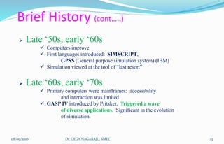
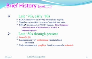
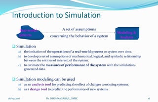
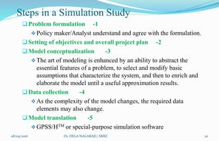
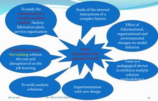
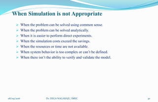
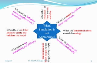
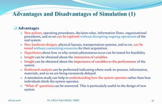
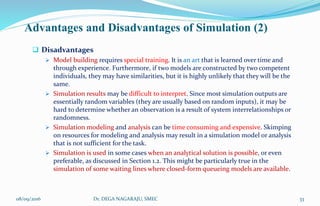
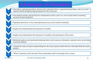
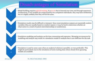
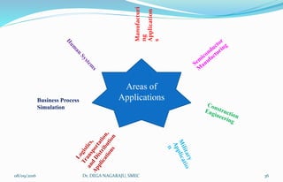
Simulation UNIT-I

SIMULATION
08/09/2016 1Dr. DEGA NAGARAJU, SMEC

08/09/2016 Dr. DEGA NAGARAJU, SMEC 2

08/09/2016 Dr. DEGA NAGARAJU, SMEC 3
War gaming: test
strategies; training
Flight Simulator
Transportation systems:
Improved operations; urban
planning
Computer communicationParallel computer systems:
Games
A few more applications …
12/22/2016 3Dr. DEGA NAGARAJU, SMBS

Areas of
Applications
Manufacturi
ng
Application
s
Business Process
Simulation

Applications:
 COMPUTER SYSTEMS: hardware components, software
systems, networks, data base management, information
processing, etc..
 MANUFACTURING: material handling systems, assembly
lines, automated production facilities, inventory control
systems, plant layout, etc..
 BUSINESS: stock and commodity analysis, pricing policies,
marketing strategies, cash flow analysis, forecasting, etc..
 GOVERNMENT: military weapons and their use, military
tactics, population forecasting, land use, health care
delivery, fire protection, criminal justice, traffic control, etc..
And the list goes on and on...

Examples of Applications at Disney World
 Cruise Line Operation: Simulate the arrival and
check-in process at the dock.
 Private Island Arrival: How to transport passengers
to the beach area? Drop-off point far from the
beach. Used simulation to determine whether
to invest in trams, how many trams to purchase,
average transport and waiting times, etc..

Why do we
go for
simulation
?
Is it possible to
represent all real
life problems
mathematically?
Method of
last resort
Logical
extension to
the analytical
&
mathematical
techniques
John Von Neumann &
Stanislaw Ulam
Nuclear Shielding
problem
1950-Digital Computers
Managerial decision
making
Aircraft-wind tunnel-
aerodynamic
characteristics
Scale models of
machines-plant layout
Pilot training-flight
simulator
Car Manufacturing
Simulation
TV games(chess playing
game, snake and
ladders)08/09/2016 7Dr. DEGA NAGARAJU, SMEC

Why do
we go for
simulati-
on?
Draw backs
of scientific
methods?
Draw backs of
Analytical
methods?
Draw backs of
iterative
methods?
Certain processes : too costly or impossible
Difficult-mathematical equations
No straight forward analytical solution
Ex: Queuing problems, Job shop problems,
Multi-integral problems etc.
Difficulty in performing validating
experiments for mathematical models
Dynamic programming, queuing theory,
network models
Dynamic programming-optimal strategies-
uncertainties-analyze multi-planning
problems
DP-simple cases-less number of static
variables
LPP-data does not change over the entire
planning horizon
One time decision process-average values for
decision variables
Many real life situations-uncertainties

Webster’s Dictionary:
“ to assume the mere appearance of ,
without the reality”

Definition:
Simulation is the process of designing a
model of a real system and conducting
experiments with this model for the purpose
of either understanding the behavior of the
system and/or evaluating various strategies
for the operation of the system.

Allows us to:
Model complex systems in a detailed way
Describe the behavior of systems
Construct theories or hypotheses that account for
the observed behavior
Use the model to predict future behavior, that is,
the effects that will be produced by changes in the
system
Analyze proposed systems

Brief History Not a very old technique...
 World War II
 “Monte Carlo” simulation: originated with
the work on the atomic bomb. Used to
simulate bombing raids. Given the
security code name “Monte-Carlo”.
 Still widely used today for certain problems
which are not analytically solvable (for
example: complex multiple integrals…)

Brief History (cont…..)
 Late ‘50s, early ‘60s
 Computers improve
 First languages introduced: SIMSCRIPT,
GPSS (General purpose simulation system) (IBM)
 Simulation viewed at the tool of “last resort”
 Primary computers were mainframes: accessibility
and interaction was limited
 GASP IV introduced by Pritsker. Triggered a wave
of diverse applications. Significant in the evolution
of simulation.

Brief History (cont…….)
 SLAM introduced in 1979 by Pritsker and Pegden.
 Models more credible because of sophisticated tools.
 SIMAN introduced in 1982 by Pegden. First language
to run on both a mainframe as well as a
microcomputer.
 Late ‘80s through present
 Powerful PCs
 Languages are very sophisticated (market almost
saturated)
 Major advancement: graphics. Models can now be animated.

What can be simulated?
Almost anything can
and
almost everything has...

Introduction to Simulation
 Simulation
a) the imitation of the operation of a real-world process or system over time.
b) to develop a set of assumptions of mathematical, logical, and symbolic relationship
between the entities of interest, of the system.
c) to estimate the measures of performance of the system with the simulation-
generated data.
 Simulation modeling can be used
a) as an analysis tool for predicting the effect of changes to existing systems.
b) as a design tool to predict the performance of new systems .
Real-world
process concerning the behavior of a system
A set of assumptions
Modeling &
Analysis

Simula-
tion
Imitation of the
operation of a real
world process
Whether done by
hand or on a
Computer
It involves
1. The generation of
an artificial history
of a system &
2. The observation of
that artificial
history
Simulation
model
Behavior of a
system
Set of Assumptions:
Mathematical, Logical,
Symbolic relationships
b/w entities, Objects of
interest
Used as:
an analysis tool,
a design tool

Simulation
Models
Solved by:
Differential Calculus,
Probability Theory,
Algebraic Methods
Solution Consists:
One or more numerical
parameters(Measures of
Performance)
Complex real world
systems:
Numerical computer
based simulation

Problem formulation -1
Policy maker/Analyst understand and agree with the formulation.
Setting of objectives and overall project plan -2
Model conceptualization -3
The art of modeling is enhanced by an ability to abstract the
essential features of a problem, to select and modify basic
assumptions that characterize the system, and then to enrich and
elaborate the model until a useful approximation results.
Data collection -4
As the complexity of the model changes, the required data
elements may also change.
Model translation -5
GPSS/HTM or special-purpose simulation software
Steps in a Simulation Study

Verified? -6
Is the computer program performing properly?
Debugging for correct input parameters and logical structure
Validated? -7
The determination that a model is an accurate representation of
the real system.
Validation is achieved through the calibration of the model
Experimental design -8
The decision on the length of the initialization period, the length
of simulation runs, and the number of replications to be made of
each run.
Production runs and analysis -9
To estimate measures of performances
Steps in a Simulation Study (Contd….)

More runs? -10
Documentation and reporting -11
Program documentation : for the relationships between input
parameters and output measures of performance, and for a
modification
Progress documentation : the history of a simulation, a
chronology of work done and decision made.
Implementation -12

Four phases according to Figure 1.3
First phase : a period of discovery or orientation
(step 1, step2)
Second phase : a model building and data collection
(step 3, step 4, step 5, step 6, step 7)
Third phase : running the model
(step 8, step 9, step 10)
Fourth phase : an implementation
(step 11, step 12)

The basic nature of Simulation
Two problems
Continuous
Discrete
State changes continuously
with time
Deterministic in nature
Arrival & Sale of Merchandise
occur in discrete steps
Stochastic in nature
Common
features
essential to
simulation
Common features:
Mathematical model of the system under study
Change of the state in accordance with some equations (rules or laws) for a
long period
Collection of information about the system (solution to the problem)
Programming the calculations for a digital computer
Simulate or mimic the real system with the help of computer
Continue the process until the desired analytic solution is obtained

Simulation as an analytic tool is useful only when done on a computer
The basic nature of Simulation (Cont….)
 Simulation of Inventory control manually Pencil and paper
System which can be simulated on a digital computer
Can also be simulated manually


Each application of Simulation is adhoc to a great extent
Simulation is an art
The basic nature of Simulation (Cont….)
No unifying theory of computer simulation
No unified theory No fundamental theorems
No underlying principles

Experimental technique
To simulate is to experiment Fast and inexpensive method
Ex: Inventory control problem






When Simulation is the Appropriate Tool (1)
 Simulation enables the study of, and experimentation with, the internal interactions
of a complex system, or of a subsystem within a complex system.
 Informational, organizational, and environmental changes can be simulated, and the
effect of these alterations on the model’s behavior can be observed.
 The knowledge gained in designing a simulation model may be of great value
toward suggesting improvement in the system under investigation.
 By changing simulation inputs and observing the resulting outputs, valuable insight
may be obtained into which variables are most important and how variables interact.
 Simulation can be used as a pedagogical device to reinforce analytic solution
methodologies.

 Simulation can be used to experiment with new designs or policies prior to
implementation, so as to prepare for what may happen.
 Simulation can be used to verify analytic solutions.
 By simulating different capabilities for a machine, requirements can be
determined.
 Simulation models designed for training allow learning without the cost and
disruption of on-the-job learning.
 Animation shows a system in simulated operation so that the plan can be
visualized.
 The modern system (factory, wafer fabrication plant, service organization, etc.)
is so complex that the interactions can be treated only through simulation.
When Simulation is the Appropriate Tool (2)

When
Simulation is the
appropriate tool?
Study of the internal
interactions of a
complex System
Effect of
Informational,
organizational and
environmental
changes on model
behavior
Used as a
pedagogical device
to reinforce analytic
solution
methodologies
Experimentation
with new design
To verify analytic
solutions
Simulation models:
For training without
the cost and
disruption of on the
job learning
To study the
interactions of a
complex modern
systems: factory,
fabrication plant,
service organization

When Simulation is not Appropriate
 When the problem can be solved using common sense.
 When the problem can be solved analytically.
 When it is easier to perform direct experiments.
 When the simulation costs exceed the savings.
 When the resources or time are not available.
 When system behavior is too complex or can’t be defined.
 When there isn’t the ability to verify and validate the model.

When
Simulation is
not
Appropriate?
Whentheproblem
canbesolvedusing
commonsenseWhenthe
resourcesor
timearenot
available
When there is n’t the
ability to verify and
validate the model
When the simulation costs
exceed the savings

Advantages and Disadvantages of Simulation (1)
 Advantages
 New polices, operating procedures, decision rules, information flows, organizational
procedures, and so on can be explored without disrupting ongoing operations of the
real system.
 New hardware designs, physical layouts, transportation systems, and so on, can be
tested without committing resources for their acquisition.
 Hypotheses about how or why certain phenomena occur can be tested for feasibility.
 Insight can be obtained about the interaction of variables.
 Insight can be obtained about the importance of variables to the performance of the
system.
 Bottleneck analysis can be performed indicating where work-in-process, information,
materials, and so on are being excessively delayed.
 A simulation study can help in understanding how the system operates rather than how
individuals think the system operates.
 “What-if” questions can be answered. This is particularly useful in the design of new
system.

Advantages and Disadvantages of Simulation (2)
 Disadvantages
 Model building requires special training. It is an art that is learned over time and
through experience. Furthermore, if two models are constructed by two competent
individuals, they may have similarities, but it is highly unlikely that they will be the
same.
 Simulation results may be difficult to interpret. Since most simulation outputs are
essentially random variables (they are usually based on random inputs), it may be
hard to determine whether an observation is a result of system interrelationships or
randomness.
 Simulation modeling and analysis can be time consuming and expensive. Skimping
on resources for modeling and analysis may result in a simulation model or analysis
that is not sufficient for the task.
 Simulation is used in some cases when an analytical solution is possible, or even
preferable, as discussed in Section 1.2. This might be particularly true in the
simulation of some waiting lines where closed-form queueing models are available.

1
• New polices, operating procedures, decision rules, information flows, organizational procedures, and so on can be
explored without disrupting ongoing operations of the real system
2
• New hardware designs, physical layouts, transportation systems, and so on, can be tested without committing
resources for their acquisition.
3
• Hypotheses about how or why certain phenomena occur can be tested for feasibility.
4
• Insight can be obtained about the interaction of variables.
5
• Insight can be obtained about the importance of variables to the performance of the system.
6
• Bottleneck analysis can be performed indicating where work-in-process, information, materials, and so on are being
excessively delayed
7
• A simulation study can help in understanding how the system operates rather than how individuals think the system
operates.
8
• “What-if” questions can be answered. This is particularly useful in the design of new system.
Advantages of Simulation

1
• Model building requires special training. It is an art that is learned over time and through experience.
Furthermore, if two models are constructed by two competent individuals, they may have similarities,
but it is highly unlikely that they will be the same.
2
• Simulation results may be difficult to interpret. Since most simulation outputs are essentially random
variables (they are usually based on random inputs), it may be hard to determine whether an
observation is a result of system interrelationships or randomness.
3
• Simulation modeling and analysis can be time consuming and expensive. Skimping on resources for
modeling and analysis may result in a simulation model or analysis that is not sufficient for the task.
4
• Simulation is used in some cases when an analytical solution is possible, or even preferable. This
might be particularly true in the simulation of some waiting lines where closed-form queueing
models are available.
Disadvantages of Simulation

Areas of
Applications
Manufacturi
ng
Application
s
Business Process
Simulation

Why do we
study the
System?
To understand the relationships b/w its
components or to predict how the system will
operate under a new policy
Is it possible to
conduct experiment
with the system?
Yes, but not always
New system may not yet exist. It may
be in hypothetical form or at the
design stage.
Example: Developing & testing of
prototype models can be very
expensive and time consuming
Even System exists: No
experimentation.
Example:
Is it possible to double the
unemployment rate to determine the
effect of employment on inflation?
Is it possible to reduce the number of
tellers at the bank to study the effect
on the length of waiting lines?
Is it feasible to change the supply and
demand of goods arbitrarily to study
the economic systems?
How do we
define the
system
model?
Body of information gathered about
the system to study the system.
No unique model of the system
For same system-different models-by
different analysts
Establish the model
Structure: System boundary,
entities, attributes and
activities of the system.
Provide the data: Values of
the attributes, relationships
among the activities.
MODEL OF A SYSTEM
How the model
is derived for
the system?

Example for the Model of a System
ENTITY ATTRIBUTE ACTIVITY
SHOPPER NO OF ITEMS
ARRIVE
GET
BASKET AVAILABILITY
SHOP
QUEUE
CHECK-OUT
COUNTER NUMBER OF
OCCUPANCY
RETURN
LEAVE
Elements of a Super Market

Types of models
Physical
Static Dynamic
Mathematical
Static
Numerical Analytical
Dynamic
Analytical Numerical
System
Simulation
TYPES OF MODELS

Physical Models:
Based on some analogy b/w such systems as
mechanical & electrical, electrical & hydraulic
System attributes represented by such
measurements as a voltage or the position of a
shaft
System activities are reflected in the physical
laws that drive the model:
Example: amount of voltage applied – speed of
the shaft of the motor
Voltage applied – Velocity of the vehicle
Number of revolutions of the shaft – distance
traveled by the vehicle
Mathematical
Models:
Used symbolic notations, mathematical equations
etc.
System attributes are represented by variables
System activities are represented by mathematical
functions

Dynamic Models:
Static Models:
Also called as Monte Carlo Simulation
Represents the system at a particular point in time
Represents systems as they change over time
Example: Simulation of a bank from 9.00 am to
4.00 pm
Numerical Models:
Analytical Models: Only certain forms of equations are solved
Example: Linear differential equations are solved
Computational procedure is used to solve the
models

Monte Carlo Simulation
Statistical distribution functions are created by using a
series of random numbers.
Data can be developed for many months or years in a
matter of few minutes on a digital computer.
Used to solve the problems which can’t be adequately
represented by mathematical models or where
the solution of the model is not possible by
analytical method.
The solution obtained is very close to the optimal but
not exact.

Steps in Monte
Carlo Simulation
Objectives,
factors affecting
the objectives
Variables, parameters, decision rules,
conditions to carry experimentation, type of
distribution used, the manner in which time
is changed, relationship b/w variables and
parameters
Starting conditions
for the simulation,
number of
simulation runs
Define a coding system that will
correlate the factors defined in step
1 with random numbers to be
generated;
Select the random number generator and create
the random numbers to be used;
Associate the generated random numbers with
the factors identified in step 1 and coded in step
4(i)
Select the best
course of action

Systems and System Environment
 System
 defined as a group of objects that are joined together in some regular
interaction or interdependence toward the accomplishment of some
purpose.
 System Environment
 changes occurring outside the system.
 The decision on the boundary between the system and its environment
may depend on the purpose of the study.

Components of a System
 Entity : an object of interest in the system.
 Attribute : a property of an entity.
 Activity : a time period of specified length.
 State : the collection of variables necessary to describe the
system at any time, relative to the objectives of the
study.
 Event : an instantaneous occurrence that may change the
state of the system.
 Endogenous : to describe activities and events occurring
within a system.
 Exogenous : to describe activities and events in an
environment that affect the system.

Components of a System

Discrete and Continuous Systems
 Systems can be categorized as discrete or continuous.
 Bank : a discrete system
 The head of water behind a dam : a continuous system

DISCRETE SYSTEMS
State variables change only at a discrete set of points in
time
Example: Bank
State variable: Number of customers in the
bank
Note: The state variable changes only when a new
customer arrives or when the service provided to the
customer is completed

CONTINUOUS SYSTEMS
State variables change continuously over time
Example: Head of water behind a dam
State variable: Head of water behind a dam
Note: During and for some time after a rain storm,
water flows into the lake behind the dam. Water is
drawn from the dam for flood control and to make
electricity. Evaporation also decreases the water level.

A grocery store has one checkout counter. Customers arrive at this checkout counter at
random from 1 to 8 minutes apart and each interval time has the same probability of
occurrence. The service times vary from 1 to 6 minutes, with probability given below:
Simulate the arrival of 6 customers and calculate (i) Average waiting time for a customer,
(ii) Probability that a customer has to wait, (iii) Probability of a server being idle (iv)
Average service time, (v) Average time between arrival. Use the following sequence of
random numbers:
Assume the first customer arrives at time θ. Depict the simulation in a tabular form.
Service (minutes) 1 2 3 4 5 6
Probability 0.10 0.20 0.30 0.25 0.10 0.05
Random digit for
arrival
913 727 015 948 309 922
Random digit for
service time
84 10 74 53 17 79

Time between
arrivals
Probability Cumulative
Probability
Random digit
assignment
1 0.125 0.125 001-125
2 0.125 0.250 126-250
3 0.125 0.375 251-375
4 0.125 0.500 376-500
5 0.125 0.625 501-625
6 0.125 0.750 626-750
7 0.125 0.875 751-875
8 0.125 1.000 876-000
ARRIVAL TIME DISTRIBUTION
Arrival time varies from 1 to 8 minutes with equal probability, meaning that
the probability of each arrival = 1/8 = 0.125

Service Time Probability
Cumulative
Probability
Random digit
assignment
1 0.10 0.10 01-10
2 0.20 0.30 11-30
3 0.30 0.60 31-60
4 0.25 0.85 61-85
5 0.10 0.95 86-95
6 0.05 1.00 96-00
SERVICE TIME DISTRIBUTION

Custom
er
Random
No. for
Arrival
Time
since
last
arrival
Arrival
time
Random
No. for
Service
Service
time
Time
service
begins
Time
custome
-r waits
in queue
Time
service
ends
Time
custome
r spends
in
system
Idle
time of
server
1 - - 0 84 4 0 0 4 4 0
2 913 8 8 10 1 8 0 9 1 4
3 727 6 14 74 4 14 0 18 4 5
4 015 1 15 53 3 18 3 21 6 0
5 948 8 23 17 2 23 0 25 2 2
6 309 3 26 79 4 26 0 30 4 1
18 3 21 12
SIMULATION TABLE

 Total time customer waits in queue 3Average waiting 0.5
time for customer Total no. of customers 6
  
 No. of customers who wait 1Pr obability that a 0.166
customer has to wait Total no. of customers 6
  
 Total idle time of server 12Pr obability of server 0.4
being idle Total run time of system 30
  
 Total service time 18Average service 3
time Total no. of customer 6
  
 Sum of all times between arrivals(min utes) 26Average time between
arrivals No. of arrivals 1 6 1
 
 

 Total timecustomers wait in queue(min utes)Average waiting time of those
whowait(min utes) Totalnumber of customers who wait
3
3min utes
1

 

Total timecustomer spends
in the system(min utes)Average time customer spends
in the system Totalnumber of customers
21
3.5min utes
6

 

Demand
(daily)
0 1 2 3 4
Probability 0.05 0.10 0.30 0.45 0.10
A book store wishes to carry ‘Ramayana’ in stock. Demand is probabilistic and
replenishment of stock takes 2 days (i.e., if an order is placed on March 1, it will be
delivered at the end of the day on March 3). The probabilities of demand are given
below:
Each time an order is placed, the store incurs an ordering cost of Rs. 10 per order.
The store also incurs a carrying cost of Rs. 0.50 per book per day. The inventory
carrying cost is calculated on the basis of stock at the time of each day. The manager
of the book store wishes to compare two options for his inventory decision.
A: Order 5 books when the inventory at the beginning of the day plus order
outstanding is less than 8 books.
B: Order 8 books when the inventory at the beginning of the day plus order
outstanding is less than 8.
Currently (beginning of the first day) the store has stock of 8 books plus 6 books
ordered 2 days ago and expected to arrive next day. Using Monte-Carlo Simulation
for 10 cycles, recommend which option the manager should choose. The two digit
random numbers are given below. 89, 34, 78, 63, 61, 81, 39, 16, 13, 73.

Demand Prob. Cum. Prob.
Random
Nos.
0 0.05 0.05 01-05
1 0.10 0.15 06-15
2 0.30 0.45 16-45
3 0.45 0.90 46-90
4 0.10 1.00 91-00
Stock in hand = 8, and
stock on order = 6 (expected next day).
Demand Distribution

Random
No.
Demand
sales
Opt. stock
in hand
Receipt
Cl. stock
in hand
Opt. stock
on order
Order
Qty.
Cl. Stock
on order
89 3 8 - 5 6 - 6
34 2 5 6 9 - - -
78 3 9 - 6 - 5 5
63 3 6 - 3 5 - 5
61 3 3 - 0 5 5 10
81 3 0 5 2 5 5 10
39 2 2 - 0 10 - 10
16 2 0 5 3 5 - 5
13 1 3 5 7 0 5 5
73 3 7 - 4 5 - 5
No. of orders =4 Ordering cost = 4 x 10 = Rs. 40.
Closing stock of 10 days = 39, Carrying cost = 39 x 0.50 = 19.50
Cost for 10 days = 59.50
OPTION A

OPTION B
Random
No.
Demand
sales
Opt. stock
in hand
Receipt
Cl. stock
in hand
Opt. stock
on order
Order
Qty.
Cl. Stock
on order
89 3 8 - 5 6 - 6
34 2 5 6 9 - - -
78 3 9 - 6 - 8 8
63 3 6 - 3 8 - 8
61 3 3 - 0 8 - 8
81 3 0 8 5 - 8 8
39 2 5 - 3 8 - 8
16 2 3 - 1 8 - 8
13 1 1 8 8 - - -
73 3 8 - 5 - 8 8
No. of orders =3 Ordering cost = 3 x 10 = Rs. 30.
Closing stock of 10 days = 45, Carrying cost = 45 x 0.50 = 22.50
Cost for 10 days = 52.50
Since, option B has lower cost, manager should choose option B

 Discrete-event simulation (General Principles)
 The basic building blocks of all discrete-event simulation models
: entities and attributes, activities and events.
 A system is modeled in terms of
 its state at each point in time
 the entities that pass through the system and the entities that represent
system resources
 the activities and events that cause system state to change.
 Discrete-event models are appropriate for those systems for which changes in
system state occur only at discrete points in time.
 This chapter deals exclusively with dynamic, stochastic systems (i.e.,
involving time and containing random elements) which change in a discrete
manner.08/09/2016 60Dr. DEGA NAGARAJU, SMEC

 System : A collection of entities (e.g., people and machines) that interact
together over time to accomplish one or more goals.
 Model : An abstract representation of a system, usually containing
structural, logical, or mathematical relationships which describe a
system in terms of state, entities and their attributes, sets, processes,
events, activities, and delays.
 System state : A collection of variables that contain all the information
necessary to describe the system at any time.
 Entity : Any object or component in the system which requires explicit
representation in the model (e.g., a server, a customer, a machine).
 Attributes : The properties of a given entity (e.g., the priority of a waiting
customer, the routing of a job through a job shop).

 List : A collection of (permanently or temporarily) associated entities, ordered
in some logical fashion (such as all customers currently in a waiting line,
ordered by first come, first served, or by priority).
 Event : An instantaneous occurrence that changes the state of a system
(such as an arrival of a new customer).
 Event notice : A record of an event to occur at the current or some future
time, along with any associated data necessary to execute the
event; at a minimum, the record includes the event type and
the event time.
 Event list : A list of event notices for future events, ordered by time of
occurrence also known as the future event list (FEL).
 Activity : A duration of time of specified length (e.g., a service time or
inter arrival time), which is known when it begins (although it may be
defined in terms of a statistical distribution).

 Delay : A duration of time of unspecified indefinite length, which is not
known until it ends (e.g., a customer's delay in a last-in, first-out
waiting line which, when it begins, depends on future arrivals).
 Clock : A variable representing simulated time, called CLOCK in the
examples to follow.
 An activity typically represents a service time, an inter arrival time, or any other
processing time whose duration has been characterized and defined by the modeler.
 An activity's duration may be specified in a number of ways:
 1. Deterministic-for example, always exactly 5 minutes;
 2. Statistical-for example, as a random draw from among 2, 5, 7 with equal
probabilities;
 3. A function depending on system variables and/or entity attributes-for example,
loading time for an iron ore ship as a function of the ship's allowed cargo
weight and the loading rate in tons per hour.

Simulation UNIT-I

More Related Content

What's hot

Similar to Simulation UNIT-I

Recently uploaded

Simulation UNIT-I