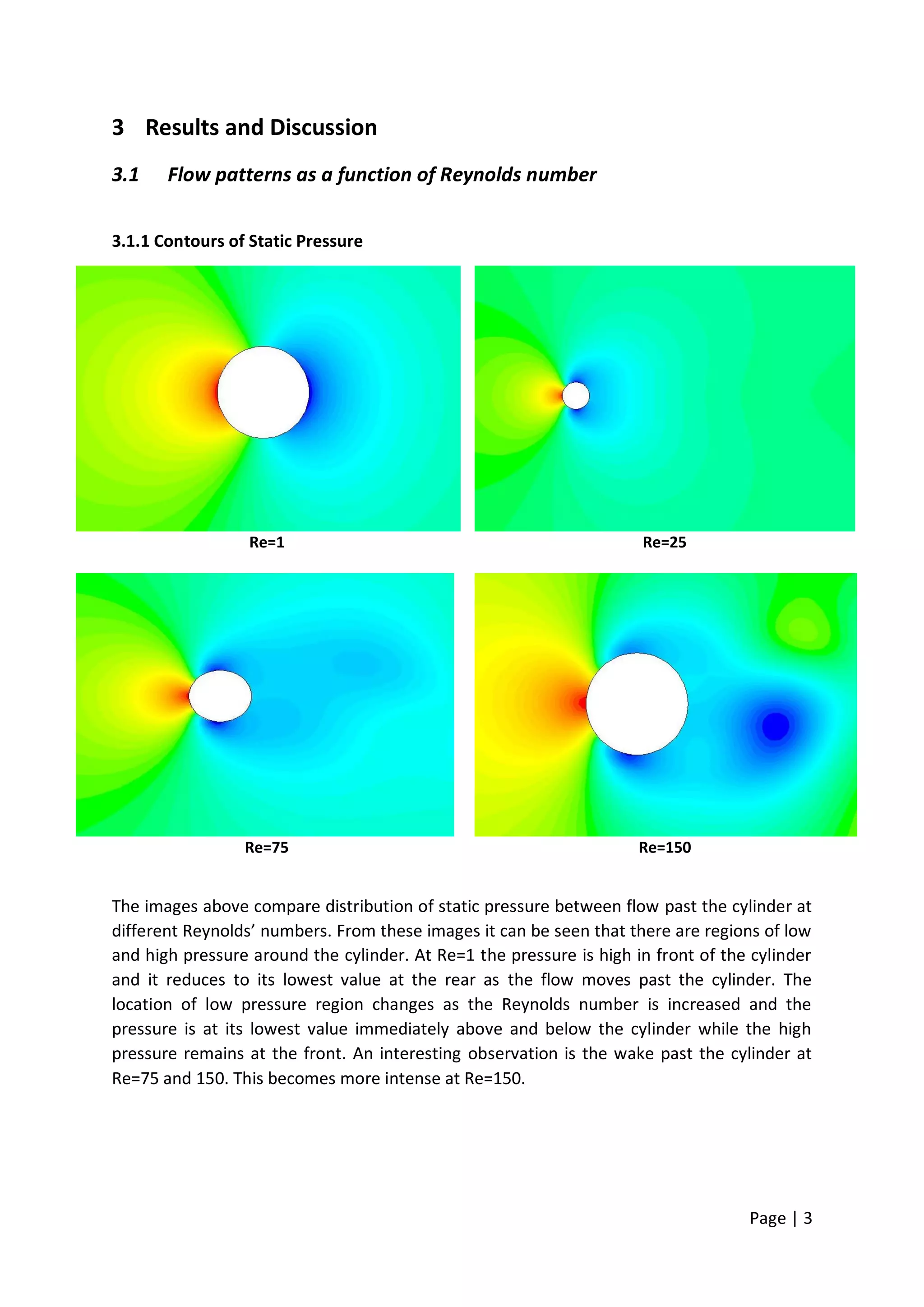
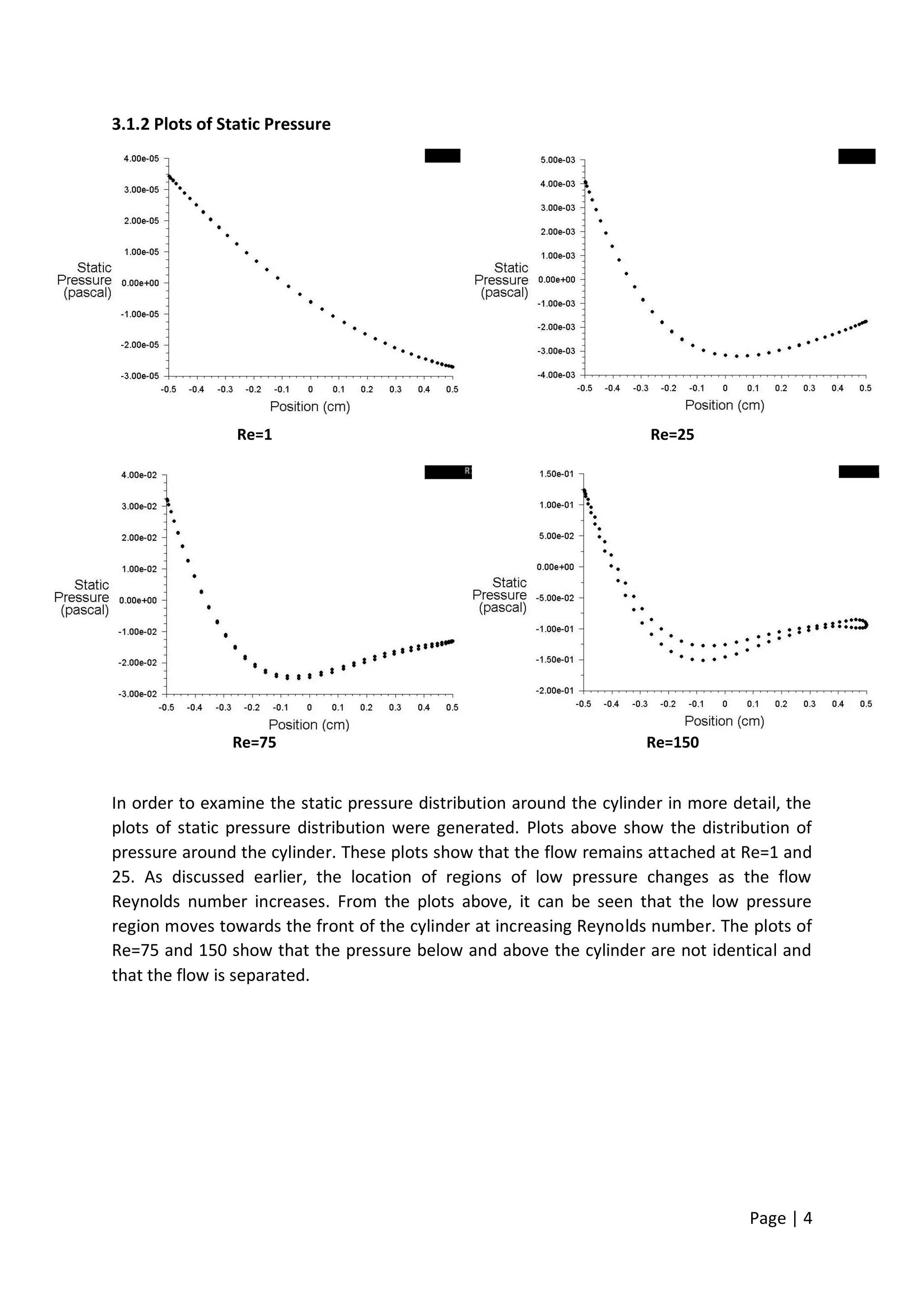
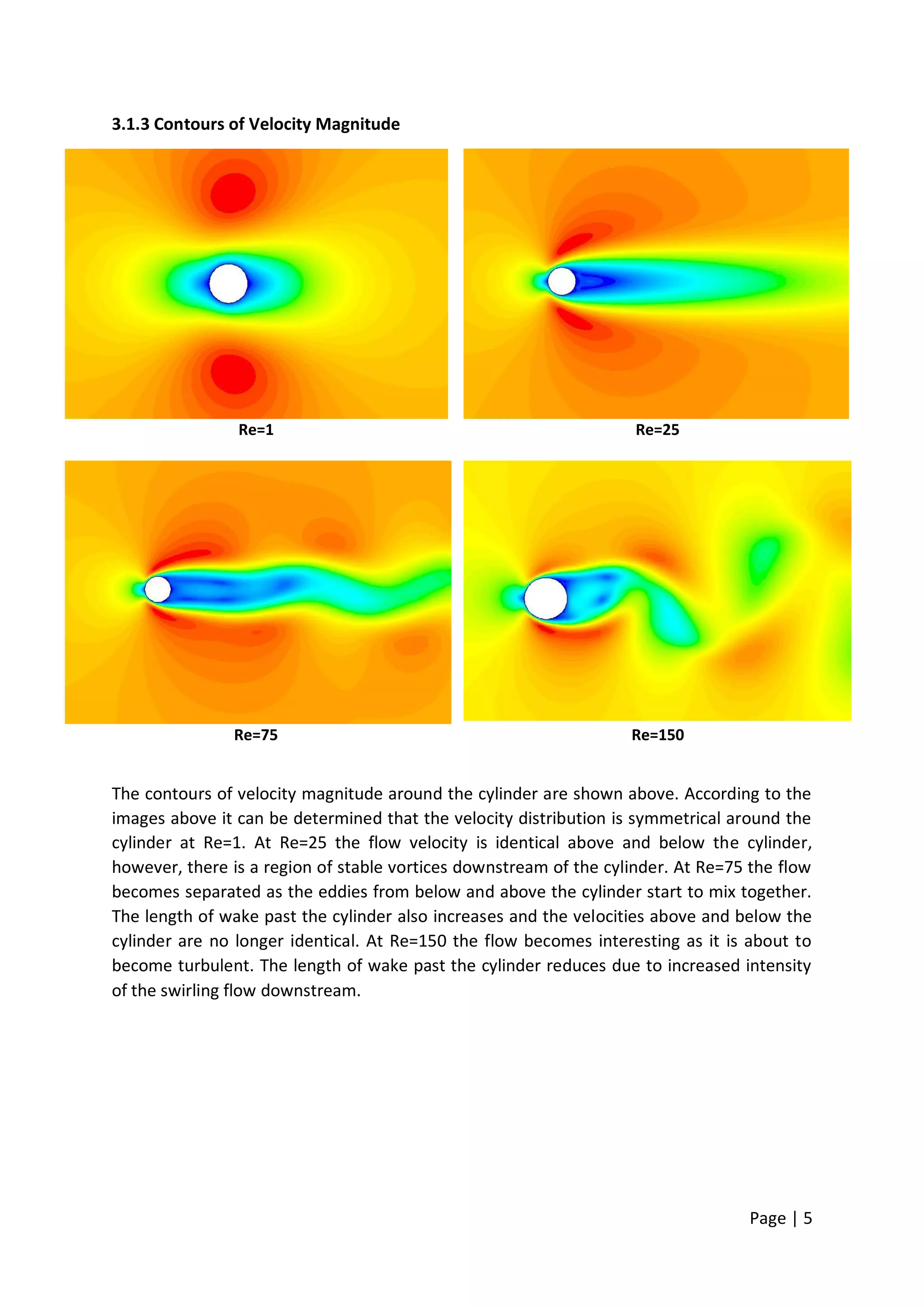
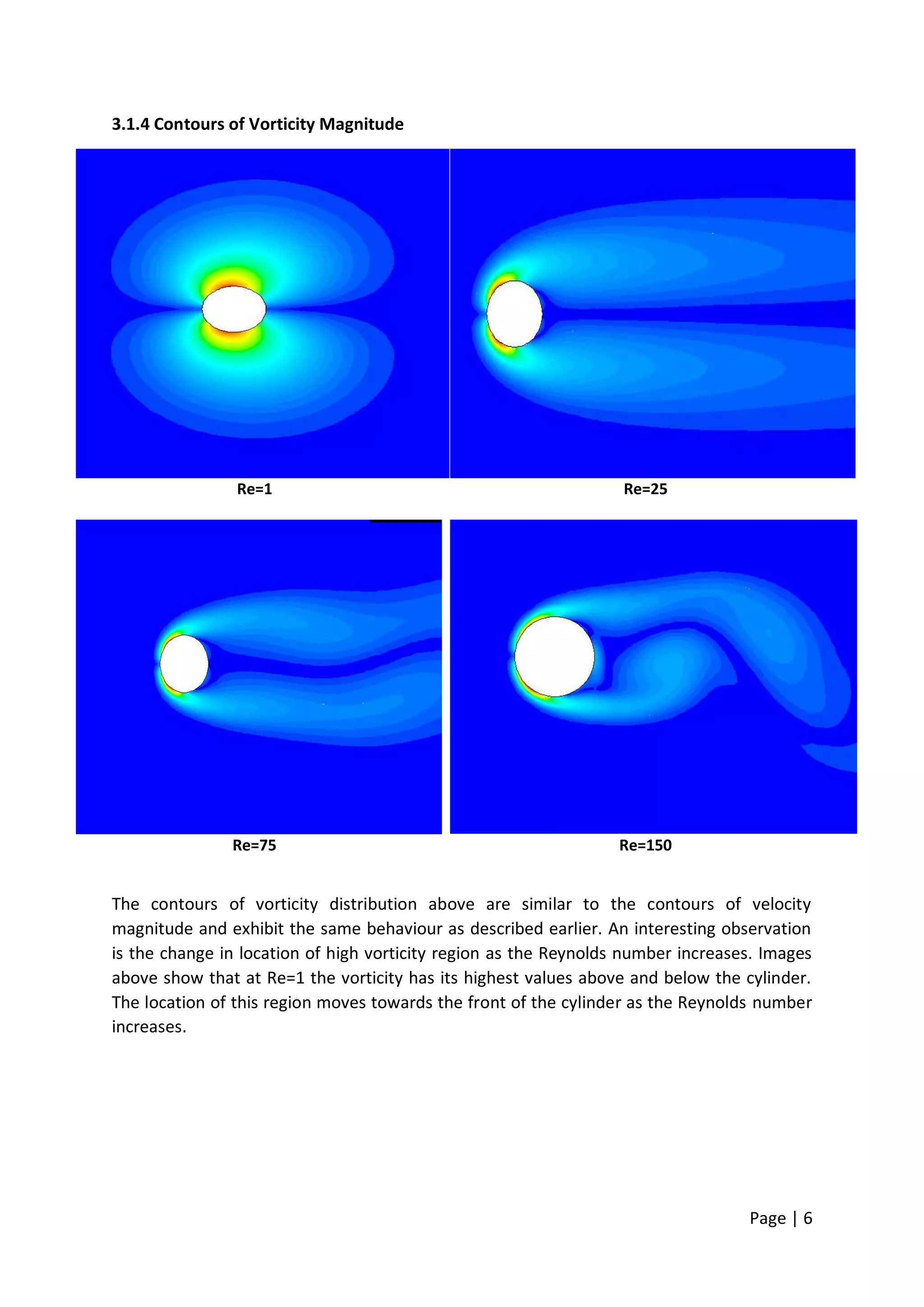
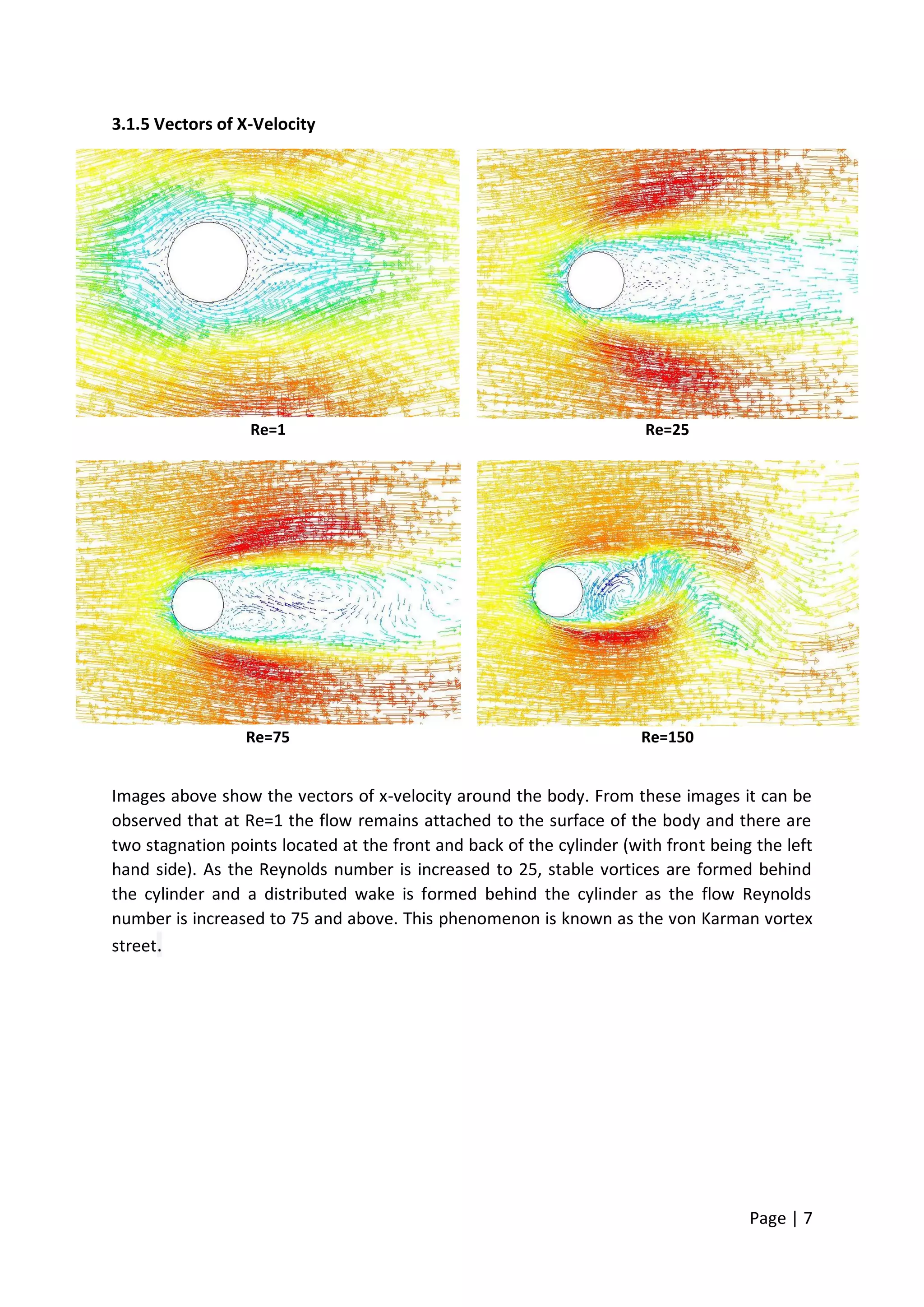
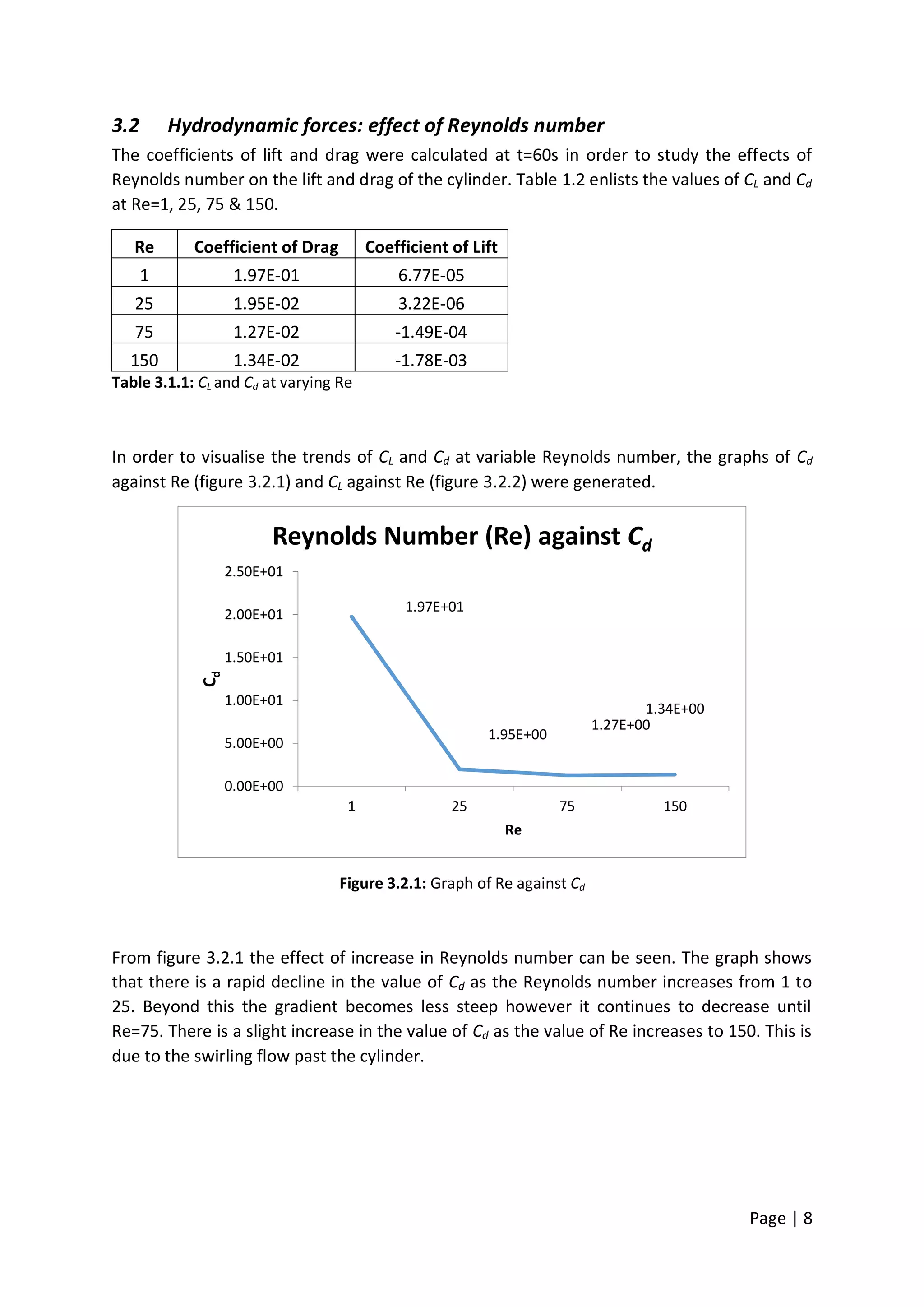
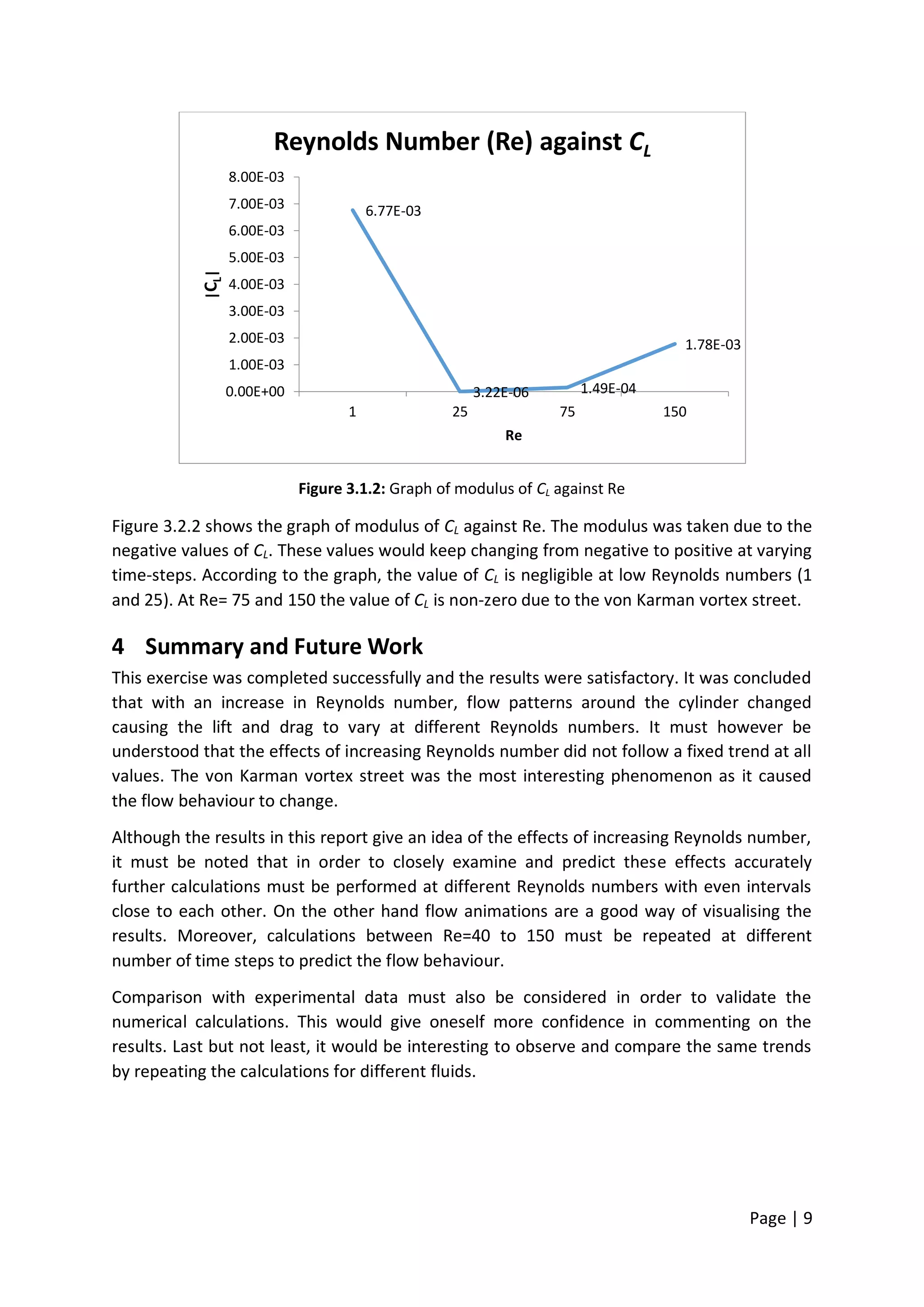
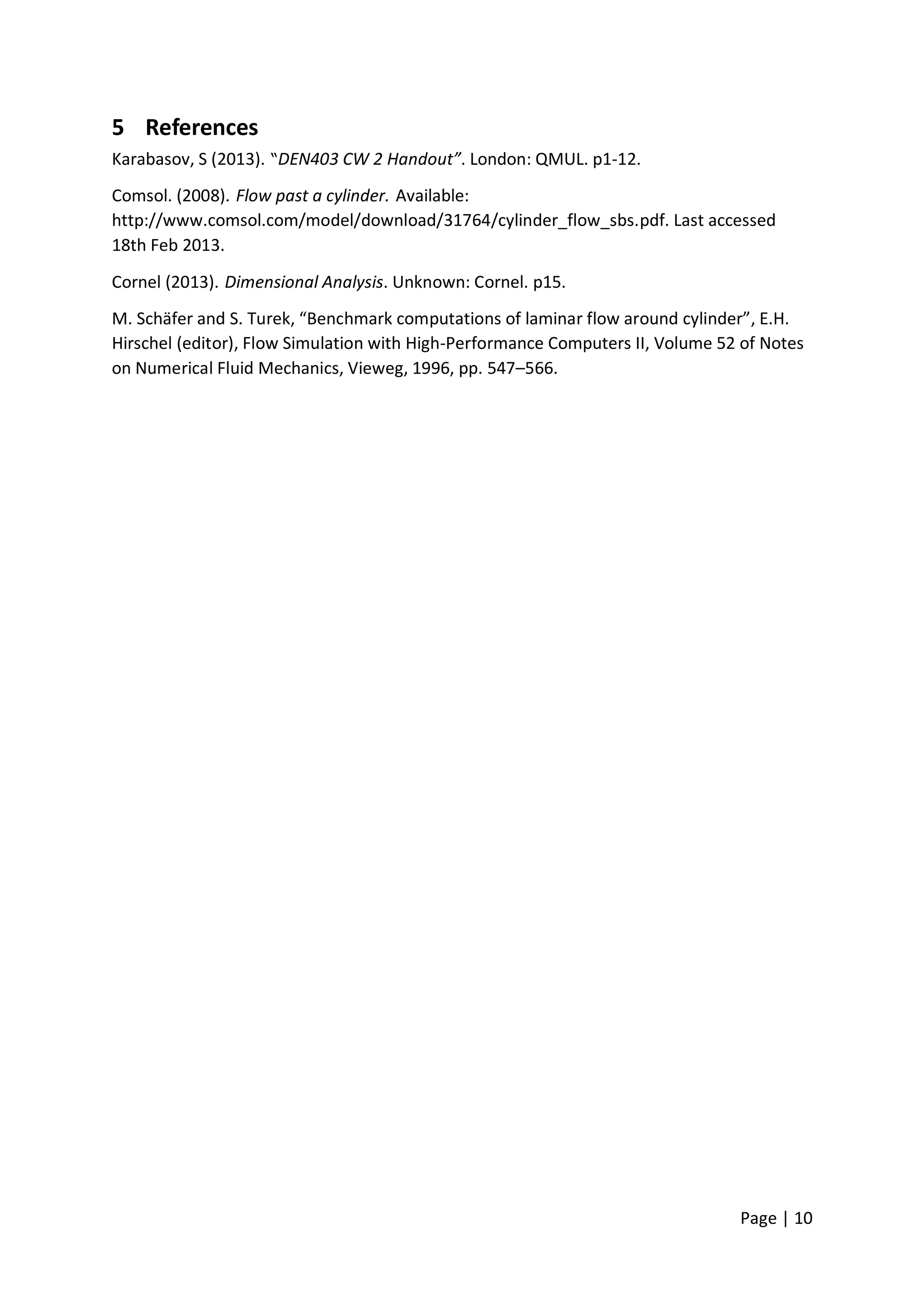
Simulation of flow past
cylinder at moderate
Reynolds numbers
Computational Fluid Dynamics
Author: Mr. Shahzaib Malik
Page | 1
Table of Contents
1 Introduction................................................................................................................... 2
2 Numerical Method......................................................................................................... 2
3 Results and Discussion ................................................................................................... 3
3.1 Flow patterns as a function of Reynolds number..................................................... 3
3.2 Hydrodynamic forces: effect of Reynolds number................................................... 8
4 Summary and Future Work ............................................................................................ 9
5 References................................................................................................................... 10
Page | 2
1 Introduction
The study of flow around cylinder has been very helpful in examining the effects of Reynolds
number on the hydrodynamic forces acting on blunt bodies. It has numerous applications in
the fields of aerospace, marine and automobiles.
A significant amount of drag is produced as a consequence of placing a cylinder in laminar
flow field. This becomes more interesting as the Reynolds number is increased and the flow
starts to behave in a peculiar manner when eddies past a circular cylinder start to mix
together resulting in the formation of the von Karman vortex street (Comsol, 2008).
This report aims to study the effects of moderate Reynolds numbers on the flow behaviour
and magnitude of hydrodynamic forces acting on a two-dimensional cylinder of unit depth
using computational fluid dynamics. There are four physical parameters linked with this
problem: Viscosity, free stream velocity, characteristic length (diameter of the cylinder) and
density of the fluid (Cornel, 2013).
2 Numerical Method
In order to simulate the flow past a circular cylinder computational code “Fluent” version
14.5 was used. The grid was provided by Karabasov (2013) and transient time was used in
order to capture the unsteady flow using a pressure based solver. PISO coupling scheme was
used in order to discretise the flow problem. PISO comes from the SIMPLE algorithm range
and it provides higher order approximation as compared to SIMPLE scheme. The
convergence criterion for continuity, x-velocity and y- velocity were set to 1E-04 in order to
achieve a balance between computational time and precision. A time-step size of 0.2s was
used to capture the flow and the solution was calculated for 300 time-steps with a
maximum of 350 iterations per time-step.
Calculations were performed over a range of Re numbers between Re= 1 to 150. In order to
match the flow Reynolds number, density and viscosity were kept constant at 1000 kgm-3
and 0.001 kg/m.s respectively, while velocity was changed. Table 2.0.1 shows these
Reynolds numbers and corresponding velocities:
Re Velocity (ms-1)
1 1.0E-04
25 2.5E-03
75 7.5E-03
150 1.5E-02
Table 2.0.1: Reynolds numbers and corresponding velocities
Page | 3
3 Results and Discussion
3.1 Flow patterns as a function of Reynolds number
3.1.1 Contours of Static Pressure
Re=1 Re=25
Re=75 Re=150
The images above compare distribution of static pressure between flow past the cylinder at
different Reynolds’ numbers. From these images it can be seen that there are regions of low
and high pressure around the cylinder. At Re=1 the pressure is high in front of the cylinder
and it reduces to its lowest value at the rear as the flow moves past the cylinder. The
location of low pressure region changes as the Reynolds number is increased and the
pressure is at its lowest value immediately above and below the cylinder while the high
pressure remains at the front. An interesting observation is the wake past the cylinder at
Re=75 and 150. This becomes more intense at Re=150.
Page | 4
3.1.2 Plots of Static Pressure
Re=1 Re=25
Re=75 Re=150
In order to examine the static pressure distribution around the cylinder in more detail, the
plots of static pressure distribution were generated. Plots above show the distribution of
pressure around the cylinder. These plots show that the flow remains attached at Re=1 and
25. As discussed earlier, the location of regions of low pressure changes as the flow
Reynolds number increases. From the plots above, it can be seen that the low pressure
region moves towards the front of the cylinder at increasing Reynolds number. The plots of
Re=75 and 150 show that the pressure below and above the cylinder are not identical and
that the flow is separated.
Page | 5
3.1.3 Contours of Velocity Magnitude
Re=1 Re=25
Re=75 Re=150
The contours of velocity magnitude around the cylinder are shown above. According to the
images above it can be determined that the velocity distribution is symmetrical around the
cylinder at Re=1. At Re=25 the flow velocity is identical above and below the cylinder,
however, there is a region of stable vortices downstream of the cylinder. At Re=75 the flow
becomes separated as the eddies from below and above the cylinder start to mix together.
The length of wake past the cylinder also increases and the velocities above and below the
cylinder are no longer identical. At Re=150 the flow becomes interesting as it is about to
become turbulent. The length of wake past the cylinder reduces due to increased intensity
of the swirling flow downstream.
Page | 6
3.1.4 Contours of Vorticity Magnitude
Re=1 Re=25
Re=75 Re=150
The contours of vorticity distribution above are similar to the contours of velocity
magnitude and exhibit the same behaviour as described earlier. An interesting observation
is the change in location of high vorticity region as the Reynolds number increases. Images
above show that at Re=1 the vorticity has its highest values above and below the cylinder.
The location of this region moves towards the front of the cylinder as the Reynolds number
increases.
Page | 7
3.1.5 Vectors of X-Velocity
Re=1 Re=25
Re=75 Re=150
Images above show the vectors of x-velocity around the body. From these images it can be
observed that at Re=1 the flow remains attached to the surface of the body and there are
two stagnation points located at the front and back of the cylinder (with front being the left
hand side). As the Reynolds number is increased to 25, stable vortices are formed behind
the cylinder and a distributed wake is formed behind the cylinder as the flow Reynolds
number is increased to 75 and above. This phenomenon is known as the von Karman vortex
street.
Page | 8
3.2 Hydrodynamic forces: effect of Reynolds number
The coefficients of lift and drag were calculated at t=60s in order to study the effects of
Reynolds number on the lift and drag of the cylinder. Table 1.2 enlists the values of CL and Cd
at Re=1, 25, 75 & 150.
Re Coefficient of Drag Coefficient of Lift
1 1.97E-01 6.77E-05
25 1.95E-02 3.22E-06
75 1.27E-02 -1.49E-04
150 1.34E-02 -1.78E-03
Table 3.1.1: CL and Cd at varying Re
In order to visualise the trends of CL and Cd at variable Reynolds number, the graphs of Cd
against Re (figure 3.2.1) and CL against Re (figure 3.2.2) were generated.
Figure 3.2.1: Graph of Re against Cd
From figure 3.2.1 the effect of increase in Reynolds number can be seen. The graph shows
that there is a rapid decline in the value of Cd as the Reynolds number increases from 1 to
25. Beyond this the gradient becomes less steep however it continues to decrease until
Re=75. There is a slight increase in the value of Cd as the value of Re increases to 150. This is
due to the swirling flow past the cylinder.
1.97E+01
1.95E+00
1.27E+00
1.34E+00
0.00E+00
5.00E+00
1.00E+01
1.50E+01
2.00E+01
2.50E+01
1 25 75 150
Cd
Re
Reynolds Number (Re) against Cd
Page | 9
Figure 3.1.2: Graph of modulus of CL against Re
Figure 3.2.2 shows the graph of modulus of CL against Re. The modulus was taken due to the
negative values of CL. These values would keep changing from negative to positive at varying
time-steps. According to the graph, the value of CL is negligible at low Reynolds numbers (1
and 25). At Re= 75 and 150 the value of CL is non-zero due to the von Karman vortex street.
4 Summary and Future Work
This exercise was completed successfully and the results were satisfactory. It was concluded
that with an increase in Reynolds number, flow patterns around the cylinder changed
causing the lift and drag to vary at different Reynolds numbers. It must however be
understood that the effects of increasing Reynolds number did not follow a fixed trend at all
values. The von Karman vortex street was the most interesting phenomenon as it caused
the flow behaviour to change.
Although the results in this report give an idea of the effects of increasing Reynolds number,
it must be noted that in order to closely examine and predict these effects accurately
further calculations must be performed at different Reynolds numbers with even intervals
close to each other. On the other hand flow animations are a good way of visualising the
results. Moreover, calculations between Re=40 to 150 must be repeated at different
number of time steps to predict the flow behaviour.
Comparison with experimental data must also be considered in order to validate the
numerical calculations. This would give oneself more confidence in commenting on the
results. Last but not least, it would be interesting to observe and compare the same trends
by repeating the calculations for different fluids.
6.77E-03
3.22E-06 1.49E-04
1.78E-03
0.00E+00
1.00E-03
2.00E-03
3.00E-03
4.00E-03
5.00E-03
6.00E-03
7.00E-03
8.00E-03
1 25 75 150
|CL|
Re
Reynolds Number (Re) against CL
Page | 10
5 References
Karabasov, S (2013). “DEN403 CW 2 Handout”. London: QMUL. p1-12.
Comsol. (2008). Flow past a cylinder. Available:
http://www.comsol.com/model/download/31764/cylinder_flow_sbs.pdf. Last accessed
18th Feb 2013.
Cornel (2013). Dimensional Analysis. Unknown: Cornel. p15.
M. Schäfer and S. Turek, “Benchmark computations of laminar flow around cylinder”, E.H.
Hirschel (editor), Flow Simulation with High-Performance Computers II, Volume 52 of Notes
on Numerical Fluid Mechanics, Vieweg, 1996, pp. 547–566.

Simulation of flow past cylinder at moderate Reynolds numbers

  • 1.
    Simulation of flowpast cylinder at moderate Reynolds numbers Computational Fluid Dynamics Author: Mr. Shahzaib Malik
  • 2.
    Page | 1 Tableof Contents 1 Introduction................................................................................................................... 2 2 Numerical Method......................................................................................................... 2 3 Results and Discussion ................................................................................................... 3 3.1 Flow patterns as a function of Reynolds number..................................................... 3 3.2 Hydrodynamic forces: effect of Reynolds number................................................... 8 4 Summary and Future Work ............................................................................................ 9 5 References................................................................................................................... 10
  • 3.
    Page | 2 1Introduction The study of flow around cylinder has been very helpful in examining the effects of Reynolds number on the hydrodynamic forces acting on blunt bodies. It has numerous applications in the fields of aerospace, marine and automobiles. A significant amount of drag is produced as a consequence of placing a cylinder in laminar flow field. This becomes more interesting as the Reynolds number is increased and the flow starts to behave in a peculiar manner when eddies past a circular cylinder start to mix together resulting in the formation of the von Karman vortex street (Comsol, 2008). This report aims to study the effects of moderate Reynolds numbers on the flow behaviour and magnitude of hydrodynamic forces acting on a two-dimensional cylinder of unit depth using computational fluid dynamics. There are four physical parameters linked with this problem: Viscosity, free stream velocity, characteristic length (diameter of the cylinder) and density of the fluid (Cornel, 2013). 2 Numerical Method In order to simulate the flow past a circular cylinder computational code “Fluent” version 14.5 was used. The grid was provided by Karabasov (2013) and transient time was used in order to capture the unsteady flow using a pressure based solver. PISO coupling scheme was used in order to discretise the flow problem. PISO comes from the SIMPLE algorithm range and it provides higher order approximation as compared to SIMPLE scheme. The convergence criterion for continuity, x-velocity and y- velocity were set to 1E-04 in order to achieve a balance between computational time and precision. A time-step size of 0.2s was used to capture the flow and the solution was calculated for 300 time-steps with a maximum of 350 iterations per time-step. Calculations were performed over a range of Re numbers between Re= 1 to 150. In order to match the flow Reynolds number, density and viscosity were kept constant at 1000 kgm-3 and 0.001 kg/m.s respectively, while velocity was changed. Table 2.0.1 shows these Reynolds numbers and corresponding velocities: Re Velocity (ms-1) 1 1.0E-04 25 2.5E-03 75 7.5E-03 150 1.5E-02 Table 2.0.1: Reynolds numbers and corresponding velocities
  • 4.
    Page | 3 3Results and Discussion 3.1 Flow patterns as a function of Reynolds number 3.1.1 Contours of Static Pressure Re=1 Re=25 Re=75 Re=150 The images above compare distribution of static pressure between flow past the cylinder at different Reynolds’ numbers. From these images it can be seen that there are regions of low and high pressure around the cylinder. At Re=1 the pressure is high in front of the cylinder and it reduces to its lowest value at the rear as the flow moves past the cylinder. The location of low pressure region changes as the Reynolds number is increased and the pressure is at its lowest value immediately above and below the cylinder while the high pressure remains at the front. An interesting observation is the wake past the cylinder at Re=75 and 150. This becomes more intense at Re=150.
  • 5.
    Page | 4 3.1.2Plots of Static Pressure Re=1 Re=25 Re=75 Re=150 In order to examine the static pressure distribution around the cylinder in more detail, the plots of static pressure distribution were generated. Plots above show the distribution of pressure around the cylinder. These plots show that the flow remains attached at Re=1 and 25. As discussed earlier, the location of regions of low pressure changes as the flow Reynolds number increases. From the plots above, it can be seen that the low pressure region moves towards the front of the cylinder at increasing Reynolds number. The plots of Re=75 and 150 show that the pressure below and above the cylinder are not identical and that the flow is separated.
  • 6.
    Page | 5 3.1.3Contours of Velocity Magnitude Re=1 Re=25 Re=75 Re=150 The contours of velocity magnitude around the cylinder are shown above. According to the images above it can be determined that the velocity distribution is symmetrical around the cylinder at Re=1. At Re=25 the flow velocity is identical above and below the cylinder, however, there is a region of stable vortices downstream of the cylinder. At Re=75 the flow becomes separated as the eddies from below and above the cylinder start to mix together. The length of wake past the cylinder also increases and the velocities above and below the cylinder are no longer identical. At Re=150 the flow becomes interesting as it is about to become turbulent. The length of wake past the cylinder reduces due to increased intensity of the swirling flow downstream.
  • 7.
    Page | 6 3.1.4Contours of Vorticity Magnitude Re=1 Re=25 Re=75 Re=150 The contours of vorticity distribution above are similar to the contours of velocity magnitude and exhibit the same behaviour as described earlier. An interesting observation is the change in location of high vorticity region as the Reynolds number increases. Images above show that at Re=1 the vorticity has its highest values above and below the cylinder. The location of this region moves towards the front of the cylinder as the Reynolds number increases.
  • 8.
    Page | 7 3.1.5Vectors of X-Velocity Re=1 Re=25 Re=75 Re=150 Images above show the vectors of x-velocity around the body. From these images it can be observed that at Re=1 the flow remains attached to the surface of the body and there are two stagnation points located at the front and back of the cylinder (with front being the left hand side). As the Reynolds number is increased to 25, stable vortices are formed behind the cylinder and a distributed wake is formed behind the cylinder as the flow Reynolds number is increased to 75 and above. This phenomenon is known as the von Karman vortex street.
  • 9.
    Page | 8 3.2Hydrodynamic forces: effect of Reynolds number The coefficients of lift and drag were calculated at t=60s in order to study the effects of Reynolds number on the lift and drag of the cylinder. Table 1.2 enlists the values of CL and Cd at Re=1, 25, 75 & 150. Re Coefficient of Drag Coefficient of Lift 1 1.97E-01 6.77E-05 25 1.95E-02 3.22E-06 75 1.27E-02 -1.49E-04 150 1.34E-02 -1.78E-03 Table 3.1.1: CL and Cd at varying Re In order to visualise the trends of CL and Cd at variable Reynolds number, the graphs of Cd against Re (figure 3.2.1) and CL against Re (figure 3.2.2) were generated. Figure 3.2.1: Graph of Re against Cd From figure 3.2.1 the effect of increase in Reynolds number can be seen. The graph shows that there is a rapid decline in the value of Cd as the Reynolds number increases from 1 to 25. Beyond this the gradient becomes less steep however it continues to decrease until Re=75. There is a slight increase in the value of Cd as the value of Re increases to 150. This is due to the swirling flow past the cylinder. 1.97E+01 1.95E+00 1.27E+00 1.34E+00 0.00E+00 5.00E+00 1.00E+01 1.50E+01 2.00E+01 2.50E+01 1 25 75 150 Cd Re Reynolds Number (Re) against Cd
  • 10.
    Page | 9 Figure3.1.2: Graph of modulus of CL against Re Figure 3.2.2 shows the graph of modulus of CL against Re. The modulus was taken due to the negative values of CL. These values would keep changing from negative to positive at varying time-steps. According to the graph, the value of CL is negligible at low Reynolds numbers (1 and 25). At Re= 75 and 150 the value of CL is non-zero due to the von Karman vortex street. 4 Summary and Future Work This exercise was completed successfully and the results were satisfactory. It was concluded that with an increase in Reynolds number, flow patterns around the cylinder changed causing the lift and drag to vary at different Reynolds numbers. It must however be understood that the effects of increasing Reynolds number did not follow a fixed trend at all values. The von Karman vortex street was the most interesting phenomenon as it caused the flow behaviour to change. Although the results in this report give an idea of the effects of increasing Reynolds number, it must be noted that in order to closely examine and predict these effects accurately further calculations must be performed at different Reynolds numbers with even intervals close to each other. On the other hand flow animations are a good way of visualising the results. Moreover, calculations between Re=40 to 150 must be repeated at different number of time steps to predict the flow behaviour. Comparison with experimental data must also be considered in order to validate the numerical calculations. This would give oneself more confidence in commenting on the results. Last but not least, it would be interesting to observe and compare the same trends by repeating the calculations for different fluids. 6.77E-03 3.22E-06 1.49E-04 1.78E-03 0.00E+00 1.00E-03 2.00E-03 3.00E-03 4.00E-03 5.00E-03 6.00E-03 7.00E-03 8.00E-03 1 25 75 150 |CL| Re Reynolds Number (Re) against CL
  • 11.
    Page | 10 5References Karabasov, S (2013). “DEN403 CW 2 Handout”. London: QMUL. p1-12. Comsol. (2008). Flow past a cylinder. Available: http://www.comsol.com/model/download/31764/cylinder_flow_sbs.pdf. Last accessed 18th Feb 2013. Cornel (2013). Dimensional Analysis. Unknown: Cornel. p15. M. Schäfer and S. Turek, “Benchmark computations of laminar flow around cylinder”, E.H. Hirschel (editor), Flow Simulation with High-Performance Computers II, Volume 52 of Notes on Numerical Fluid Mechanics, Vieweg, 1996, pp. 547–566.