1. 1
Designing for flow around a cylindrical pipeline in water
JORDAN BENN
2 April 2015, Clemson University
“I certifythat all the writing presentedhere is myown andnot acquiredfrom externalsources (including the student
lab manual). I have citedsources appropriatelyandparaphrased correctly. I have not shared my writing with other
students, nor have I acquired any written portion of this document from past or present students.”
_______________________________
1. Introduction
Until now, most fluid-related analyses in our studies have been largely ignorant of one of
the most troubling properties of fluid flow: viscosity. To obtain realistic models of the behavior
of a body immersed in a fluid, this factor must be considered. Viscosity factors into many
different aspects of physics in this respect; it relates to lift and drag forces, and is directly
related to the phenomenon of boundary layer shedding. Without this fluid property taken into
consideration, we could not understand why airfoils lift and would have no knowledge of why a
knuckleball seems to ‘dance’ in the air in front of a hitter. This lab explores the effects of
viscosity and applies it to the design of a pipeline immersed in water.
A steel pipeline is to be designed to withstand forces induced by a fluid flow and hydrostatic
forces. The pipeline is to have a diameter of 10 inches, with a wall thickness of 0.25 inches and
a length of 1000 inches. It is placed 200 inches below the surface of a body of water that has a
velocity of 10 in/s. We must determine the forces associated to the problem with respect to
the depth and velocity of the water.
2. Background
Viscosity Considerations
In a simplified analysis of fluid flow, viscosity is usually assumed to be negligible; however,
for real-world applications it is imperative that the viscosity of the fluid be considered. A fluid’s
viscosity is essentially a measure of the friction forces an object would experience in that fluid’s
presence while one or both are moving at some velocity. At the fluid-object interface, the fluid
“sticks” to the surface of the object, making the velocity of the fluid relative to the object at
that point, zero. As a fluid flow meets the edge of an object, a boundary layer is formed
wherein the velocity of the fluid varies from 0 at the surface to the free stream velocity, v∞, at
the limit of the boundary layer. This is called a ‘no-slip’ condition and creates shear forces on
the body. This shear force causes what we call ‘drag’ and ‘lift’ on the body immersed in the
fluid which directly relates to the coefficients of drag (CD) and lift (CL) on the body.
Drag and Lift Forces
If the body in question is a cylinder, that boundary layer travels along the surface in such a
way that a pressure difference is created. This pressure difference is what causes the drag and
lift forces on the cylinder. These forces are related to their dimensionless coefficients by the
equations
𝐶 𝐷 =
𝐹 𝐷
1
2
𝜌𝑣∞
2 𝐴
and (1a)

2. Jordan Benn 2
𝐶 𝐿 =
𝐹𝐿
1
2
𝜌𝑣∞
2 𝐴
, (1b)
where ρ is the density of the fluid and A is the projected surface area of the body.
Lift force is largely dependent on the ‘angle of attack’ of the body; especially in an airfoil,
this parameter is important. Since the pipeline being designed is so blunt and we are not
considering the Karman vortices for anything other than observation, lift will be neglected in
the design. We can consider the lift force on the cylindrical pipeline to be negligibly small and
therefore, unimportant in the design.
Karman Vortices
In fluid flow over a cylindrical or spherical body, the boundary layer loses contact with the
body at a certain point, shedding from the back of the body. This phenomenon can be
observed for Reynolds numbers in the range 40 < Re < 3∙105. This shedding occurs because the
velocity profile inside the boundary layer essentially folds in on itself, creating a vortex on the
backside of the object. These vortices shed periodically depending on the velocity of the flow
and the characteristic length of the body in its way. The shedding occurs in an alternating
fashion, from the top and bottom of the body; one shedding is counted as a pair of vortices.
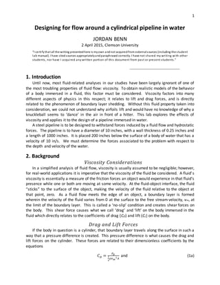
Figure 1. (a) Dye being released in a water tunnel to show the Karman Vortex
phenomenon. (b) The same apparatus ata slightly higher Reynolds number. The whorls
in the dye are created by the Karman vortices caused by the shedding boundary layer.
These vortices are called Karman vortices and are named as such for the man that first
described the phenomenon. The frequency at which the boundary layer sheds – and therefore,
at which these vortices are created – is governed by the equation
𝑓𝑠 =
𝑆𝑣∞
𝐷
, (2)
where S is the Strouhal number; a dimensionless variable that represents the ratio of local and
convective inertial forces. For the analysis in this lab, the Strouhal number was estimated to
have a value of 0.21.
The shedding frequency was experimentally checked against theoretical values using the
water tunnel in Figure 1. Red and blue dye were released from the top and bottom of a
cylindrical body immersed in the flow field of the water. The vortices were counted in pairs
over a time interval of 30 seconds for five different fluid velocities; this procedure was
performed three times at each fluid velocity and the results were averaged.
(a) (b)

3. 3
Figure 2. Theoretical and experimentally obtained Karman vortex shedding frequencies
at different fluid velocities. As can be seen, the experimental values are quite close to
the theoretical values calculated with Eq. 2.
Similarity Considerations
The basis for most fluid flow analysis relies on the dimensionless Reynolds number, Re. This
figure is based on the ratio of inertial and viscous forces experienced by a body immersed in a
flow. The equation for Re is,
𝑅𝑒 =
𝜌𝑣∞ 𝐷
𝜇
, (3)
where μ is the dynamic viscosity of the fluid and D is the diameter of the cylindrical (or
spherical) body in question.
Because this number is dimensionless, it can be used to relate the behavior of flows under
different conditions using a principle called similarity. This is a useful principle for modeling the
behavior of a fluid in a flow that is of a larger or smaller scale than is practical to test directly. If
a Reynolds number for a particular situation is obtained, then it can be concluded that as long
as the same Reynolds number is calculated for another situation, the flow will behave similarly.
3. Modeling Flow in a Wind Tunnel
To determine the parameters of the design problem given, a wind tunnel was used to
analyze the pressure variations on a cylinder caused by a fluid flow. The cylinder in the wind
tunnel had taps placed at 24 points around its circumference, from 0° to 180° (or 0 to π
radians). A pitot tube was used to indirectly measure the free stream velocity of the air by way
of the absolute pressure difference. This pressure difference is related to the free stream
velocity by the equation
∆𝑃 =
1
2
𝜌𝑣∞
2
. (4)
The coefficient of pressure (CP) is instrumental in obtaining the coefficient of drag on the
pipeline. The equation for CP is as follows:

4. Jordan Benn 4
𝐶 𝑃 =
𝑃𝑠−𝑃∞
1
2
𝜌𝑣∞
2
, (5)
where Ps is the pressure at that point on the surface of the cylinder and P∞ is the absolute
pressure in the environment. Using ideal conditions (assuming negligible viscosity) the
coefficient of pressure is calculated with the equation,
𝐶 𝑃 = 1 − 4(sin 𝜃)2
. (6)
The pressure difference was measured with a slant tube manometer in this case, using
water as the working fluid. Using Eq. 5 to obtain readings for CP, the following plots were
made:
Figure 3. Theoretical and experimentally obtained CP at (a) 8.27 in/s, (b) 33.86 in/s and
(c) 78.74 in/s. Evident in these plots is the separation point of the boundary layer. As
the experimental results depart from the theoretical model, so does the boundary layer
detach from the cylinder. Also, while the theoretical model shows symmetry across the
90° point, the experimental results do not show this; the pressure difference creates the
drag force.
The coefficient of drag can be calculated using the integral,
𝐶 𝐷 = ∫ 𝐶 𝑃( 𝜃) cos 𝜃 𝑑𝜃
𝜋
0
; (7)
however, this integral is fairly complicated to calculate directly. Using the trapezoid rule, this
integral can be approximated; the general equation for using the trapezoid rule is,
∫ 𝑓( 𝑥) 𝑑𝑥
𝑏
𝑎
= ∑
𝑓( 𝑥 𝑖)−𝑓( 𝑥 𝑖+1)
2
(𝑥 𝑖+1 − 𝑥 𝑖)𝑁
𝑖=1 , (8)
(a) (b)
(c)

5. 5
Using this approximation and Eq. 3, we can compare the drag coefficient to the Reynolds
number and obtain a relationship between the two quantities. This relationship and the
principle of similarity will aid in analyzing the forces acting on the designed pipeline. For the
situation described in the problem statement, Re = 72490.
Figure 4. Re versus CD for the three different velocities tested. The experimentally
obtained points of the plot are approximately linear, allowing the use of a linear
trendline in calculating the drag coefficient at the design point.
The above plot shows that the drag coefficient for the pipeline using the design parameters
laid out in the problem statement is, CD = 2.4306.
5. Pipeline Design
General Design
A free-body diagram (FBD) of the pipeline will aid in analyzing the forces on it and designing
a solution. This FBD is found below.
Figure 5. Free-body diagram of pipeline design.
Since the coefficient of drag is known, it is a fairly simple calculation to rearrange Eq. 1a to
obtain the drag force, FD. Once the drag force is found, we also know the force in the x-

6. Jordan Benn 6
direction that we must design for to resist the force of the flowing water; therefore, FD = Fx =
5248 lb. To obtain the normal force necessary in the y-direction, we just need to calculate the
weight of the pipe itself, and the water above it. For this we use the general equation for
weight W = ρ∙V, where V is the volume of the cylinder; this equation can also be used to find
the weight of the water above the cylinder. To this end, the weight of the water above the
cylinder and the cylinder itself sums to Wall = N = 74877 lb.
Uncertainty Considerations
The only measurable uncertainty associated with this design/analysis is the reading
obtained from the slant tube manometer. The pressure differences measured were recorded in
units of inches of water or, in-H2O. For the manometer, the resolution changed from one value
to another due to the construction of the manometer; below 2 in-H2O, the resolution was 0.01
in-H2O, however, above this reading, the resolution changed to 0.1 in-H2O. This makes the
zero-order uncertainty of the measurements uP = 0.005 in-H2O and 0.05 in-H2O, respectively.
When this situation occurs while obtaining data, it is best to take the largest resolution value
and over-estimate the uncertainty so as to not falsely skew the readings to make them finer
than they actually are.
In the scope of this analysis, the uncertainties associated with cases (a), (b) and (c)
propagate through to the final results in such a way that the uncertainty present in the final
results in negligible to the design. The pressure reading uncertainty associated with case (a) is
0.005 in-H2O, and the uncertainties associated with cases (b) and (c) are 0.05 in-H2O because of
the range of readings taken from the slant tube manometer.
6. Conclusion
Viscosity is too important a property to not be considered in real-world applications of
design associated with fluid flow. In fact, neglecting to include viscosity in this analysis and only
using the ideal equation for CP (Eq. 6) in the integral (Eq. 7) that calculates CD, results in a
coefficient of drag equal to zero; this in turn results in a pressure difference of zero. Having no
drag force in this situation would greatly simplify this design problem – since there would be no
drag force to design for – but would also cause the design to fail miserably if actually applied.

7. 7
REFERENCES
1. Figliola, R. S., and Donald E. Beasley. "5.6 Uncertainty Analysis: Error
Propagation." Theory and Design for Mechanical Measurements. Hoboken, NJ: J. Wiley,
2011. 261-66. Print.