Downloaded 19 times

![Simulation: a ubiquitous tool for statistical computation
Simulation, what’s that for?!
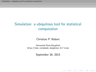
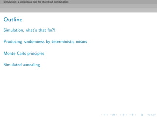
Illustrations
Necessity to “(re)produce chance” on a computer
Evaluation of the behaviour of a complex system (network,
computer program, queue, particle system, atmosphere,
epidemics, economic actions, &tc)
[ c Office of Oceanic and Atmospheric Research]](https://image.slidesharecdn.com/simulation-130926144124-phpapp01/85/Presentation-slides-for-my-simulation-course-at-Dauphine-6-320.jpg)
![Simulation: a ubiquitous tool for statistical computation
Simulation, what’s that for?!
Illustrations
Necessity to “(re)produce chance” on a computer
Production of changing landscapes, characters, behaviours in
computer games and flight simulators
[ c guides.ign.com]](https://image.slidesharecdn.com/simulation-130926144124-phpapp01/85/Presentation-slides-for-my-simulation-course-at-Dauphine-7-320.jpg)
![Simulation: a ubiquitous tool for statistical computation
Simulation, what’s that for?!
Illustrations
Necessity to “(re)produce chance” on a computer
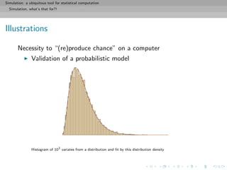
Determine probabilistic properties of a new statistical
procedure or under an unknown distribution [bootstrap]
(left) Estimation of the cdf F from a normal sample of 100 points;
(right) variation of this estimation over 200 normal samples](https://image.slidesharecdn.com/simulation-130926144124-phpapp01/85/Presentation-slides-for-my-simulation-course-at-Dauphine-8-320.jpg)
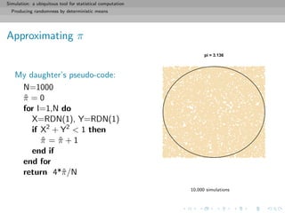
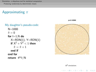
![Simulation: a ubiquitous tool for statistical computation
Simulation, what’s that for?!
Illustrations
Necessity to “(re)produce chance” on a computer
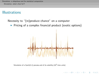
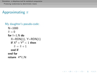
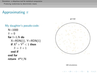
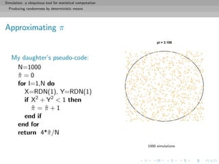
Approximation of a integral
[ c my daughter’s math book]](https://image.slidesharecdn.com/simulation-130926144124-phpapp01/85/Presentation-slides-for-my-simulation-course-at-Dauphine-10-320.jpg)
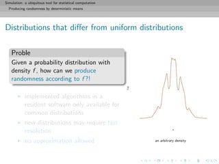
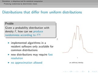
![Simulation: a ubiquitous tool for statistical computation
Simulation, what’s that for?!
Illustrations
Necessity to “(re)produce chance” on a computer
Maximisation of a weakly regular function/likelihood
[ c Dan Rice Sudoku blog]](https://image.slidesharecdn.com/simulation-130926144124-phpapp01/85/Presentation-slides-for-my-simulation-course-at-Dauphine-11-320.jpg)
![Simulation: a ubiquitous tool for statistical computation
Simulation, what’s that for?!
Illustrations
Necessity to “(re)produce chance” on a computer
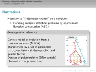
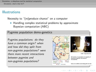
Handling complex statistical problems by approximate
Bayesian computation (ABC)
core principle
Simulate a parameter value (at random) and pseudo-data from the
likelihood until the pseudo-data is “close enough” to the observed
data, then
keep the corresponding parameter value
[Griffith & al., 1997; Tavar´e & al., 1999]](https://image.slidesharecdn.com/simulation-130926144124-phpapp01/85/Presentation-slides-for-my-simulation-course-at-Dauphine-13-320.jpg)
![Simulation: a ubiquitous tool for statistical computation
Producing randomness by deterministic means
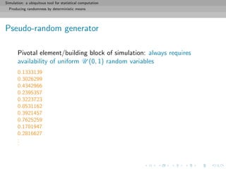
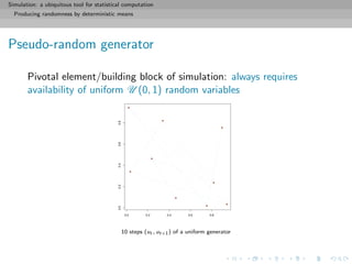
Pseudo-random generator
Pivotal element/building block of simulation: always requires
availability of uniform U (0, 1) random variables
[ c MMP World]](https://image.slidesharecdn.com/simulation-130926144124-phpapp01/85/Presentation-slides-for-my-simulation-course-at-Dauphine-16-320.jpg)
![Simulation: a ubiquitous tool for statistical computation
Producing randomness by deterministic means
Pseudo-random generator
Pivotal element/building block of simulation: always requires
availability of uniform U (0, 1) random variables
Definition (Pseudo-random generator)
A pseudo-random generator is a deterministic function f from ]0, 1[
to ]0, 1[ such that, for any starting value u0 and any n, the
sequence
{u0, f(u0), f(f(u0)), . . . , fn
(u0)}
behaves (statistically) like an iid U (0, 1) sequence](https://image.slidesharecdn.com/simulation-130926144124-phpapp01/85/Presentation-slides-for-my-simulation-course-at-Dauphine-18-320.jpg)

![Simulation: a ubiquitous tool for statistical computation
Producing randomness by deterministic means
A standard uniform generator
The congruencial generator on {1, 2, . . . , M}
f(x) = (ax + b) mod (M)
has a period equal to M for proper choices of (a, b) and becomes a
generator on ]0, 1[ when dividing by M + 1](https://image.slidesharecdn.com/simulation-130926144124-phpapp01/85/Presentation-slides-for-my-simulation-course-at-Dauphine-26-320.jpg)
![Simulation: a ubiquitous tool for statistical computation
Producing randomness by deterministic means
A standard uniform generator
The congruencial generator on {1, 2, . . . , M}
f(x) = (ax + b) mod (M)
has a period equal to M for proper choices of (a, b) and becomes a
generator on ]0, 1[ when dividing by M + 1
Example
Take
f(x) = (69069069x + 12345) mod (232
)
and produce
... 518974515 2498053016 1113825472 1109377984 ...
i.e.
... 0.1208332 0.5816233 0.2593327 0.2582972 ...](https://image.slidesharecdn.com/simulation-130926144124-phpapp01/85/Presentation-slides-for-my-simulation-course-at-Dauphine-27-320.jpg)
![Simulation: a ubiquitous tool for statistical computation
Producing randomness by deterministic means
A standard uniform generator
The congruencial generator on {1, 2, . . . , M}
f(x) = (ax + b) mod (M)
has a period equal to M for proper choices of (a, b) and becomes a
generator on ]0, 1[ when dividing by M + 1](https://image.slidesharecdn.com/simulation-130926144124-phpapp01/85/Presentation-slides-for-my-simulation-course-at-Dauphine-28-320.jpg)
![Simulation: a ubiquitous tool for statistical computation
Producing randomness by deterministic means
A standard uniform generator
The congruencial generator on {1, 2, . . . , M}
f(x) = (ax + b) mod (M)
has a period equal to M for proper choices of (a, b) and becomes a
generator on ]0, 1[ when dividing by M + 1](https://image.slidesharecdn.com/simulation-130926144124-phpapp01/85/Presentation-slides-for-my-simulation-course-at-Dauphine-29-320.jpg)
![Simulation: a ubiquitous tool for statistical computation
Producing randomness by deterministic means
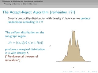
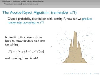
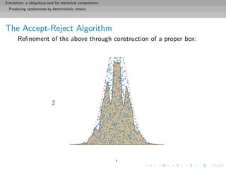
The Accept-Reject Algorithm
Refinement of the above through construction of a proper box:
1. Find a hat on f , i.e. a density g that can be simulated and
such that
sup
x
f (x) g(x) = M < ∞
2. Generate dots on the subgraph of g, i.e. Y1, Y2, . . . ∼ g, and
U1, U2, . . . ∼ U ([0, 1])
3. Accept only the Yk’s such that
Uk ≤ f (Yk)/Mg(Yk)](https://image.slidesharecdn.com/simulation-130926144124-phpapp01/85/Presentation-slides-for-my-simulation-course-at-Dauphine-39-320.jpg)
![Simulation: a ubiquitous tool for statistical computation
Producing randomness by deterministic means
The Accept-Reject Algorithm
Refinement of the above through construction of a proper box:
1. Find a hat on f , i.e. a density g that can be simulated and
such that
sup
x
f (x) g(x) = M < ∞
2. Generate dots on the subgraph of g, i.e. Y1, Y2, . . . ∼ g, and
U1, U2, . . . ∼ U ([0, 1])
3. Accept only the Yk’s such that
Uk ≤ f (Yk)/Mg(Yk)](https://image.slidesharecdn.com/simulation-130926144124-phpapp01/85/Presentation-slides-for-my-simulation-course-at-Dauphine-40-320.jpg)
![Simulation: a ubiquitous tool for statistical computation
Producing randomness by deterministic means
The Accept-Reject Algorithm
Refinement of the above through construction of a proper box:
1. Find a hat on f , i.e. a density g that can be simulated and
such that
sup
x
f (x) g(x) = M < ∞
2. Generate dots on the subgraph of g, i.e. Y1, Y2, . . . ∼ g, and
U1, U2, . . . ∼ U ([0, 1])
3. Accept only the Yk’s such that
Uk ≤ f (Yk)/Mg(Yk)](https://image.slidesharecdn.com/simulation-130926144124-phpapp01/85/Presentation-slides-for-my-simulation-course-at-Dauphine-41-320.jpg)

![Simulation: a ubiquitous tool for statistical computation
Producing randomness by deterministic means
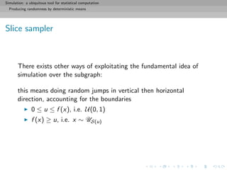
Slice sampler
There exists other ways of exploitating the fundamental idea of
simulation over the subgraph:
If direct uniform simulation on
Sf = {(u, x); 0 ≤ u ≤ f (x)}
is too complex [because of unavailable hat] use instead a random
walk on Sf :](https://image.slidesharecdn.com/simulation-130926144124-phpapp01/85/Presentation-slides-for-my-simulation-course-at-Dauphine-47-320.jpg)
![Simulation: a ubiquitous tool for statistical computation
Producing randomness by deterministic means
Slice sampler
Slice sampler algorithm
For t = 1, . . . , T
when at (x(t), ω(t)) simulate
1. ω(t+1) ∼ U[0,f (x(t))]
2. x(t+1) ∼ US(t+1) , where
S(t+1)
= {y; f (y) ≥ ω(t+1)
}.](https://image.slidesharecdn.com/simulation-130926144124-phpapp01/85/Presentation-slides-for-my-simulation-course-at-Dauphine-49-320.jpg)
![Simulation: a ubiquitous tool for statistical computation
Producing randomness by deterministic means
Slice sampler
Slice sampler algorithm
For t = 1, . . . , T
when at (x(t), ω(t)) simulate
1. ω(t+1) ∼ U[0,f (x(t))]
2. x(t+1) ∼ US(t+1) , where
S(t+1)
= {y; f (y) ≥ ω(t+1)
}.
0.0 0.2 0.4 0.6 0.8 1.0
0.0000.0020.0040.0060.0080.010
x
y](https://image.slidesharecdn.com/simulation-130926144124-phpapp01/85/Presentation-slides-for-my-simulation-course-at-Dauphine-50-320.jpg)
![Simulation: a ubiquitous tool for statistical computation
Producing randomness by deterministic means
Slice sampler
Slice sampler algorithm
For t = 1, . . . , T
when at (x(t), ω(t)) simulate
1. ω(t+1) ∼ U[0,f (x(t))]
2. x(t+1) ∼ US(t+1) , where
S(t+1)
= {y; f (y) ≥ ω(t+1)
}.
0.0 0.2 0.4 0.6 0.8 1.0
0.0000.0020.0040.0060.0080.010
x
y](https://image.slidesharecdn.com/simulation-130926144124-phpapp01/85/Presentation-slides-for-my-simulation-course-at-Dauphine-51-320.jpg)
![Simulation: a ubiquitous tool for statistical computation
Producing randomness by deterministic means
Slice sampler
Slice sampler algorithm
For t = 1, . . . , T
when at (x(t), ω(t)) simulate
1. ω(t+1) ∼ U[0,f (x(t))]
2. x(t+1) ∼ US(t+1) , where
S(t+1)
= {y; f (y) ≥ ω(t+1)
}.
0.0 0.2 0.4 0.6 0.8 1.0
0.0000.0020.0040.0060.0080.010
x
y](https://image.slidesharecdn.com/simulation-130926144124-phpapp01/85/Presentation-slides-for-my-simulation-course-at-Dauphine-52-320.jpg)
![Simulation: a ubiquitous tool for statistical computation
Producing randomness by deterministic means
Slice sampler
Slice sampler algorithm
For t = 1, . . . , T
when at (x(t), ω(t)) simulate
1. ω(t+1) ∼ U[0,f (x(t))]
2. x(t+1) ∼ US(t+1) , where
S(t+1)
= {y; f (y) ≥ ω(t+1)
}.
0.0 0.2 0.4 0.6 0.8 1.0
0.0000.0020.0040.0060.0080.010
x
y](https://image.slidesharecdn.com/simulation-130926144124-phpapp01/85/Presentation-slides-for-my-simulation-course-at-Dauphine-53-320.jpg)
![Simulation: a ubiquitous tool for statistical computation
Producing randomness by deterministic means
Slice sampler
Slice sampler algorithm
For t = 1, . . . , T
when at (x(t), ω(t)) simulate
1. ω(t+1) ∼ U[0,f (x(t))]
2. x(t+1) ∼ US(t+1) , where
S(t+1)
= {y; f (y) ≥ ω(t+1)
}.
0.0 0.2 0.4 0.6 0.8 1.0
0.0000.0020.0040.0060.0080.010
x
y](https://image.slidesharecdn.com/simulation-130926144124-phpapp01/85/Presentation-slides-for-my-simulation-course-at-Dauphine-54-320.jpg)
![Simulation: a ubiquitous tool for statistical computation
Producing randomness by deterministic means
Slice sampler
Slice sampler algorithm
For t = 1, . . . , T
when at (x(t), ω(t)) simulate
1. ω(t+1) ∼ U[0,f (x(t))]
2. x(t+1) ∼ US(t+1) , where
S(t+1)
= {y; f (y) ≥ ω(t+1)
}.
0.0 0.2 0.4 0.6 0.8 1.0
0.0000.0020.0040.0060.0080.010
x
y](https://image.slidesharecdn.com/simulation-130926144124-phpapp01/85/Presentation-slides-for-my-simulation-course-at-Dauphine-55-320.jpg)
![Simulation: a ubiquitous tool for statistical computation
Producing randomness by deterministic means
Slice sampler
Slice sampler algorithm
For t = 1, . . . , T
when at (x(t), ω(t)) simulate
1. ω(t+1) ∼ U[0,f (x(t))]
2. x(t+1) ∼ US(t+1) , where
S(t+1)
= {y; f (y) ≥ ω(t+1)
}.
0.0 0.2 0.4 0.6 0.8 1.0
0.0000.0020.0040.0060.0080.010
x
y](https://image.slidesharecdn.com/simulation-130926144124-phpapp01/85/Presentation-slides-for-my-simulation-course-at-Dauphine-56-320.jpg)
![Simulation: a ubiquitous tool for statistical computation
Producing randomness by deterministic means
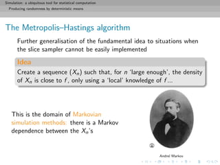
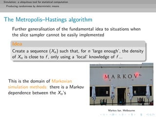
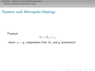
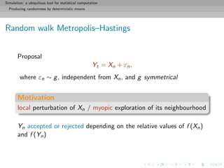
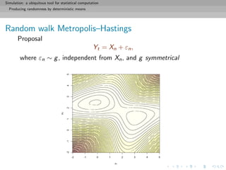
The Metropolis–Hastings algorithm
Further generalisation of the fundamental idea to situations when
the slice sampler cannot be easily implemented
‘local’ exploration can produce ‘global’ vision:
[ c Civilization 5]](https://image.slidesharecdn.com/simulation-130926144124-phpapp01/85/Presentation-slides-for-my-simulation-course-at-Dauphine-60-320.jpg)
![Simulation: a ubiquitous tool for statistical computation
Producing randomness by deterministic means
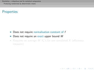
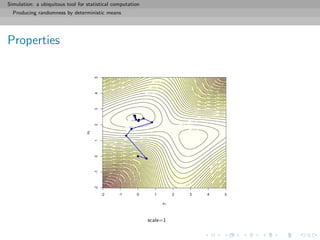
Properties
Always accepts higher point and sometimes lower points
(similar to gradient algorithms)
Depends on the dispersion of g
Average probability of acceptance
= min{f (x), f (y)}g(y − x) dxdy
close to 1 if g has a small variance [Danger!]
far from 1 if g has a large variance [Re-Danger!]](https://image.slidesharecdn.com/simulation-130926144124-phpapp01/85/Presentation-slides-for-my-simulation-course-at-Dauphine-67-320.jpg)
![Simulation: a ubiquitous tool for statistical computation
Producing randomness by deterministic means
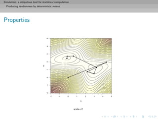
Properties
Always accepts higher point and sometimes lower points
(similar to gradient algorithms)
Depends on the dispersion of g
Average probability of acceptance
= min{f (x), f (y)}g(y − x) dxdy
close to 1 if g has a small variance [Danger!]
far from 1 if g has a large variance [Re-Danger!]](https://image.slidesharecdn.com/simulation-130926144124-phpapp01/85/Presentation-slides-for-my-simulation-course-at-Dauphine-68-320.jpg)
![Simulation: a ubiquitous tool for statistical computation
Producing randomness by deterministic means
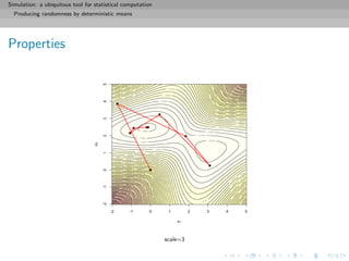
Properties
Always accepts higher point and sometimes lower points
(similar to gradient algorithms)
Depends on the dispersion of g
Average probability of acceptance
= min{f (x), f (y)}g(y − x) dxdy
close to 1 if g has a small variance [Danger!]
far from 1 if g has a large variance [Re-Danger!]](https://image.slidesharecdn.com/simulation-130926144124-phpapp01/85/Presentation-slides-for-my-simulation-course-at-Dauphine-69-320.jpg)
![Simulation: a ubiquitous tool for statistical computation
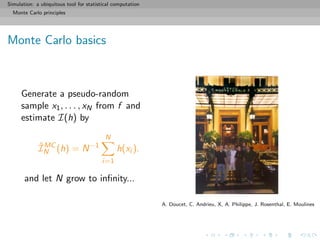
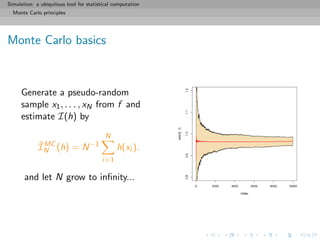
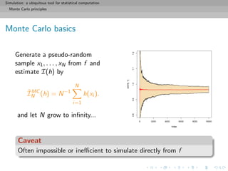
Monte Carlo principles
General purpose of Monte Carlo methods
Given a probability density f known up to a normalizing constant,
f (x) ∝ ˜f (x), and an integrable function h, compute
I(h) = h(x)f (x)dx =
h(x)˜f (x)dx
˜f (x)dx
when h(x)˜f (x)dx is intractable.
[Remember π!!]](https://image.slidesharecdn.com/simulation-130926144124-phpapp01/85/Presentation-slides-for-my-simulation-course-at-Dauphine-73-320.jpg)
![Simulation: a ubiquitous tool for statistical computation
Monte Carlo principles
General purpose of Monte Carlo methods
Given a probability density f known up to a normalizing constant,
f (x) ∝ ˜f (x), and an integrable function h, compute
I(h) = h(x)f (x)dx =
h(x)˜f (x)dx
˜f (x)dx
when h(x)˜f (x)dx is intractable.
[Remember π!!]](https://image.slidesharecdn.com/simulation-130926144124-phpapp01/85/Presentation-slides-for-my-simulation-course-at-Dauphine-74-320.jpg)
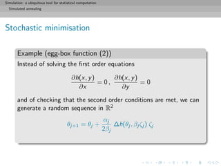
![Simulation: a ubiquitous tool for statistical computation
Simulated annealing
Optimisation problems
A (genuine) puzzle
During a dinner with 20 couples sitting at four tables with ten
seats, everyone wants to share a table with everyone. The
assembly decides to switch seats after each serving towards this
goal. What is the minimal number of servings needed to ensure
that every couple shared a table with every other couple at some
point? And what is the optimal switching strategy?
[http://xianblog.wordpress.com/2012/04/12/not-le-monde-puzzle/]
solution to the puzzle](https://image.slidesharecdn.com/simulation-130926144124-phpapp01/85/Presentation-slides-for-my-simulation-course-at-Dauphine-81-320.jpg)


![Simulation: a ubiquitous tool for statistical computation
Simulated annealing
Resolution via simulation
The simulated annealing algorithm:
name is borrowed from metallurgy
metal manufactured by a slow
decrease of temperature
(annealing) stronger than when
manufactured by fast decrease
[ c Joachim Robert, ca. 2006]](https://image.slidesharecdn.com/simulation-130926144124-phpapp01/85/Presentation-slides-for-my-simulation-course-at-Dauphine-94-320.jpg)
![Simulation: a ubiquitous tool for statistical computation
Simulated annealing
Resolution via simulation
Repeat
Random modifications of parts of the original circuit with cost
C0
Evaluation of the cost C of the new circuit
Acceptation of the new circuit with probability
min exp
C0 − C
T
, 1
[Metropolis et al., 1953]](https://image.slidesharecdn.com/simulation-130926144124-phpapp01/85/Presentation-slides-for-my-simulation-course-at-Dauphine-95-320.jpg)
![Simulation: a ubiquitous tool for statistical computation
Simulated annealing
Resolution via simulation
Repeat
Random modifications of parts of the original circuit with cost
C0
Evaluation of the cost C of the new circuit
Acceptation of the new circuit with probability
min exp
C0 − C
T
, 1
T, temperature, is progressively reduced
[Metropolis et al., 1953]](https://image.slidesharecdn.com/simulation-130926144124-phpapp01/85/Presentation-slides-for-my-simulation-course-at-Dauphine-96-320.jpg)
![Simulation: a ubiquitous tool for statistical computation
Simulated annealing
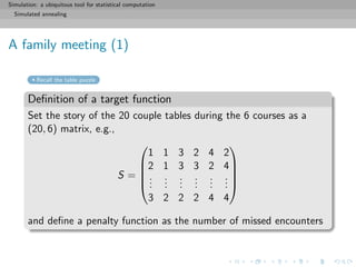
A family meeting (1)
Recall the table puzzle
Definition of a target function
I=sample(rep(1:4,5))
for (i in 2:6)
I=cbind(I,sample(rep(1:4,5)))
meet=function(I){
M=outer(I[,1],I[,1],"==")
for (i in 2:6)
M=M+outer(I[,i],I[,i],"==")
M
}
penalty=function(M){ sum(M==0) }
penat=penalty(meet(I))](https://image.slidesharecdn.com/simulation-130926144124-phpapp01/85/Presentation-slides-for-my-simulation-course-at-Dauphine-98-320.jpg)
![Simulation: a ubiquitous tool for statistical computation
Simulated annealing
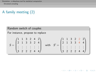
A family meeting (2)
Random switch of couples
Pick two couples [among the 20 couples] at random with
probabilities proportional to the number of other couples they
have not seen
prob=apply(meet(I)==0,1,sum)
switch their respective position during one of the 6 courses
accept the switch with Metropolis–Hastings probability
log(runif(1))<(penalty(old)-penalty(new))/gamma](https://image.slidesharecdn.com/simulation-130926144124-phpapp01/85/Presentation-slides-for-my-simulation-course-at-Dauphine-99-320.jpg)
![Simulation: a ubiquitous tool for statistical computation
Simulated annealing
A family meeting (2)
Random switch of couples
for (t in 1:N){
prop=sample(1:20,2,prob=apply(meet(I)==0,1,sum))
cour=sample(1:6,1)
Ip=I
Ip[prop[1],cour]=I[prop[2],cour]
Ip[prop[2],cour]=I[prop[1],cour]
penatp=penalty(meet(Ip))
if (log(runif(1))<(penat-penatp)/gamma){
I=Ip
penat=penatp}
}](https://image.slidesharecdn.com/simulation-130926144124-phpapp01/85/Presentation-slides-for-my-simulation-course-at-Dauphine-101-320.jpg)
![Simulation: a ubiquitous tool for statistical computation
Simulated annealing
A family meeting (3)
Solution
I
[1,] 1 4 3 2 2 3
[2,] 1 2 4 3 4 4
[3,] 3 2 1 4 1 3
[4,] 1 2 3 1 1 1
[5,] 4 2 4 2 3 3
[6,] 2 4 1 2 4 1
[7,] 4 3 1 1 2 4
[8,] 1 3 2 4 3 1
[9,] 3 3 3 3 4 3
[10,] 4 4 2 3 1 1
[11,] 1 1 1 3 3 2
[12,] 3 4 4 1 3 2
[13,] 4 1 3 4 4 2
[14,] 2 4 3 4 3 4
[15,] 2 3 4 2 1 2
[16,] 2 2 2 3 2 2
[17,] 2 1 2 1 4 3
[18,] 4 3 1 1 2 4
[19,] 3 1 4 4 2 1
[20,] 3 1 2 2 1 4 [ c http://www.metrolyrics.com]](https://image.slidesharecdn.com/simulation-130926144124-phpapp01/85/Presentation-slides-for-my-simulation-course-at-Dauphine-102-320.jpg)
![Simulation: a ubiquitous tool for statistical computation
Simulated annealing
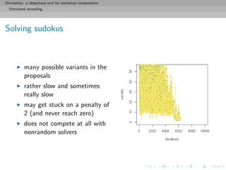
Solving sudokus
Solving a Sudoku grid as a minimisation problem:
[ c Dan Rice Sudoku blog]](https://image.slidesharecdn.com/simulation-130926144124-phpapp01/85/Presentation-slides-for-my-simulation-course-at-Dauphine-103-320.jpg)
![Simulation: a ubiquitous tool for statistical computation
Simulated annealing
Solving sudokus
Given a partly filled Sudoku grid (with a single solution),
define a random Sudoku grid by filling the empty slots at
random
s=matrix(0,ncol=9,nrow=9)
s[1,c(1,6,7)]=c(8,1,2)
s[2,c(2:3)]=c(7,5)
s[3,c(5,8,9)]=c(5,6,4)
s[4,c(3,9)]=c(7,6)
s[5,c(1,4)]=c(9,7)
s[6,c(1,2,6,8,9)]=c(5,2,9,4,7)
s[7,c(1:3)]=c(2,3,1)
s[8,c(3,5,7,9)]=c(6,2,1,9)](https://image.slidesharecdn.com/simulation-130926144124-phpapp01/85/Presentation-slides-for-my-simulation-course-at-Dauphine-104-320.jpg)
![Simulation: a ubiquitous tool for statistical computation
Simulated annealing
Solving sudokus
Given a partly filled Sudoku grid (with a single solution),
define a random Sudoku grid by filling the empty slots at
random
define a penalty function corresponding to the number of
missed constraints
#local score
scor=function(i,s){
a=((i-1)%%9)+1
b=trunc((i-1)/9)
boxa=3*trunc((a-1)/3)+1
boxb=3*trunc(b/3)+1
return(sum(s[i]==s[9*b+(1:9)])+
sum(s[i]==s[a+9*(0:8)])+
sum(s[i]==s[boxa:(boxa+2),boxb:(boxb+2)])-3)
}](https://image.slidesharecdn.com/simulation-130926144124-phpapp01/85/Presentation-slides-for-my-simulation-course-at-Dauphine-105-320.jpg)
![Simulation: a ubiquitous tool for statistical computation
Simulated annealing
Solving sudokus
Given a partly filled Sudoku grid (with a single solution),
define a random Sudoku grid by filling the empty slots at
random
define a penalty function corresponding to the number of
missed constraints
fill “deterministic” slots
make simulated annealing moves
# random moves on the sites
i=sample((1:81)[as.vector(s)==0],sample(1:sum(s==0),1,pro=1/(1:sum(s==0))))
for (r in 1:length(i))
prop[i[r]]=sample((1:9)[pool[i[r]+81*(0:8)]],1)
if (log(runif(1))/lcur<tarcur-target(prop)){
nchange=nchange+(tarcur>target(prop))
cur=prop
points(t,tarcur,col="forestgreen",cex=.3,pch=19)
tarcur=target(cur)
}](https://image.slidesharecdn.com/simulation-130926144124-phpapp01/85/Presentation-slides-for-my-simulation-course-at-Dauphine-106-320.jpg)

The document discusses the role of simulation as a fundamental tool in statistical computation, particularly focusing on Monte Carlo methods and the bootstrap technique. It highlights the practical applications of simulation in various fields such as finance, epidemiology, and computer gaming, emphasizing the importance of producing randomness deterministically through pseudo-random generators. The content includes references and resources to enhance understanding and skill development in using R programming for simulations.