This document describes a study that investigated the spatial scale of variability in normalized surface wave heights in a near-shore coastal environment. Two wave buoys equipped with inertial motion sensors were designed and deployed at varying distances apart along a 400m stretch of beach. Wave data was collected and analyzed to determine the spatial scale at which wave heights became dissimilar between sensor locations, indicating separate controlling processes. Preliminary results from a 16.89m deployment suggested non-stationary wave processes operating at multiple spatial scales over hundreds of meters. Further analysis of the full dataset aimed to better understand wave behaviors and inform optimal siting of wave energy converters.


![22 | S e t i a w a n
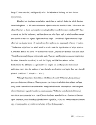
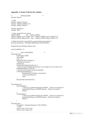
Appendix C. MATLAB Scripts for calculations and graphing
I. waveCalc.m
%This is the code for the raw calculations Function
function [position,tMod,avgperiod,sigwaveheight,power] = waveCalc(wave,fileName,...
ax,ay,az,gx,gy,gz,t)
%% Import data
rawdata = importdata(fileName);
IMUdata = rawdata;
samplePeriod = 1/2;
acc = [IMUdata(:,ax),IMUdata(:,ay),IMUdata(:,az)]; % accelerometer
gyr = [IMUdata(:,gx),IMUdata(:,gy),IMUdata(:,gz)];
time = IMUdata(:,t);
% time is changed to start from 0
tMod = zeros(length(time),1);
for kk = 1:length(time)-1
tMod = time - time(1,1);
end
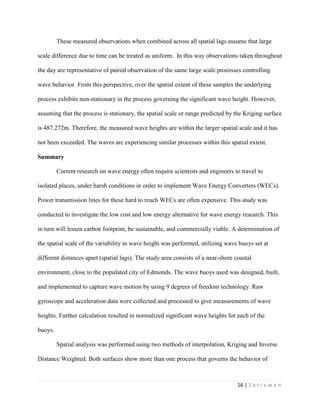
%% Calculations
% calculate orientation
R = zeros(3,3,length(gyr)); % rotation matrix describing sensor relative to Earth
for i = 1:length(gyr)
R(1,1,i) = cos(gyr(i,3)).*cos(gyr(i,2));
R(1,2,i) = (cos(gyr(i,3)).*sin(gyr(i,2)).*sin(gyr(i,1)))-(sin(gyr(i,3)).*cos(gyr(i,1)));
R(1,3,i) = (cos(gyr(i,3)).*sin(gyr(i,2)).*cos(gyr(i,1)))+(sin(gyr(i,3)).*sin(gyr(i,1)));
R(2,1,i) = sin(gyr(i,3)).*cos(gyr(i,2));
R(2,2,i) = (sin(gyr(i,3)).*sin(gyr(i,2)).*sin(gyr(i,1)))+(cos(gyr(i,3)).*cos(gyr(i,1)));
R(2,3,i) = (sin(gyr(i,3)).*sin(gyr(i,2)).*cos(gyr(i,1)))-(cos(gyr(i,3)).*sin(gyr(i,1)));
R(3,1,i) = -sin(gyr(i,2));
R(3,2,i) = cos(gyr(i,2)).*sin(gyr(i,1));
R(3,3,i) = cos(gyr(i,2)).*cos(gyr(i,1));
end
% Calculate 'tilt-compensated' accelerometer
tcAcc = zeros(size(acc)); % accelerometer in Earth frame
for i = 1:length(acc)
tcAcc(i,:) = R(:,:,i) * acc(i,:)';
end
% Calculate linear acceleration in Earth frame (subtracting gravity)
linAcc = tcAcc - [zeros(length(tcAcc), 1), zeros(length(tcAcc), 1), ones(length(tcAcc), 1)];
% Calculate linear velocity (integrate acceleration)
linVel = zeros(size(linAcc));
for i = 2:length(linAcc)
linVel(i,:) = linVel(i-1,:) + linAcc(i,:) * samplePeriod;
end
% High-pass filter linear velocity to remove drift
order = 1;
filtCutOff = 0.1;](https://image.slidesharecdn.com/8d655b56-f6c3-4ae8-b20b-9614dcc8e582-150604021925-lva1-app6891/85/Setiawan_Landung_Final_Senior_Thesis-23-320.jpg)
![23 | S e t i a w a n
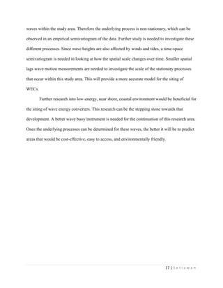
[b, a] = butter(order, (2*filtCutOff)/(1/samplePeriod), 'high');
linVelHP = filtfilt(b, a, linVel);
% Calculate linear position (integrate velocity)
linPos = zeros(size(linVelHP));
for i = 2:length(linVelHP)
linPos(i,:) = linPos(i-1,:) + linVelHP(i,:) * samplePeriod;
end
% High-pass filter linear position to remove drift
order = 1;
filtCutOff = 0.1;
[b, a] = butter(order, (2*filtCutOff)/(1/samplePeriod), 'high');
linPosHP = filtfilt(b, a, linPos);
position = (linPosHP .* 0.40);
% Calculate Height and Avg. Height
height = zeros(length(position(:,3)),1);
for zz = 1:length(position(:,3)) - 1
if linPosHP(zz,3) > 0
height(zz,:) = linPosHP(zz,3);
end
end
averageHeight = sum(height)/length(height);
%wave period calculation
buoyOne = [tMod,height];
remZero = buoyOne(:,2)==0;
buoyOne(remZero,:) = [];
% calculating change in time at every time step
period = zeros(length(buoyOne(:,1)),1);
for jj = 1:length(buoyOne(:,1))-1
period(jj,1) = buoyOne(jj+1,1) - buoyOne(jj,1);
end
% calculate average period
avgperiod = mean(period);
% significant wave height
sigwaveheight = 4 * sqrt(var(position(:,3)));
% power kW/m
power = 0.57 * (sigwaveheight^2) * avgperiod;
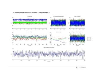
%% Senior Thesis Graph
figure('Name', strcat(fileName,wave));
%raw accelerometer
subplot(3,4,[1 2]);
hold on;
plot(tMod,acc(:,1), 'r');
plot(tMod,acc(:,2), 'g');
plot(tMod,acc(:,3), 'b');
axis([0 900 -20 20]);
ylabel('m/s^2');
title('Accelerometer');
legend1 = legend('X', 'Y', 'Z');
set(legend1,'Position',[0.929233772571985 0.467726396917148 0.0490483162518301 0.0876685934489403]);](https://image.slidesharecdn.com/8d655b56-f6c3-4ae8-b20b-9614dcc8e582-150604021925-lva1-app6891/85/Setiawan_Landung_Final_Senior_Thesis-24-320.jpg)
![24 | S e t i a w a n
%tilt compesated accelerometer
subplot(3,4,3);
hold on;
plot(tMod,tcAcc(:,1), 'r');
plot(tMod,tcAcc(:,2), 'g');
plot(tMod,tcAcc(:,3), 'b');
axis([0 900 -20 20]);
ylabel('m/s^2');
title('''Tilt-compensated'' accelerometer');
%linear acceleration
subplot(3,4,4);
hold on;
plot(tMod,linAcc(:,1), 'r');
plot(tMod,linAcc(:,2), 'g');
plot(tMod,linAcc(:,3), 'b');
axis([0 900 -20 20]);
ylabel('m/s^2');
title('Linear acceleration');
%linear velocity
subplot(3,4,7);
hold on;
plot(tMod,linVel(:,1), 'r');
plot(tMod,linVel(:,2), 'g');
plot(tMod,linVel(:,3), 'b');
axis([0 900 -800 800]);
xlabel('seconds');
ylabel('m/s');
title('Linear velocity');
%High-pass linear velocity
subplot(3,4,8);
hold on;
plot(tMod,linVelHP(:,1), 'r');
plot(tMod,linVelHP(:,2), 'g');
plot(tMod,linVelHP(:,3), 'b');
axis([0 900 -10 10]);
xlabel('seconds');
ylabel('m/s');
title('High-pass filtered linear velocity');
%linear position
subplot(3,4,[5 6]);
hold on;
plot(tMod,linPos(:,1), 'r');
plot(tMod,linPos(:,2), 'g');
plot(tMod,linPos(:,3), 'b');
axis([0 900 -30 30]);
xlabel('seconds');
ylabel('m');
title('Linear position');
%high-filtered position
subplot(3,4,[9 10 11 12]);
hold on;
plot(tMod,position(:,3), 'b');
axis([0 900 -2 2]);
xlabel('seconds');
ylabel('m');
title('High-pass filtered linear position');](https://image.slidesharecdn.com/8d655b56-f6c3-4ae8-b20b-9614dcc8e582-150604021925-lva1-app6891/85/Setiawan_Landung_Final_Senior_Thesis-25-320.jpg)
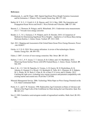
![25 | S e t i a w a n
hold off;
end
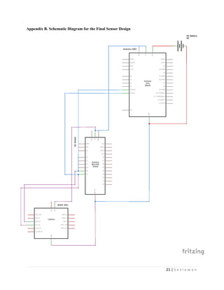
II. waveProcess.m
%The function that takes in the raw data, calling waveCalc function and gives out data array Results
function [Results] = waveProcess(file)
[position1, tMod1, avgPeriod1, sigwaveheight1, power1] = ...
waveCalc('_wave_1',file,6,7,8,3,4,5,1);
[position2, tMod2, avgPeriod2, sigwaveheight2, power2] = ...
waveCalc('_wave_2',file,14,15,16,11,12,13,9);
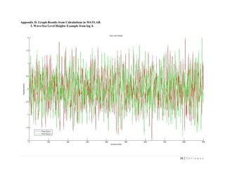
figure('Name', strcat(file,'_Position Data'));
hold on;
plot(tMod1,position1(:,1), 'r');
plot(tMod2,position2(:,2), 'g');
axis([0 900 -2 2]);
xlabel('time(seconds)');
ylabel('height(meters)');
title('High-pass filtered linear position');
legend1 = legend('Wave Buoy I', 'Wave Buoy II');
set(legend1,'Position',[0.143728648121013 ...
0.142100192678225 0.0980966325036558 0.0606936416184971]);
Results = dataset({sigwaveheight1,'Significant Wave HeightI'},...
{avgPeriod1,'Wave PeriodI'},...
{power1,'PowerI'},...
{sigwaveheight2,'Significant Wave HeightII'},...
{avgPeriod2,'Wave PeriodII'},...
{power2,'PowerII'});
End
III. Results.m
%This script exports the resulting data arrays to excel files
clear all; close all; clc
[resultLag1] = waveProcess('lag_1.csv');
export(resultLag1,'XLSFile','lag_1Results.xlsx')
[resultLag2] = waveProcess('lag_2.csv');
export(resultLag2,'XLSFile','lag_2Results.xlsx')
[resultLag3] = waveProcess('lag_3.csv');
export(resultLag3,'XLSFile','lag_3Results.xlsx')
[resultLag4] = waveProcess('lag_4.csv');
export(resultLag4,'XLSFile','lag_4Results.xlsx')
[resultLag5] = waveProcess('lag_5.csv');
export(resultLag5,'XLSFile','lag_5Results.xlsx')
[resultLag6] = waveProcess('lag_6.csv');
export(resultLag6,'XLSFile','lag_6Results.xlsx')
[resultLag7] = waveProcess('lag_7.csv');
export(resultLag7,'XLSFile','lag_7Results.xlsx')](https://image.slidesharecdn.com/8d655b56-f6c3-4ae8-b20b-9614dcc8e582-150604021925-lva1-app6891/85/Setiawan_Landung_Final_Senior_Thesis-26-320.jpg)