This document discusses an experiment analyzing wave loadings on a Seawave Slot-cone Generator (SSG), a wave energy converter. Regular wave tests were conducted in a wave flume on a 1:66 scale model of the SSG located on a sloped "focuser" to increase wave run-up. Pressure transducers measured wave pressures at different heights on the SSG during 31 wave trains with varying heights and periods. The results were used to develop predictive methods for estimating peak wave pressures and rise times on the SSG under different conditions. These predictions will help with structural design of full-scale SSG devices.

1. Nature and magnitude of wave loadings at Seawave
Slot-cone Generators
M. Buccino a
, D. Vicinanza b,n
, B. Mohammadi
c
, D. Ban d
, M. Calabrese
a
a
Department of Civil, Architectural and Environmental Engineering, University of Naples, Federico II Via Claudio 21, 80125 Napoli, Italy
b
Department of Civil Engineering, Design, Building and Environment (DICDEA), Seconda Università di Napoli (SUN), Via Roma 29, 81031 Aversa (CE), Italy
c
Department of Maritime Civil Engineering-Offshore Engineering, Science and Branch, Islamic Azad University, Tehran, Iran
d
School of Marine Science and Engineering, Plymouth University Drake Circus, Plymouth PL48AA, UK
a r t i c l e i n f o
Article history:
Received 13 May 2014
Accepted 30 November 2014
Available online 25 December 2014
Keywords:
Wave energy converters
Wave breaking
Wave loadings
Laboratory experiments
Scale effects
a b s t r a c t
The Seawave Slot-cone Generator (SSG) is a wave energy converter based on the overtopping principle,
which has collected a good deal of funds in the last years, from both public and private investors.
Although its functional response has been extensively researched, practically no tools exist for the
structural design. Based on the results of regular wave experiments conducted at the University of
Naples Federico II (Italy), a number of design equations have been derived, which permit to estimate the
magnitude of the wave pressures acting onto the outer face of the device, along with the respective rise
times. The reliability of the predictive methods have been then verified against the random wave
experiments of Vicinanza and Frigaard (2009).
& 2014 Published by Elsevier Ltd.
1. Introduction
The high concentration of greenhouse gases in the atmosphere,
about 400 ppm, makes the de-carbonization of the energy sector a
binding need for the whole planet. For this reason clean energy
investment is continuously increasing even in economically chal-
lenging times and has reached the amount of $ 244 billion in 2012
(REN21 Global Status Report, 2013).
The wave energy has the potential to be a particularly valuable
contributor to a low-carbon energy mix, since, beside being very
abundant (Brooke, 2003; Clement et al., 2002; Falnes, 2002), it has
a different geographic distribution than wind and solar, greater
predictability and less intermittency. Accordingly, even in the
awareness that only a small fraction of this huge resource can be
exploited, more than 1000 Wave Energy Converters (WECs) have
been patented worldwide.
However, a number of prototype generators were destroyed in
storms (Falcão, 2010), making evident that the lack of a specific
knowledge on the capability of WECs of resisting wave actions
may represent a serious hurdle, of both technical and economical
nature, to the development of the devices.
Bearing this in mind, the Danish Council for Strategic Research
has recently supported the project Structural Design of Wave
Energy Devices (SDWED; Kofoed et al., 2010), whereas the Eur-
opean Commission has funded the GEOwave consortium (http://
www.geowave-r4sme.eu), which brings together universities and
private companies with the purpose of conducting industry
specified research on anchoring and mooring systems expressly
designed for WECs. Furthermore, in the development of an
“integrated” overtopping-type WEC which uses a reservoir incor-
porated in a common rubble mound breakwater, Vicinanza et al.
(2014) analyzed with much attention the nature of wave loadings
acting on the tank, providing accurate methods for their
prediction.
In this paper, the case of the Seawave Slot-cone Generator
(SSG) is tackled. Patented by WavEnergy SAS (Stavanger, Norway),
this device includes a number of reservoirs placed on the top of
each-other, which capture the water during the up-rush phase
(Fig. 1); on its way back to the sea, the fluid passes through a low
head turbine, spinning it and producing electricity.
The WEC is normally located at the top of a steep foreshore,
which has the purpose of increasing the potential run-up height;
the latter will be nicknamed “focuser” in the following, as a
reworked version of the term “concentrator” introduced by
Polinder and Scuotto (2005) in describing the general functioning
of the converters based on the overtopping principle.
The SSG technology has collected a good deal of funds in the
last years and two pilot plants were planned to be located along
Contents lists available at ScienceDirect
journal homepage: www.elsevier.com/locate/oceaneng
Ocean Engineering
http://dx.doi.org/10.1016/j.oceaneng.2014.11.038
0029-8018/& 2014 Published by Elsevier Ltd.
n
Corresponding author.
E-mail addresses: buccino@unina.it (M. Buccino),
diego.vicinanza@unina2.it (D. Vicinanza), b.mohammadi@srbiau.ac.ir (B. Mohammadi),
davide.banfi@plymouth.ac.uk (D. Banfi), calabres@unina.it (M. Calabrese).
Ocean Engineering 95 (2015) 34–58

2. the West Norwegian coasts; one at the isle of Kvitsøy (in the Bokna
fjord), the other around Svåheia (Fig. 2).
The extensive investigations carried out on the hydraulic
performances of the device (Margheritini et al. 2009; Vicinanza
et al., 2012), allowed deriving a number of equations where the
amount of water entering the reservoirs can be reliably estimated
under different wave conditions, including oblique and short-
crested seas. Conversely, practically no tools exist for the structural
design.
In this respect, the wider experimental study available to date
is that of Vicinanza and Frigaard (2009), which though could not
lead to any general conclusion, since the tests reproduced the
specific climate of the site of Kvitsøy. Successive investigations
conducted during the design of the Svåheia plant (e.g. Buccino
et al., 2011) encompassed a very narrow set of data, with a limited
variance of the hydraulic parameters.
Therefore, to fill the gap new experiments have been per-
formed at the University of Naples Federico II (Italy). Here, the
wave parameters have been varied enough to get a wide spectrum
of loading cases. Moreover, it has been chosen to work with
regular waves to study the structure response under very simple
forcings. From the analysis of data a set of design tools have been
derived, the reliability of which have been then checked against
the random wave experiments of Vicinanza and Frigaard (2009).
The article is organized as follows. After a description of the
experimental set-up (Section 2), the Sections 3 and 4 discuss the
qualitative features of the observed wave profiles and of the
actions they induce on the SSG. In Section 5, a preliminary map
for the prediction of the different loading cases is presented. A
probabilistic design tool for the estimation of the peak pressures
acting on the front face of the wall is given in Section 6. The
predictive method is finally compared to random wave data in
Section 7.
2. Experimental work
2.1. Facility and model
The experiments have been carried out at the Small Scale
Channel (SSC) of the Laboratorio di Ingegneria Costiera (LInC) of
the Department of Civil, Architectural and Environmental Engi-
neering (DICEA) of the University of Naples Federico II. The flume,
22 m long, 0.5 m wide and 0.75 m deep, is equipped with a piston-
type wavemaker capable of generating both periodic and random
wave series. The facility is also provided with an active absorption
system, to dampen any undesired reflection generated by the
structures installed within it.
The SSG was a 1:66 scale model of the Svåheia pilot plant
(Fig. 3); it was made of plexiglass, with the front plates inclined by
351 to the horizontal.
Nomenclature
Bgn Bagnold number
Csample correction coefficient of pressures and forces consid-
ering the sampling effect
Cscale correction coefficient of pressures and forces consid-
ering the scale effect
D mean thickness of the air pocket
d water level in the channel
E expectation operator
^F1=250 mean of the highest 1/250th peaks of force
Fint integrated wave force
g gravity acceleration
h water depth at the toe of SSG
hc wall height
H wave height
H1/3 significant wave height
Hm0 significant (spectral) wave height
H/L wave steepness
KW thickness of water mass effectively contributing to
the impact
KR reflection coefficient
k wave number
kd relative water depth
L wave length
LTP Linear Thrust Parameter
m correction coefficient for ^pav
MF wave momentum flux through the base of the focuser
MFP Momentum Flux Parameter
p0 atmospheric pressure
^p pressure peak
^pav average pressure
^pmax maximum pressure
r correlation coefficient
Rc crest freeboard of SSG
se standard error
S mean slope parameter
S0 still water thrust at the base of the focuser
tr peak rise time
tgαav average value of the slope
T wave period
T1/3 significant wave period
Tp peak wave period
u cross-shore wave velocity
u0 velocity of the water hammer
X vector of the log-variables
z vertical coordinate
ZG vertical distance of pressure barycentre from the
structure toe
η free surface
λF Froude scale factor
λS scale correction factor
μ vector of averages of the log-variables
Πx horizontal component of the peak force exerted on the
structure
ξ inshore Iribarren number
ρ water density
Σ matrix of covariance
Fig. 1. Artistic representation of a 3-level SSG.
M. Buccino et al. / Ocean Engineering 95 (2015) 34–58 35

3. Along with the WEC, also the steeper part of the foreshore (the
“focuser”) has been reproduced at the same scale (Fig. 4). The beach
extended about 1.39 m towards the wavemaker and included a 1:5
approaching slope followed by two ramps with an inclination of
respectively 1:1 and 1:2.5. Between the toe of the approaching
slope and the wavemaker, the bottom of the flume was flat.
The SSG has been seated on a horizontal strip of plexiglass
extending about 1 m beyond its heel.
All tests were conducted with a water level in the channel,
d¼0.50 m; accordingly, the WEC had the crest freeboard (Rc)
0.10 m above the swl, whereas the water depth at its toe, h, was
0.056 m.
Fig. 2. The sites of Kvitsøy (left panel) and Svåheia (right panel).
Fig. 3. Sketch of the SSG model. Dimensions in mm.
h = 0.056
0.500
1
2.5
1
1
1
5
S.W.L
1.3861.008 0.361
2.755
Fig. 4. The bathymetry and the location of the WEC. Dimensions in m (model scale).
M. Buccino et al. / Ocean Engineering 95 (2015) 34–5836

4. 2.2. Waves
Thirty-one regular wave trains with a duration of 128 s have
been run, divided into four subsets of constant period, T. The
values of the latter (0.8 s, 1.0 s, 1.5 s, 2.0 s) were chosen in order to
get a range of relative water depths, kd, spanning from deep
waters (4π) to quasi-shallow waters (o1).
The incident wave heights at the toe of the “focuser” were
varied between 2.6 cm and 22 cm; this gave values of the wave
steepness ranging from 0.006 to 0.124. No waves have been
observed to break seawards the approaching slope.
2.3. Control of water level behind the device
During the tests, the water passing over the roof of the SSG was
conveyed back to the wave-maker via a submersible pump with a
maximum capacity of 375 l/min (Fig. 5). The pump was lodged in a
0.147 m3
reservoir built about 4 m off the trailing edge of the
structure. A valve permitted to control the amount of discharge.
A porous mound, made of cobblestone, has been placed
between the model and the reservoir to absorb the waves
generated by overtopping in the sheltered area.
2.4. Measurements
Four twin-wire resistive probes sampled at 25 Hz were placed
seaward the “focuser” to separate incident and reflected waves
through the method of Zelt and Skjelbreia (1992), which is based
on a weighted least square approach. The separation procedure
has been applied to the band 0.5–1.5 the fundamental wave
frequency. For the analysis to be as reliable as possible, the probes
position has been optimized test by test using the frequency
response function suggested by Zelt and Skjelbreia at the Eq. (20)
of their paper.
0.40m0.12m2.25m
Absorbing moundEnd of the channel
Reservoir
Plastic pipe
2cm2cm
Valve
To the rear of the wavemaker
Wave probe
Fig. 5. View of the recirculation system. Top panels: reservoir (left) with pump and plastic pipe at the rear of the wavemaker (right). Low panel: general sketch of the system.
Fig. 6. Position and features of the pressure transducers.
M. Buccino et al. / Ocean Engineering 95 (2015) 34–58 37

5. As shown in the low panel of Fig. 5, an additional wave gauge
was used to check the water level in the reservoir during the
pumping process.
Four piezo-resistive pressure transducers with a cut-off fre-
quency of 20 kHz were positioned along the outer plates of the
SSG, according to the scheme of Fig. 6 (see also Table 2). The
sensors had a diameter of 18 mm and were sampled at 1 kHz.
The center of the transducer “p1” was 1.40 cm above the toe of
the wall, whilst “p2” recorded the pressure signal at the swl. “p3”
and “p4” were located in the middle of the second and third plate
respectively, where Vicinanza and Frigaard (2009) measured the
maximum values of loadings. The center of the transducer “p4”
was 2.35 cm below the top of the WEC.
A digital video camera was employed to record the macroscopic
features of the wave profiles.
2.5. Data processing
From the application of the Zelt and Skjelbreia method, the
time-domain fluctuations of the incident and the reflected wave
profiles were obtained. As mentioned before, these signals were
limited in the band 0.5–1.5 the fundamental frequency of the
waves. The chronograms were subjected to zero up crossing and
for each of them the wave height and period have been con-
ventionally assimilated to the mean of the highest third of the
waves (H1/3 and T1/3). This is consistent with the suggestions of
Goda (1986).
Dividing the reflected wave height by the incident one, the
reflection coefficient KR has been obtained, which obviously refers
to the whole model including the foreshore and the SSG.
As far as the pressure data is concerned, the following quan-
tities have been calculated for each wave period and each
transducer:
the pressure peak ^p, i.e. the maximum pressure over a
wave cycle;
the peak rise time tr, i.e. the time interval between the pressure
levels corresponding to the 2.5% and the 97.5% of the peak
value ^p. Note that for a simple sine wave, tr equals approxi-
mately 0.21 T.
These data series (peaks and rise times) have been treated as
samples of random variables and the respective cumulative dis-
tribution functions (cdf) have been estimated.
The pressure signals have been then spatially integrated, using
the trapezium rule, to get an estimate of the wave force time
history Fint (t). To this purpose, the pressure chronograms at the
edges of the WEC (top and toe) have been reconstructed extra-
polating linearly the signals of the two closest transducers (p1 and
p2 for the toe and p3 and p4 for the top).
Like for the pressures, also for Fint (t) the cdfs of peaks and rise
times have been estimated.
Finally the chronogram of the application point of the wave
force has been obtained, calculating the pressures barycentre
instant by instant, including the fictional values at the ends of
the wall.
3. Observed wave profiles
It has long been recognized in literature (Peregrine, 2003;
Oumeraci et al., 1994) that the shape of the wave as it meets the
structure has a strong influence on the nature and magnitude of
the resulting loadings. Although the wave profiles observed in the
present experiments do not differ a great deal from those reported
in the classic studies on sloping beaches, a brief discussion is
however provided to render the terminology employed in the next
paragraphs as clear as possible.
For the smallest wave heights producing no overtopping, quasi-
standing wave patterns were observed, in which the free surface at
the wall oscillated between a convex profile, corresponding to the
run-down phase, and a concave shape, corresponding to run-up
(Fig. 7). The inherent inefficiency of the reflected wave generation
via down-rush (Cross and Sollitt, 1972), aggravated by the seg-
mented contour of the structure face, reduced the values of the
reflection coefficient within the range 0.61–0.79, that is well below
the unity.
With the occurrence of breaking, the free surface was seen to
become nearly vertical in some part of the wave front and a jet of
fluid, referred to as plunging jet in the following, protruded
forwards. Just depending on the position of the plunging jet at
the incipient breaking, three wave shapes have been distin-
guished, namely surging, collapsing and plunging breakers.
In the case of surging breakers, the jet detaches from the toe of
the wave when the water motion reverses from down-rushing to
up-rushing. (Fig. 8a). The water tongue falls over a small cushion of
water preceding the vertical part of the front, producing a very
turbulent zone where most of the energy is lost (Fig. 8b). Yet, this
“dissipation area” does not propagate forward and when the crest
of the wall is reached and overtaken, the air bubbles are sig-
nificantly re-absorbed into the fluid (Fig. 8c). Values of KR between
0.38 and 0.68 have been measured, due to the effects of both the
wave energy dissipation and overtopping.
Owing to the size of the turbulent toe, the above description of
surging breaker is rather similar to that given by Iversen (1952); on
contrary, it differs from the definition suggested by Galvin (1968)
who used the term “surging” to indicate a limiting case in which
the “dissipation area” diminished to zero.
For the collapsing breakers, the rupture takes place well beyond
the phase of run-down; the plunging jet is located significantly
above the toe of the wave, but still below the crest (Fig. 9a). This
description is essentially the same as those given by Galvin (1968)
and Basco (1985). Compared to the case of surging breakers, the
plunging jet has a larger momentum and hits violently the sea
Fig. 7. Example of quasi standing wave (H¼0.036 m, T¼1 s): (a) wave shape at run-down and (b) wave shape at run-up.
M. Buccino et al. / Ocean Engineering 95 (2015) 34–5838

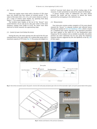
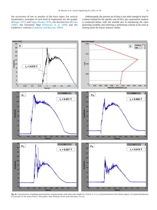
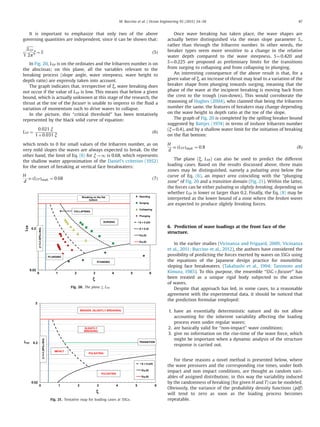
6. bottom (Fig. 9b) prior to splash up against the WEC (Fig. 9c) and
overtop the roof (Fig. 9d). Due to the intense dissipation of energy
and the large wave heights (Table 1), the reflection coefficient has
been found to be included between 0.10 and 0.56.
In the case of plunging breakers, the jet moves from the crest
(Fig. 10a); the wave profile behind the breaking area is then
horizontal or descending, whereas it was rising for surgings and
collapsings. In the present experiments the breaking initiated close
enough to the SSG, to allow the plunging jet slamming the
structure about its toe (Fig. 10b). After the “hammer shock”, an
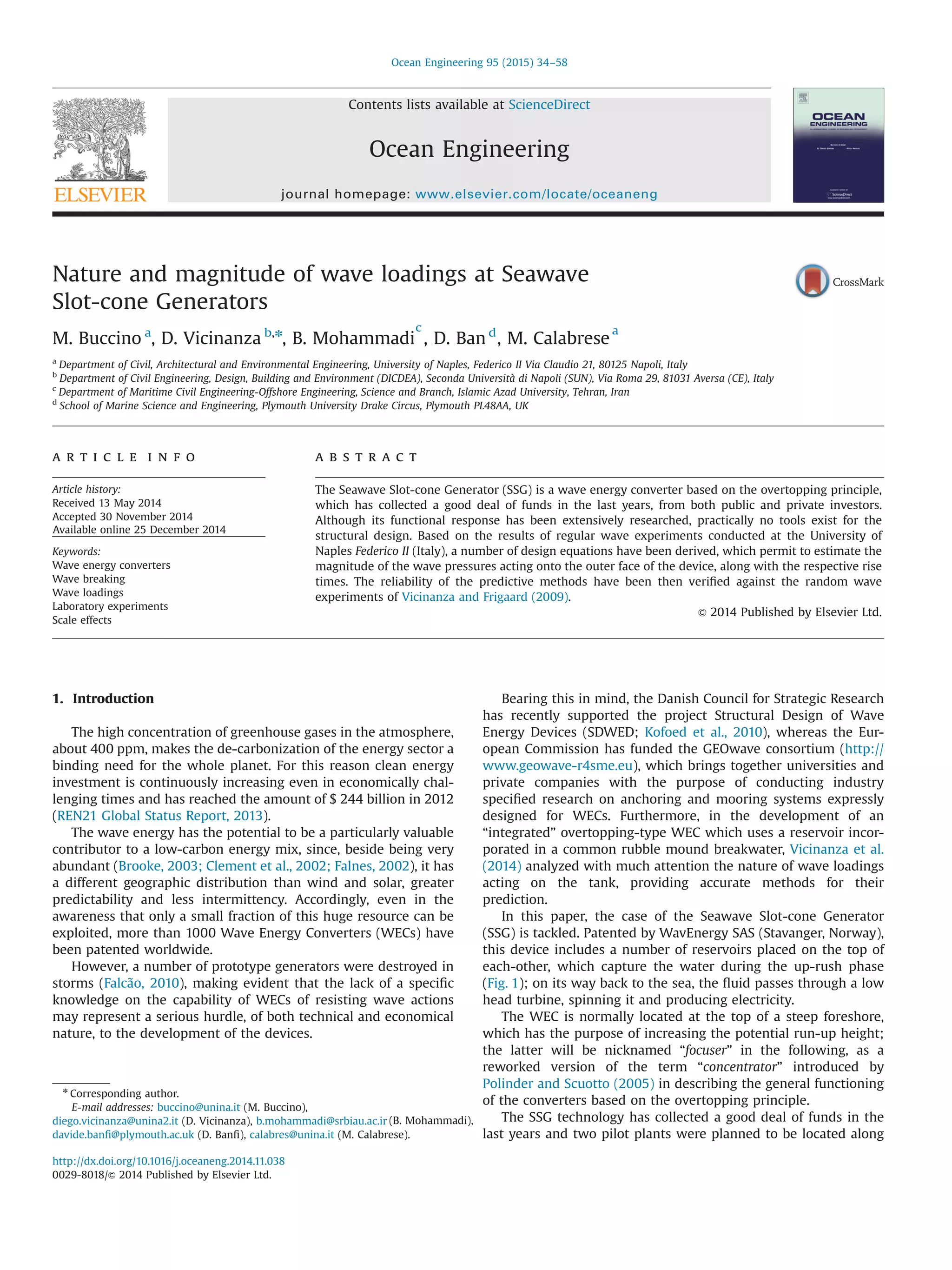
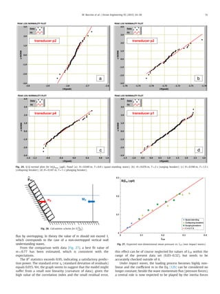
Fig. 8. Example of Surging breaker (H¼0.076 m, T¼2 s).
Fig. 9. Example of Collapsing breaker (H¼0.15 m, T¼1.5 s). The sketch reported in the upper left corner of panel “a” has been re-drawn from Galvin (1969).
Table 1
Summary of main hydraulic parameters. H refers to the measured values of the
incident wave heights.
#
tests
T[s] d
[m]
L
[m]
H [cm] kd H/L H/d Rc/H
8 0.80 0.50 0.99 4.92–12.25 3.17 0.050–0.124 0.10–0.24 0.82–2.03
8 1.00 0.50 1.51 3.59–15.42 2.08 0.024–0.102 0.07–0.31 0.65–2.78
8 1.50 0.50 2.78 3.56–21.92 1.13 0.013–0.079 0.07–0.44 0.46–2.80
7 2.00 0.50 4.02 2.58–16.21 0.78 0.006–0.040 0.05–0.32 0.61–3.87
M. Buccino et al. / Ocean Engineering 95 (2015) 34–58 39

7. intense splash-up is produced (Fig. 10c). The measured reflection
coefficients ranged from 0.15 to 0.58.
Both in case of plunging and collapsing breakers, an air pocket is
trapped beneath the plunging jet, which is then compressed and
destroyed by the incoming water mass.
4. Wave loadings macro-characteristics
4.1. General description
The actions produced by quasi-standing waves are of pulsating
(or quasi-static) type; this kind of loadings are dominated by the
effect of gravity and the rise times are of the same order as the
period of waves. Likely due to the low values of the wave
steepness tested (not larger than 0.04), the time-histories of the
wave force at the wall have been observed to possess the same
shape as the waves at the toe of the “focuser”. An example is given
in Fig. 11a, where the chronograms of the wave profile and Fint
have been standardized and limited to their positive part, to ease
the comparison. Together with forces also the pressures at the swl
have the same pulsating character (Fig. 11b).
The spatial distribution of pressures at the peak of force resulted
approximately bi-trapezoidal, with the maximum at the swl
(Fig. 11c); the vertical distance of the pressures barycentre from
the structure toe, ZG, has been found to not exceed 0.35 times the
wall height, hc (Fig. 11d).
However trivial it may seem, another remarkable feature of this
loading case is its repeatability under a regular wave attack; in the
example shown in Fig. 11e, more than 90% of the peaks of Fint are
included in the interval 3.9–4.1 kg/m, whereas the corresponding
rise-times lie in the range 0.2 T–0.23 T (Fig. 11f).
For surging and collapsing breakers with small wave heights, the
loading process remains quasi-static and repeatable, with a
pressure distribution at the peak of force still bi-trapezoidal
(Fig. 12 left panel). Yet, due to the wave overtopping, the centre
of mass of such distribution is located almost invariably at half the
structure height (Fig. 12 right panel). This is the same as supposing
the pressure to be constant along the SSG, in accordance to the
hypothesis formulated by Hiroi in the early '900 for vertical
breakwaters.
This analogy is most likely explained by the fact that in the
Japanese design practice, vertical breakwaters are allowed to be
significantly overtopped during the design storms (Goda, 1995).
With increasing the wave height, the big mass of water
involved in the process of up-rush attains such velocities and
accelerations to generate moderate impact events (^p still of the
order of H).
A deeper insight on the video camera recordings revealed that
as the steepness grows, the wave crest tends to reach quickly the
“breaking area” at the toe of the front, collapsing on it and then
hitting the wall (Fig. 13). The presence of foam and air bubbles
dampens the intensity of the impact.
This phenomenon, which is still relatively slow, causes the
appearance of a higher and sharper peak of force before the
pulsating smooth one (Fig. 14a). The ratio between the two
maxima may reach and overcome 2. At the same instant when
wave force reaches the peak, the maximum pressure is not
recorded at the swl, but above it (Fig. 14b). Depending on the
amount of water involved, the “impact” may be either localized
above the swl (with the lower pressures remaining pulsating) or
extend throughout the structure height, like in the case of the low
panels of Fig. 14.
Table 2
Details of pressure sensors positions.
Code Transducer centre to the SSG toe (cm) Description
p1 0.014 Toe of the SSG
p2 0.056 SWL
p3 0.094 Middle of 2nd plate
p4 0.132 Middle of 3rd plate
Fig. 10. Example of Plunging breaker (H¼0.11 m, T¼1.0 s).
M. Buccino et al. / Ocean Engineering 95 (2015) 34–5840

8. Under these conditions a real steady state seems to be not reached,
and accordingly repeatability is lost; under the same periodic attack,
small impacts may alternate to pulsating patterns.
It is noteworthy that the lack of repeatability applies also to the
spatial distribution of pressures, which may have the maximum either
at swl (pulsating events) or at different positions above it (Fig. 15a-c-e).
Yet, in spite of this variability, ZG seems to undergo, at the peak
of force, only slight fluctuations around the value 0.5 hc (Fig. 15b-
d-f). This result is rather interesting because, as partially men-
tioned before, would allow substituting the actual distribution of
loadings, highly variable, with its average value, that is expected to
be more stable and predictable. Nevertheless, given the low
number of pressure transducers here available, an accurate valida-
tion against new data sets is desirable. A first check is carried out
in the Section 7 of this article.
Under plunging breakers, the slamming of the plunging jet onto
the structure (hammer shock) generates a severe impulsive force
peak, as shown in Fig. 16a. When the maximum of Fint is reached,
the pressure magnitude at and above the swl is generally zero and
the spatial distribution of loadings might be assumed triangular,
with the maximum around the toe of the structure (Fig. 16b). The
impact event has a rise time extremely short (tr O(0.001 T)) and is
Fig. 11. Characteristics of loadings generated by quasi-standing waves (H¼0.036 m, T¼1.5 s). (a) time-histories of Fint and wave profile at the toe of the focuser; (b) time-
history of the wave pressure at the swl (in cm); (c) spatial distribution of loadings at the force peak (blue circles indicate extrapolated data); (d) time-history of the pressure
barycentre; (e) and (f) histograms of the peaks of force (in kg/m) and of the corresponding rise-time to wave period ratio.
M. Buccino et al. / Ocean Engineering 95 (2015) 34–58 41

9. followed by a number of oscillations due to the compression of the
air trapped during the crest overturning (see Fig. 10b).
Examining the pressure signals in the low panels of Fig. 16, it is
noted that the peaks of p2 and p3 are about one order of
magnitude lower than p1; this underlines the essentially local
nature of the loading case. Moreover, a sort of “secondary strike”,
much less intense than the main one, occurs at the transducer p4
because of the splash-up subsequent to the crest falling.
Since the impact mechanism is significantly affected by the amount
of air entertained in the water, and even by small disturbances of the
free surface (Peregrine, 2003), the resulting loadings exhibit a large
variance. A typical example is displayed in the histograms of Fig. 17,
which refer to the transducer p1 and the same experiment as in Fig. 16.
The pressure peaks (relative to H) and the corresponding rise time to
wave period ratios span over an entire order of magnitude; interest-
ingly, the modal value of the former is located between 1 and 2,
suggesting that violent impacts (peaks as large as 10 H) are in fact “tail
events” with low exceedance probability.
More generally, the impulsive pressure peaks measured in the
present experiments are significantly lower than those reported in
literature for vertical and sloping face breakwaters. For example, the
10% exceedance probability value of ^p=γHhas been found to not exceed
5, whereas Kirkgoz (1995) measured 14.5 on walls inclined by 451.
This big difference is mainly due to the macro-features of the
breaking process. While in the Kirkgoz experiments the waves arrived
almost flat at the structure, and the breaking initiated very close to the
wall with nearly no trapped air (the author referred to this situation as
perfect breaking), the impacts observed in the present tests occurred
well after the wave had begun to break, so that a significant amount of
air could be hold beneath the crest (Fig. 18).
This breaking morphology, which tends to reduce the risk of
violent impacts, is favored by two characteristics that are peculiar
of the SSG design, namely the shallow foreshore in front of the
structure and the relatively mild inclination of the outer plates;
the former causes the waves to attain the incipient breaking
condition prior reaching the wall, whereas the latter obliges the
breaker to perform a nearly 551 rotation to hit the structure.
4.2. Classification of wave forces
The patterns of wave force (Fint) previously described have been
grouped into three classes, based on the definitions introduced for
vertical breakwaters by the PROVERBS project (Oumeraci et al.,
1999; Allsop and Vicinanza, 1996; Allsop et al., 1996). Thus, a force
chronogram is termed pulsating if it exhibits a unique smooth peak
over a wave period. A double peak pattern is instead named either
slightly breaking or impact, depending on whether the first sharp
maximum is lower or larger than 2.5 times the second peak.
It is worth to point out that, owing to the inherent variability of
the force chronograms under breaking waves, the classification
above has been conventionally referred to the modal (most
frequent) features observed in each test.
5. Preliminary parametric analysis on breaker types and
loading cases occurrence
For maritime structures subjected to loadings of highly variable
nature, it is central to have a design tool which allows predicting
Fig. 12. Characteristics of loadings for a small collapsing breaker (H¼0.07 m, T¼1.5 s). Left panel: spatial distribution of pressures at the force peak (circles indicate
extrapolate values). Right panel: time-history of the pressures barycentre.
Fig. 13. Surging breaker with large wave height (H¼0.16 m, T¼2 s). Left panel: the crest of the wave reaches the dissipation area at the toe of the front. Right panel: the
water tongue hits the SSG and overtops the roof.
M. Buccino et al. / Ocean Engineering 95 (2015) 34–5842

10. the occurrence of one or another of the force types. For vertical
breakwaters, examples of such kind of implement are the graphs
of Nagai (1973) and Nagai-Otsubo (1974), the decision tree of Goda
(1986), the Parameter Map (Oumeraci et al., 1999) and the
Calabrese's criterion (Calabrese and Buccino, 2000).
Unfortunately, the present set of data is not wide enough to lead to
a robust method for the specific case of SSGs; yet, a parametric analysis
is conducted below, with the twofold aim of introducing the main
governing variables and achieving a preliminary scheme to be used as
starting point for future research works.
tr = 0.075 T
tr = 0.051 T tr = 0.060 T
tr = 0.027 T tr = 0.014 T
p1 p2
p3 p4
Fig. 14. Characteristics of loadings generated by a surging breaker with large wave height (H¼0.16 m, T¼2 s). (a) horizontal force time-history (kg/m); (b) spatial distribution
of pressures at the peak of force. Low panels: time-histories of the wave pressures (in cm).
M. Buccino et al. / Ocean Engineering 95 (2015) 34–58 43

11. The non-dimensional quantities employed are essentially three.
One is the well-known surf similarity parameter or inshore Iribarren
number (Battjes, 1974):
ξ ¼
tgαav:
ffiffiffiffiffiffiffiffiffiffiffiffiffiffiffiffiffiffiffiffi
2πH=gT2
q ð1Þ
in which H is the incident wave height at the toe of the focuser. As
for the slope at the numerator, the average value from the toe of
the bathymetry to the top of the SSG has been taken (tgαav.,
Fig. 19), to render the comparison with other data sets as simple
as possible. Compared to the average slope angle suggested by
Zanuttigh and Van der Meer (2008), who proposed to take the
mean between the points at71.5 H around the swl, tgαav also
accounts the inclination of the foreshore prior the breaking point,
which is important to distinguish among the various breaker
types. Furthermore, it allows maintaining bottom and wave
parameters separated in the Iribarren number of Eq. (1), thus
simplifying the interpretation of the results.
The second quantity is the (mean) “slope parameter” (Svendsen,
2006), which is widely used in literature for both wave propaga-
tion and wave reflection problems. It basically represents the ratio
Fig. 15. Force events for a surging breaker with large wave height (H¼0.16 m, T¼2 s).
M. Buccino et al. / Ocean Engineering 95 (2015) 34–5844

12. between the length of the waves and the mean horizontal distance
between the toe of the foreshore and the shoreline:
S ¼
tgαav:
kd
ð2Þ
In the Eq. (2), the wavenumber k has to be evaluated on the flat
bottom, where the still water depth equals d.
The third variable will be referred to as Linear Thrust Parameter
(LTP) hereafter and is a linearized- slightly-modified form of the
wave Momentum Flux Parameter (MFP) originally introduced by
Hughes (2004).
We consider the ratio between the maximum value (over a
wave period) of the cross-shore component of the wave momen-
tum flux through the base of the focuser (MF) and the correspond-
ing hydrostatic still water thrust (S0):
MF
S0
¼ ½maxŠt ϵ T
R η
À d pþρgzþρu2
À Á
dz
1
2ρgd
2
ð3Þ
where η is the free surface, z is the vertical coordinate (positive
upwards), u is the cross-shore wave velocity, ρ is the water density
and g is the gravity acceleration.
tr = 0.002 T
Impulsive peak
Quasi-static peak
Secondary impact
tr = 0.002 T
p1 p2
p3 p4
tr = 0.003 T
Fig. 16. Characteristics of loadings generated by a plunging breaker (H¼0.11 m, T¼1 s). (a) horizontal force time-history (kg/m); (b) spatial distribution of pressures at the
peak of force. Low panels: time-histories of the wave pressures (in cm).
M. Buccino et al. / Ocean Engineering 95 (2015) 34–58 45

13. Eq. (3) coincides with the definition of MFP, apart from the
introduction of the coefficient ½ at the denominator. By using the
linear wave theory and retaining only the first order terms, one gets:
LTP ¼
H
d
tanh kdð Þ
kd
ð4Þ
which in fact represents the excess of pressure thrust at the toe of the
slope due to the presence of waves. It is useful to remark that the
main difference between MFP and LTP is that the former is inherently
non-linear in H (Hughes 2004), whereas the latter is by definition. It
is finally noticed that in shallow waters LTP tends to the wave height
to depth ratio H/d.
Fig. 17. (a) Histogram of the peaks of pressure, relative to the incident wave height, for the transducer p1 (H¼0.11 m, T¼1 s). (b) histogram of the corresponding rise-time to
wave period ratio.
H 15cm T 1sH 14cm; T 1s
H 11cm T 0.8s H 12cm T 0.8s
Fig. 18. Examples of plunging breakers profiles at the structure.
S.W.L
αav
Fig. 19. Definition of the mean slope angle.
M. Buccino et al. / Ocean Engineering 95 (2015) 34–5846

14. It is important to emphasize that only two of the above
governing quantities are independent, since it can be shown that:
ffiffiffiffiffiffiffi
LTP
2π
r
ξ ¼ S ð5Þ
In Fig. 20, LTP is on the ordinates and the Iribarren number is on
the abscissas; on this plane, all the variables relevant to the
breaking process (slope angle, wave steepness, wave height to
depth ratio) are expressly taken into account.
The graph indicates that, irrespective of ξ, wave breaking does
not occur if the value of LTP is low. This means that below a given
bound, which is actually unknown at this stage of the research, the
thrust at the toe of the focuser is unable to impress to the fluid a
variation of momentum such to drive waves to collapse.
In the picture, this “critical threshold” has been tentatively
represented by the black solid curve of equation:
LTP ¼
0:021 ξ
1þ0:031 ξ
ð6Þ
which tends to 0 for small values of the Iribarren number, as on
very mild slopes the waves are always expected to break. On the
other hand, the limit of Eq. (6) for ξ-1 is 0.68, which represents
the shallow water approximation of the Daniel's criterion (1952)
for the onset of breaking at vertical face breakwaters:
H
d
LTPð Þshall: ¼ 0:68 ð7Þ
Once wave breaking has taken place, the wave shapes are
actually better distinguished via the mean slope parameter S.,
rather than through the Iribarren number. In other words, the
breaker types seem more sensitive to a change in the relative
water depth compared to the wave steepness. S¼0.420 and
S¼0.225 are proposed as preliminary limits for the transitions
from surging to collapsing and from collapsing to plunging.
An interesting consequence of the above result is that, for a
given value of ξ, an increase of thrust may lead to a variation of the
breaker shape from plunging towards surging, meaning that the
phase of the wave at the incipient breaking is moving back from
the crest to the trough (run-down). This would corroborate the
reasoning of Hughes (2004), who claimed that being the Iribarren
number the same, the features of breakers may change depending
on the wave height to depth ratio at the toe of the slope.
The graph of Fig. 20 is completed by the spilling breaker bound
suggested by Battjes (1974) in terms of inshore Iribarren number
(ξ¼0.4), and by a shallow water limit for the initiation of breaking
on the flat bottom:
H
d
LTPð Þshall: ¼ 0:8 ð8Þ
The plane (ξ, LTP) can also be used to predict the different
loading cases. Based on the results discussed above, three main
zones may be distinguished, namely a pulsating area below the
curve of Eq. (6), an impact area coinciding with the “plunging
zone” of Fig. 20 and a transition domain (Fig. 21). Within the latter,
the forces can be either pulsating or slightly breaking, depending on
whether LTP is lower or larger than 0.2. Finally, the Eq. (8) may be
interpreted as the lower bound of a zone where the broken waves
are expected to produce slightly breaking forces.
6. Prediction of wave loadings at the front face of the
structure.
In the earlier studies (Vicinanza and Frigaard, 2009; Vicinanza
et al., 2011; Buccino et al., 2012), the authors have considered the
possibility of predicting the forces exerted by waves on SSGs using
the equations of the Japanese design practice for monolithic
sloping face breakwaters. (Takahashi et al., 1994; Tanimoto and
Kimura, 1985). To this purpose, the ensemble “SSGþfocuser” has
been treated as a unique rigid body subjected to the action
of waves.
Despite that approach has led, in some cases, to a reasonable
agreement with the experimental data, it should be noticed that
the prediction formulae employed:
1. have an essentially deterministic nature and do not allow
accounting for the inherent variability affecting the loading
process even under regular waves;
2. are basically valid for “non-impact” wave conditions;
3. give no information on the rise-time of the wave force, which
might be important when a dynamic analysis of the structure
response is carried out.
For these reasons a novel method is presented below, where
the wave pressures and the corresponding rise times, under both
impact and non impact conditions, are thought as random vari-
ables of assigned distribution; in this way the variability induced
by the randomness of breaking (for given H and T) can be modeled.
Obviously, the variance of the probability density functions (pdf)
will tend to zero as soon as the loading process becomes
repeatable.
0.02
0.2
0 1 2 3 4 5 6
LTP
Standing
Surging
Collapsing
Plunging
S = 0.225
S = 0.42
Eq.(6)
Eq.(8)
STANDING
COLLAPSING.
ξ=0.4(SPILLING)
Breaking on the flat
bottom
SURGING
PLUNGING
ξ
Fig. 20. The plane ξ, LTP.
0.02
0.2
2
0 1 2 3 4 5 6
LTP
S = 0.225
Eq.(6)
Eq.(8)
PULSATING
BROKEN (SLIGHTLY BREAKING)
IMPACT
PULSATING
SLIGHTLY
BREAKING
TRANSITION
ξ=0.4(SPILLING)
ξ
Fig. 21. Tentative map for loading cases at SSGs.
M. Buccino et al. / Ocean Engineering 95 (2015) 34–58 47

15. 6.1. General assumptions and simplifications
At the instant of force peak, the pressures distribution onto the
front face of the device is assumed uniform, with a magnitude, ^pav.,
equal to the average pressure along the wall (Fig. 22, left part). The
latter has been calculated dividing the peak of the horizontal
component of Fint (e.g. Figs. 14 and 16) by the height of the WEC,
hc. The single force events are approximated to triangular pulses of
duration equal to twice the measured rise time tr (Fig. 22, right part).
The results of previous sections indicate that a rectangular
distribution of pressures leads to a realistic estimate of the force
application point for non-impacting waves with significant over-
topping, which is the most frequent design situation; in the other
cases this assumption is cautious, as it wreaks an over-prediction
of the overturning moment about the structure heel.
Along with the mean value, in the following also the maximum
of the pressure distribution, ^pmax, is considered; this quantity, not
dealt with in the previous research, is central to assess the
thickness of the outer plates of SSG.
The location of ^pmax has to be individuated necessarily on
statistical basis, since it has been seen that under the same regular
wave train the distribution of loadings may change from event to
event (Fig. 15).
Here we assume this position coincides with that of the transdu-
cer where the maximum modal value of the peak pressure (^pÞ has been
recorded. The mode has been estimated from the histogram of ^p (e.g.
Fig. 17), using a number of bins in accordance with the Stegun's rule.
Obviously, the extrapolated values at the ends of the wall (top and
toe) have been not considered in this phase.
6.2. The joint probability distribution of ^pav. and tr
It has been observed that for a given wave height and period,
the joint probability density function (j-pdf ) of ^pav. and tr can be
reasonably assumed to be a bivariate log-normal. The distribution
can be written as:
f Xð Þ ¼ 2πΣ
À 0:5
exp À1
2 X Àμ
À Át
ΣÀ1
X Àμ
À Án o
ð9Þ
in which X is the vector of the “log-variables”, μ is the vector of
averages and Σ is the matrix of covariance. Here we set:
X ¼ X1; X2ð Þ ¼ ln
^pav:
ρgd
; ln
tr
T
!
ð9aÞ
μ ¼ μX1
; μX2
ð9bÞ
Σ ¼
σ2
X1
rσX1
σX2
rσX2
σX1
σ2
X2
0
@
1
A ð9cÞ
where mXi and σXi represent the mean and standard deviation of
the marginals and r is the correlation coefficient.
In the examples displayed in Figs. 23 and 24, the top panels
(a and b) report the Q-Q plots of the variables X1 and X2; this to
show the marginals are individually Gaussian (necessary but not
sufficient condition to the bivariate normality).
Then, the Chi-square probability plot of the sample values of the
quantity X Àμ
À Át
ΣÀ1
X Àμ
À Á
is given in the panel c, to demonstrate
that X1 and X2 are also jointly normal; it has been argued by
Johnson and Wichern (1998) that in a bivariate normal random
vector, the quantity above has a chi-square probability distribution
with 2 degrees of freedom. Thus, if the points in panel c tend to fall
along a straight line, our hypothesis cannot be rejected.
The figures are completed with the confidence ellipse of
equation:
X Àμ
À Át
ΣÀ1
X Àμ
À Á
¼ χ2
2 0:05ð Þ ð10Þ
which should contain approximately the 95% of data (panel d), and
with a 3D view of the fitted bivariate surface (panel e), along with
its contour-lines (panel f).
6.3. The probability density function of ^pmax.
Analogously to ^pav., also the maximum peak pressure can be
reasonably described through a log-normal distribution. Fig. 25
shows four examples of Q–Q plot of the variable ln ^pmax:=ρgd
À Á
;
each panel corresponds to a different wave shape, i.e. quasi-
standing, surging, collapsing and plunging. From the graph one
can easily realize how the variance of the loading process
increases passing from quasi-standing waves to plunging breakers.
It is worth noticing that in both the present and the previous
paragraph, the log-normal distribution is used for all the variables
under both impact and non impact conditions; this represents in
fact a generalization of the approach employed by Fuhrboter
(1985), Kirkgoz (1995), Vicinanza (1997), Calabrese et al. (2000)
and many others, where such a pdf was fitted only to the impulsive
peak pressures.
After establishing the probabilistic models, the problem boils
down to the estimation of parameters. Overall they are seven,
namely the mean and standard deviation of ^pav and tr (4 para-
meters), their correlation coefficient (r) and the mean and stan-
dard deviation of ^pmax.
pmax
pav
Fh
t
2tr
pav hc
hc
Fig. 22. Simplified loading scheme.
M. Buccino et al. / Ocean Engineering 95 (2015) 34–5848

16. In the next paragraphs, a set of equations are proposed, where
those quantities are predicted in function of the governing vari-
ables introduced in Section 5.
6.4. The mean of ^pav
Under non-impact conditions a crude predictive model has been
developed, which employs an approach conceptually similar to
that used by Tanimoto and Kimura (1985) for trapezoidal walls.
Assuming that the device and the steep foreshore behave like a
unique structure (Fig. 26), from the conservation of the horizontal
momentum follows that the maximum horizontal momentum flux
of the incoming waves at the toe of the focuser (MF) should equal
the horizontal component of the peak force exerted onto the
structure (Πx). Under the hypothesis of uniform distribution of
pressures we have:
Πx ¼ ^pav: dþRcð Þ ¼ MF ð11Þ
Now we linearize the previous equation retaining only the
pressure term in MF (see Eq. (3)) and noting that in the case of
SSGs it can be assumed that Rc is of the order O(H); accordingly,
the product ^pav: Rc
À Á
is of order O H2
and can be neglected.
Fig. 23. Bivariate log-normal plots for H¼0.113 m, T¼0.8 s (plunging breaker). (a) the log-normal plot for lnð^pav:=ρgdÞ; (b) the log-normal plot for lnðtr:=TÞ; (c) the Chi-square
probability plot of the sample values of the quantity X Àμð Þt
Σ À 1
X Àμð Þ;(d) the confidence ellipse; (e) 3D view of the fitted bivariate surface; (f) contour-lines of the curve.
M. Buccino et al. / Ocean Engineering 95 (2015) 34–58 49

17. Thus, after taking the average over a given experiment we
obtain:
E ^pav:
À Á
¼
MF
d
¼ ρg
H
2
tanh kdð Þ
kd
ð11bÞ
In which E(1) represents the expectation operator. The latter
does not appear at the right hand side of Eq. (11b), since,
oppositely to the wave pressure, the variance of H and T within
the same regular wave train can be neglected. After dividing both
sides by ρgd one finally gets:
E
^pav:
ρgd
¼
1
2
LTP ð12Þ
or more generally:
E
^pav:
ρgd
¼ m LTP ð12bÞ
where the coefficient m accounts for the main terms neglected in the
balance, namely wave reflection, inertia forces and loss of momentum
Fig. 24. Bivariate log-normal plots for H¼0.128 m, T¼1.5 s (collapsing-breaker). (a) the log-normal plot for lnð^pav:=ρgdÞ; (b) the log-normal plot forlnðtr:=TÞ; (c) the Chi-
square probability plot of the sample values of the quantity X Àμð Þt
Σ À 1
X Àμð Þ ;(d) the confidence ellipse; (e) 3D view of the fitted bivariate surface; (f) contour-lines of
the curve.
M. Buccino et al. / Ocean Engineering 95 (2015) 34–5850

18. flux by overtopping. In theory the value of m should not exceed 1,
which corresponds to the case of a non-overtopped vertical wall
understanding waves.
From the comparison with data (Fig. 27), a best fit value of
m¼0.77 has been estimated, which is consistent with the
expectations.
The R2
statistics exceeds 0.95, indicating a satisfactory predic-
tion power. The standard error se (standard deviation of residuals)
equals 0.015. Yet, the graph seems to suggest that the model might
suffer from a small non linearity (curvature of data); given the
high value of the correlation index and the small residual error,
this effect can be of course neglected for values of LTP within the
range of the present data set (0.03–0.32), but needs to be
accurately checked outside of it.
Under impact waves, the loading process becomes highly non-
linear and the coefficient m in the Eq. (12b) can be considered no
longer constant; beside the wave momentum flux (pressure forces),
a central role is now expected to be played by the inertia forces
transducer p2 transducer p2
transducer p4 transducer p1
Fig. 25. Q-Q normal plots for ln(^pmax :/ρgd). Panel (a): H¼0.049 m, T¼0.8 s (quasi-standing wave); (b): H¼0.076 m, T¼2 s (surging breaker); (c) H¼0.198 m, T¼1.5 s
(collapsing breaker); (d) H¼0.147 m, T¼1 s (plunging breaker).
pav
MFπX
Fig. 26. Calculation scheme for E
^pav:
ρgd
.
Fig. 27. Expected non-dimensional mean pressure vs. LTP (non impact waves).
M. Buccino et al. / Ocean Engineering 95 (2015) 34–58 51

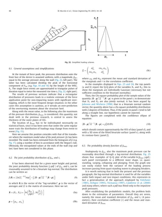
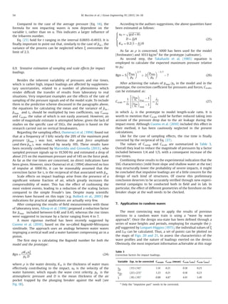
19. which, according to the linear wave theory, are proportional to the
wave steepness. For this reason m is supposed to be a decreasing
function of the Iribarren number, which can be roughly viewed as
the ratio between the along-slope components of the gravity forces
(representing a resistance to the wave motion) and the inertia
forces. The following expression is proposed:
E
^pav:
ρgd
¼ 2:68 ξÀ 2:42
h i
LTP ð13Þ
with R2
¼0.90 and se¼0.025. Caution is recommended in using the
above formula outside the range:
0:015r ξÀ2:42
LTP r0:108 ð13bÞ
Fig. 28 shows the comparison between calculated and mea-
sured value of E ^pav:=ρgd
À Á
6.5. The standard deviation of ^pav
The standard deviation of the non-dimensional mean pressure
is significantly influenced by the Iribarren number. Fig. 29 clearly
shows a decrease of variability with increasing ξ, so that the
loading process can be considered practically repeatable beyond
the Iribarren and Nogales (1949) breaking limit ξ¼2.3. According
to Battjes (1974), the latter tends in fact to separate a zone of
complete breaking (high variability) from a zone about halfway
between breaking and reflection (quasi-standing waves and sur-
ging breakers with low variability of ^pav).
However, for a given ξ the occurrence and intensity of wave
breaking have been seen to be also affected by the linear thrust
parameter LTP; as the latter increases, the waves pass first from
non-breaking to breaking and once the rupture has taken place,
the scales of dissipation tend to progressively increase. This
definitely leads the variance of the process to raise.
Then, for a more effective prediction, the following equations
are suggested:
ffiffiffiffiffiffiffiffiffiffiffiffiffiffiffiffiffiffiffiffiffiffiffiffiffi
VAR
^pav
ρgd
s
¼
0:0012þ0:0474 uþ0:8017 u2
ðnon impact waves R2
¼ 0:93 Þ
0:0009exp 10:39 tð Þ ðimpact waves R2
¼ 0:89Þ
(
ð14Þ
where:
u ¼ LTP
ξ0:6
t ¼
L0:3
TP
ξ
8
:
ð15Þ The standard error is respectively 0.013 and 0.026.
Eq. (14) indicates that the Iribarren number is the most
important parameter under impact conditions, whereas LTP dom-
inates under non impacting waves. The application ranges of the
formulae are:
0:0157rur0:2600
0:2407 rtr0:4933
(
ð16Þ
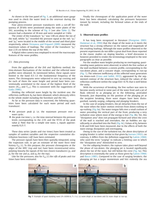
6.6. The non dimensional rise time tr/T
Under non impact conditions, the average of the marginal pdf of
the force rise time to wave period ratio can be estimated as
(Fig. 30):
E
tr
T
!
¼ 0:21 tanh
π
22 u
R2
¼ 0:80se ¼ 0:019
ð17Þ
As expected, Eq. (17) tends to 0.21 (theoretical value for sine
waves) as the Iribarren number grows and/or the momentum flux
decreases.
0
0.05
0.1
0.15
0.2
0.25
0.3
0 0.1 0.2 0.3
measured
predicted
Fig. 28. Measured vs. predicted E
^pav:
ρgd
for impact waves.
0
0.03
0.06
0.09
0.12
0.15
0.18
0 1 2 3 4 5 6
st.deviation
Quasi-Standing
Surging breakers
Collapsing breakers
Plunging breakers
Iribarren and Nogales
ξ
Fig. 29. Standard deviation of
^pav:
ρgd
vs. the Iribarren number.
0
0.05
0.1
0.15
0.2
0.25
0 10 20 30 40 50 60 70 80
E[tr/T]
1/u
Fig. 30. Mean of the non-dimensional force rise-time vs. Eq. (17). Non
impact waves.
M. Buccino et al. / Ocean Engineering 95 (2015) 34–5852

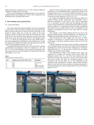
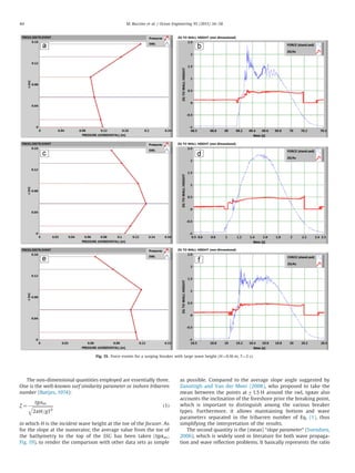
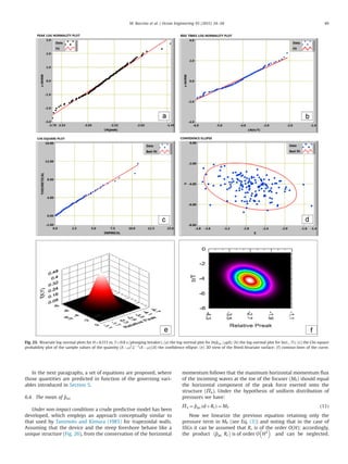
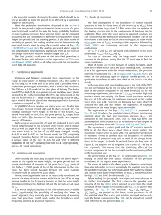
20. On the other hand, for impact conditions the following rela-
tionship has been found (Fig. 31):
E
tr
T
!
¼ 0:023ξ2:94
R2
¼ 0:86 se ¼ 0:009; 1rξr1:85
ð18Þ
As far as the standard deviations are concerned, the following
approximate equations may be used:
ffiffiffiffiffiffiffiffiffiffiffiffiffiffiffiffiffiffiffiffi
VAR
tr
T
s
¼
0:011 exp 6:09 u½ Š non impact waves; R2
¼ 0:53 se ¼ 0:0124
1:14 E tr
T
À Á
ðimpact wavesÞ
8
:
ð19Þ
The second of the above formulae simply states that the
marginal pdf of the non dimensional rise-time of the wave force
has a 114% variation coefficient under impact events. This does
underline the extreme instability of this kind of phenomenon.
It could be finally useful to remark that the Eq. (17) and the first
of the Eq. (19) are valid in the range defined by the first of the
Eq. (16).
6.7. The linear correlation coefficient, r
The linear correlation coefficient, which links X1 and X2 in
Eq. (9a), can be crudely estimated as follows:
r ¼
0:025 quasiÀstanding waves; se ¼ 0:12ð Þ
0:662 lnξÀ0:505 ðbreaking waves; R2
¼ 0:73 se ¼ 0:15Þ
(
ð20Þ
The second of the previous formulae holds for values of the
Iribarren number included between 1 and 4.
It should be noticed that for plunging breakers, corresponding
to low values of ξ, the correlation coefficient becomes rather
negative (around À0.45). This because, as argued by a number of
authors (e.g. Bagnold, 1939; Hattori and Arami, 1992), the impulse
of wave loadings tends to conserve oneself under impact condi-
tions. On the other hand, force and rise-time seem nearly un-
correlated under non-breaking waves, such that their joint pdf
tends to the simple product of the marginals.
6.8. Mean and variance of the maximum pressure ^pmax
Under non impact conditions, the use of the simple linear
relationship of Eq. (12b) revealed itself effective only for large
LTPs, say beyond 0.15. For smaller values, a non-linear term has to
be introduced. Thus, the following predictive model is proposed:
E
^pmax
ρgd
¼
m LTP
m ¼ max 2:275 exp À4:68 LTPð Þ; 1:03½ Š
(
ð21Þ
which, as shown in Fig. 32, leads to an excellent agreement with
data (R2
¼0.98, se¼0.011).
Under plunging breakers, the factor m is again assumed to be a
decreasing function of the Iribarren number. This led to (Fig. 33):
E
^pmax :
ρgd
¼ 10:19ξÀ 2:77
h i
LTP R2
¼ 0:92; se ¼ 0:082
ð22Þ
which should be cautiously used within the range:
0:012rξÀ 2:77
LTP r0:103 ð22bÞ
As far as the standard deviations are concerned, the following
expressions are suggested:
ffiffiffiffiffiffiffiffiffiffiffiffiffiffiffiffiffiffiffiffiffiffiffiffiffiffiffiffi
VAR
^pmax :
ρgd
s
¼
max 0:095 t; 0:352t À0:084½ Š non impact waves R2
¼ 0:95
0:0046exp 9:98 tð Þ impact waves R2
¼ 0:88
8
:
ð23Þ
with a standard error of respectively 0.007 (non impact) and 0.093
(impact).
0
0.03
0.06
0.09
0.12
0.15
0.9 1.1 1.3 1.5 1.7 1.9
E[tr/T]
ξ
Fig. 31. Mean of the non-dimensional force rise-time vs. Eq. (18). Impact waves.
0
0.1
0.2
0.3
0.4
0 0.1 0.2 0.3 0.4
Measured mean
Predicted mean
Data
Perfect agreement
Fig. 32. Measured vs. predicted E
^pmax :
ρgd
for non impact waves.
0
0.2
0.4
0.6
0.8
1
1.2
0 0.2 0.4 0.6 0.8 1 1.2
Measured mean
Predicted mean
Data
Perfect agreement
Fig. 33. Measured vs. predicted E
^pmax :
ρgd
for impact waves.
M. Buccino et al. / Ocean Engineering 95 (2015) 34–58 53

21. Compared to the case of the average pressure (Eq. 14), the
formula for non impacting waves is now dependent on the
variable t, rather than on u. This indicates a larger influence of
the Iribarren number.
Eq. (23) hold for t ranging in the interval 0.0693–0.4933. It is
finally important to point out that, similarly to the case of ^pav:, the
variance of the process can be neglected when ξ overcomes the
limit of 2.3.
6.9. Tentative estimation of sampling and scale effects for impact
loadings.
Besides the inherent variability of pressures and rise times,
which is rather high, impact loadings are affected by supplemen-
tary uncertainties, related to a number of phenomena which
render difficult the transfer of results from laboratory to real
situations. Very important examples are the effects of the rate of
sampling of the pressure signals and of the model scale. To include
them in the predictive scheme discussed in the paragraphs above,
the equations for calculating the mean and the variance of ^pav:,
^pmax : and tr, should be multiplied by two coefficients, say Csamp.
and Cscale, the value of which is not easily assessed. However, an
order of magnitude estimate is attempted below; given the lack of
studies on the specific case of SSGs, the analysis is based on the
research carried out on vertical breakwaters.
Regarding the sampling effect, Oumeraci et al. (1994) found out
that at a frequency of 1 kHz nearly the 20% of the maximum peak
pressure (^pmax :Þ was lost, whereas the peak force amplitude
ðand then ^pav:Þ, was reduced by nearly 10%. These results have
been recently confirmed by Marzeddu and Gironella (2013), who
sampled pressure signals up to 19,500 Hz and estimated a drop of
about 21% on the maximum pressure and of 14% on the force peak.
As far as the rise times are concerned, no direct indications have
been given. However, since Oumeraci et al. (1994) observed no loss
of impulse at 1000 Hz, it can be reasonably assumed that the
correction factor for tr is the reciprocal of that associated with ^pav:
Scale effects on impact loadings arise from the presence of a
significant volume fraction of air, which greatly increases the
compressibility of water. This has the effect of cushioning the
most violent events, leading to a reduction of the scaling factors
compared to the simple Froude's law. Despite many scientific
reviews have focused on this topic (e.g. Bullock et al., 2001) the
indications for practical applications are actually very few.
After comparing the results of field measurements with those
of laboratory tests, Allsop et al. (1996) proposed a reduction factor
for ^pmax : included between 0.40 and 0.45, whereas the rise times
were suggested to increase by a factor ranging from 4 to 7.
A more rigorous method has been recently suggested by
Cuomo et al. (2010), based on the so-called Bagnold-Mitsuyasu
similitude. The approach uses an analogy between water waves
impinging a vertical wall and a water hammer compressing air in a
piston.
The first step is calculating the Bagnold number for both the
model and the prototype:
Bgn ¼
ρKwu2
0
p0 D
ð24Þ
where ρ is the water density, Kw is the thickness of water mass
effectively contributing to the impact, u0 is the velocity of the
water hammer, which equals the wave crest celerity, p0 is the
atmospheric pressure and D is the mean thickness of the air
pocket trapped by the plunging breaker against the wall (see
Fig. 18).
According to the authors suggestions, the above quantities have
been estimated as follows:
u0 ¼
ffiffiffiffiffiffiffiffiffiffiffiffiffiffiffiffiffi
g dþHð Þ
p
D ¼ π
12H
Kw ¼ 0:2 1À π
12
À Á
H
8
:
ð25Þ
As far as ρ is concerned, 1000 has been used for the model
(freshwater) and 1033 kg/m3
for the prototype (saltwater).
As second step, the Takahashi et al. (1985) equation is
employed to calculate the expected maximum pressure relative
to p0:
Bgn ¼ 5
pmax
p0
2=7
þ 2
pmax
p0
À5=7
À7 ð26Þ
After achieving the values of pmax=p0 in the model and in the
prototype, the correction coefficient for pressures and forces, Cscale,
can be estimated as:
Cscale ¼
1
λF
pmax
p0
Prot:
À1
pmax
p0
mod:
À1
2
6
4
3
7
5 ¼
λS
λF
ð27Þ
in which λF is the prototype to model length-scale ratio. It is
worth to mention that Cscale could be further reduced taking into
account of the pressure drop due to the air leakage during the
impact event. Although Cuomo et al. (2010) included this effect in
their method, it has been cautiously neglected in the present
calculations.
Like for the case of sampling effects, the rise time is finally
corrected by the reciprocal of Eq. (27).
The values of Csamp. and Cscale are summarized in Table 3.
Overall they lead to reduce the magnitude of pressures by a factor
included between 1/4 and 1/5, with a consequent increase of the
rise-times.
Combining these results to the experimental indication that the
SSG characteristics (mild front slope and shallow water at the toe)
may structurally lower the probability of severe impacts, it might
be concluded that impulsive loadings are of a little concern for the
design of such kind of structures. Of course this preliminary
conclusion deserves to be accurately verified through new experi-
mental campaigns to be conducted both in field and in lab. In
particular, the effect of different geometries of the foreshore on the
breaker shape at the wall needs to be checked.
7. Application to random waves
The most convincing way to apply the results of previous
sections to a random wave train is using a “wave by wave
approach”. Once the design sea-state has been defined through a
series of wave heights and periods, employing for example the j-
pdf suggested by Longuet-Higgins (1975), the individual values of ξ
and LTP can be calculated. Thus, a set of points can be plotted on
the maps of Figs. 20 and 21, to assess the characteristics of the
wave profiles and the nature of loadings exerted on the device.
Obviously, the most important information achievable at this stage
Table 3
Correction factors for impact loadings.
Variable Eqs. to be corrected Csample Cscale (mean) Cscale (min) Cscale (max)
^pav:
ρgd
(13)–(14)a
1.14 0.21 0.18 0.23
^pmax :
ρgd
(22)–(23)a
1.23 0.21 0.18 0.23
tr
T
(18)–(19)a
0.88 4.87 4.41 5.49
a
Only the “impulsive part” needs to be corrected.
M. Buccino et al. / Ocean Engineering 95 (2015) 34–5854

22. is the expected number of plunging breakers, which should be as
low as possible to avoid the project to be affected by a significant
degree of uncertainty.
Then, the probability distributions discussed in the Section 6
should be interpreted as pdfs conditional to the occurrence of a given
wave height and period; in this way, the design probability functions
of wave loadings (pressure, force and rise times) can be estimated
accounting for the randomness of both the wave parameters (wave
height and period) and the breaking process. If the latter source of
variability is ignored, the loading variables can be deterministically
associated to each wave by using the expected values of Eqs. (12),
(13),(17),(18),(21) and (22). The analysis presented above suggests
this simplification to be rigorously appropriate when all the waves of
the design storm have Iribarren numbers larger than 2.3.
The first (partial) verification of the described procedure is
discussed below with reference to the experiments of Vicinanza
and Frigaard (2009), which, as of today, represent the sole random
wave data-set available.
7.1. Description of experiments
Vicinanza and Frigaard conducted their experiments at the
“Deep 3D wave basin” of Aalborg University (DK). The facility is
15.7 m long, 8.5 m wide and 1.5 m deep and is provided with a
snake-front piston type wavemaker, with a total of ten actuators.
The SSG was a 1:60 model of the pilot plant of Kvitsøy. The device
was 0.097 m high (5.82 m in prototype) and had three outer plates
inclined by 351 to the horizontal. The WEC has been seated on the
top of a focuser with a 1:1 slope (rocky cliff), giving a value of tgαav.
equal to 0.84. The front plates have been equipped with 9 pressure
transducers sampled at 200 Hz.
32 JONSWAP driven random sea states were run, divided into
two groups: 16 long crested (2D) and 16 short crested (3D). The
spectral significant wave height at the toe of the focuser, Hm0,
varied from 0.042 m to 0.25 m; the peak period, Tp, ranged from
1.03 s to 2.07 s. The duration of the wave attacks was approxi-
mately 1000 waves.
Each group of experiments (2D and 3D) included 8 tests with
waves perpendicular to the structure (front waves) and 8 oblique
attacks with an angle of 451 (side waves). In the 2D experiments,
two water levels at the toe of the cliff were changed, namely
d¼0.50 m and d¼0.53 m; the former made the SSG completely
exposed (shoreline device). 3D tests were instead performed with
a unique value of the swl (d¼0.53 m) and with 2 different
exponents of the cos2n
spreading function: n¼4 (large spreading)
and n¼10 (small spreading).
7.2. Limitations and assumptions
Unfortunately the only data available from the above experi-
ments is the significant wave height, the peak period and the
spatial distribution of pressures at the peak force ^F1/250 (mean of
the highest 1/250th peaks of force). No information on the rise-
times has been stored, basically because the wave loadings
recorded could be considered quasi-static.
Hence, some hypotheses have to be necessarily introduced; we
assume the wave elevation process at the toe of the cliff to be very
narrow banded in the frequency domain, so that the wave height
distribution follows the Rayleigh pdf and the periods are all equal
to Tp.
It is worth emphasizing that if the little information available
limits (significantly) the possibility of verifying the “wave by
wave” approach, they ironically give the opportunity of assessing
how that procedure might work under the hypotheses most
frequently adopted by practical engineers.
7.3. Results of comparison
The first consequence of the hypothesis of narrow banded
spectrum is that for these tests all the waves up to H1/250 have
Iribarren numbers larger than 2.3. This means that the variance of
the loading process due to the randomness of breaking can be
neglected. Then, since the wave period is assumed constant, we
can conclude that the cumulative distribution function (cdf) of the
wave forces is the same as that of the wave heights; in other words
H1/250 gives rise to ^F1/250, according to the approach followed by
Goda (1986) and commonly accepted in the engineering
applications.
In Fig. 34 ξ and LTP are calculated with reference to the wave
parameters H1/250 ¼1.8 Hm0 and Tp.
For sake of clearness only the long-crested wave data is
reported in the picture, seeing that the 3D tests have in fact the
same coordinates.
Most of points are in the domain of surging breakers, apart
from two of them which fall in the quasi-standing zone. This result
is in a fair agreement with the visual observations; the pressure
patterns recorded (see Fig. 7 of Vicinanza and Frigaard (2009)) are
either of the pulsating type or slightly double-peaked, in a
qualitative accordance to what described in the Section 4 of this
article.
In the two tests with non-breaking waves, the roof of the WEC
was not overtopped, due to the low value of the wave thrust at the
base of the focuser compared to the crest freeboard. As for the
remaining experiments, the values of (LTP)1/250 are rather high and
produce severe overtopping; the linear thrust parameter reaches
the level of 0.76, whereas the maximum measured in the regular
wave tests was 0.32. However, no breaking has been observed
seaward the cliff and this makes the hypothesis of Rayleigh
distribution of the wave heights quite reasonable.
The application of the Eqs. (12b) and (21) is presented in
Figs. 35 and 36 where the predicted values of force, overturning
moment about the heel and maximum pressure (^pmax :) are
compared to the measured ones. The 3D data has been not
parameterized with respect to n, as no influence of the degree of
spreading has been detected (Vicinanza and Frigaard, 2009).
The agreement is rather good and the R2
statistics exceeds
0.95 in all the three cases. Apart from a single outlier, the
maximum relative error is about 20%. The satisfactory prediction
of moments seems to confirm that the hypothesis of uniform
distribution of pressures may suit to most of the design situa-
tions. In this respect it should be noticed that in the low panel of
Figure B, the torques are all negative (the values of “–M”are in
fact reported). This means that the stabilizing effect of the
vertical component of the force prevails on the overturning effect
of the horizontal one.
The performance of the Eq. (21) is surprisingly good (Fig. 36)
bearing in mind the low spatial resolution of the pressure
transducers in the regular wave experiments.
The scatter of points in the above graphs is however some larger
than what inferred in Section 6; accordingly, the standard error (se) of
the predictive formulae has to be recalculated. After gathering regular
and random wave data (49 experiments on total) se resulted 0.026 for
the Eqs. (12b) and 0.043 for the formula (21).
Before ending this paragraph, two important issues deserve to
be further investigated. The first concerns the possible non
linearity of the Eq. (12b), which seemed to arise from the small
curvature of the regular wave points in the Fig. 27. To answer this
question, in Fig. 37 the residuals eipav ¼ ^pav:=ρgd
À Á
meas:
À
^pav:=ρgd
À Á
calc:
are plotted vs. the linear thrust parameter for all
the available data. The scatter plot exhibits no trend and accord-
ingly the linear relationship of Eq. (12b) can be considered correct
with reference to the present data set.
M. Buccino et al. / Ocean Engineering 95 (2015) 34–58 55

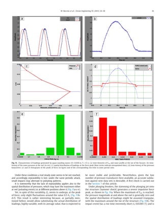
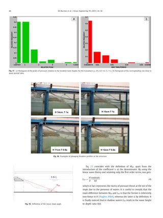
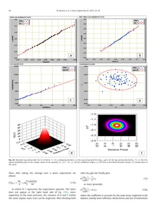
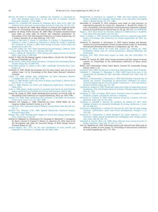
23. Yet, it can be observed a certain tendency at underpredicting
the 2D tests and overpredicting the 3D ones. This is the conse-
quence of the fact that short-crested waves induce loadings
slightly smaller, being the wave parameters the same. However,
the issue has been considered of little relevance given the very
good quality of the estimates.
The second point of interest is that the Eqs. (12b) and (21) have
been applied to both front and side waves, introducing no
obliquity correction. From a physical point of view this is consis-
tent, because the wave momentum flux (LTP), which is supposed to
generate these non impact loadings, includes only the pressure
term and is then independent of the wave direction. To verify the
correctness of this assumption, in Fig. 38 the residuals of the non
dimensional mean and maximum pressures are plotted against the
angle of propagation of waves (random wave tests only). Since
again no trend is observed, it can be concluded that the present
data set does not contradict the hypothesis formulated.
8. Conclusions
The nature and the magnitude of the actions exerted by waves
onto the outer plates of the Seawave Slot-cone Generators (SSG)
have been systematically analyzed through a set of regular wave
experiments carried out at the Department of Civil, Architectural
and Environmental Engineering (DICEA) of the University of
Naples Federico II. As main outcome of the research, a number of
design tools have been suggested, which serve as a guidance for a
more rational conceptual design of this kind of device.
The main predictive variables employed in the study are the
surf similarity parameter, ξ (Eq. (1)), and the linear thrust parameter,
LTP, which is a linearized slightly modified form of the wave
momentum flux parameter originally introduced by Hughes
(2004). These quantities respectively represent the inertia forces
and pressure loads acting at the base of the steep foreshore
(focuser) at the top of which the SSG is usually located.
In Section 5, it has been seen the plane (ξ, LTP) can be effectively
used to discriminate among the different wave profiles and
loading cases occurring at the wall (Figs. 20 and 21). Although
the few data available in the present study does not allow to
define with sufficient precision the bounds of the different zones,
this kind of representation appears very promising, since all the
variables affecting the wave-structure interaction (slope angle,
wave steepness, wave height to depth ratio) are expressly taken
into account. However, the verification of the predictive maps
against the random wave data of Vicinanza and Frigaard (2009)
has resulted rather favorable (Fig. 34).
Since the occurrence of breaking impresses a significant varia-
bility to the loading process, a probabilistic approach has been
used to predict the mean and maximum wave pressures onto the
0
200
400
600
800
0 200 400 600 800
Front 2D
Side 2D
Front 3D
Side 3D
Perfect Agreement
Fcalc.[N/m]
Fmeas.
[N/m]
0
20
40
60
80
100
120
0 20 40 60 80 100 120
Front 2D
Side 2D
Perfect Agreement
Front 3D
Side 3D
-Mcalc. [Nm/m]
-Mmeas.
[Nm/m]
Fig. 35. Eq. (12b) with m¼0.77 vs. Vicinanza and Frigaard random wave data (2D
tests). Top panel: forces; Low panel: moments about the SSG heel.
Fig. 36. Measured vs. predicted values of the maximum relative pressure.
0.02
0.2
0 1 2 3 4 5 6
Fig. 34. The tests of Vicinanza and Frigaard (2009) on the map of Figure AA.
(2D tets).
M. Buccino et al. / Ocean Engineering 95 (2015) 34–5856

24. front face of the device, as well as the rise time of the peak of force
(Section 6). All those quantities have been modeled as log-normal
random variables, the parameters of which have been estimated
by a set of semi-empirical equations. In particular for non impact-
ing waves a simplified form of the wave momentum balance
permitted to link the expected value of the mean wave pressure to
the linear thrust parameter (Eq. (12b)). When applied to the data
of Vicinanza and Frigaard, such relationship proved absolutely
reliable (Fig. 35), suggesting it can be trustily employed for
engineering applications. In principle, the proposed approach
might be generalized to other types of maritime structures, such
as crown walls at the top of rubble mound breakwaters or caisson
breakwaters with sloping face. Given the high correlation with the
experimental data exhibited for SSGs, an ad hoc investigation on
this point would be indeed desirable.
Also the equation for predicting the maximum wave pressure
(Eq. (21)) was found to perform very satisfactorily (Fig. 36); this in
spite of the low number of pressure transducers available in the
regular wave experiments.
More data is required to check the reliability of the design tools
for plunging breakers. In this respect, the most interesting finding
of this research seems to be the absence (or the low occurrence
probability) of impact events as severe as those observed for
vertical breakwaters. This likely owes to two reasons. On the one
side, the shallow water depth in front of the device forces the
initiation of breaking seawards the SSG; from the other side, the
relatively mild inclination of the outer plates obliges the breaker to
rotate of about 551 prior hitting the wall. Both the previous
circumstances favor the trapping of air pockets of significant size
beneath the plunging jet, which tend to cushion the impacts.
In the next paper, the authors will tackle the problem of the up-
lifts acting at the base of the device. At this stage of knowledge, the
latter can be modeled as a triangular distribution of pressures with
a maximum value equal to the mean peak ^pav. Yet, preliminary
indications (Vicinanza et al., 2011; Buccino et al., 2011) seem to
suggest such approach to be conservative; actually, a lack of phase
relative to the peak of the horizontal force should exist, which may
lead to both an increase of resistance against sliding and a
reduction of the maximum overturning moment. This may sig-
nificantly reduce the weight necessary to withstand the waves and
accordingly the cost of the structure. Along with these major
items, the reliability of the formulae proposed in this article will be
further assessed by using a larger number of pressure transducers
on the front face of the SSG models.
Acknowledgments
The authors gratefully acknowledge Dr. Francesco Ciardulli
(ARTELIA Group), Dr.Phys. Andrea Bove (University of Naples
“Federico II”) and Dr. Pasquale Di Pace (City of Naples) for their
assistance in performing the tests.
The work also was partially supported by the EC FP7 Marie
Curie Actions People, Contract PIRSES-GA-2011-295162 – ENVICOP
project (Environmentally Friendly Coastal Protection in a Changing
Climate) and by RITMARE Flagship Project (National Research
Programmes funded by the Italian Ministry of University and
Research).
References
Allsop, N.W.H., Vicinanza, D., 1996. Wave impact loadings on vertical breakwaters:
development of new prediction formulae. In: Proceedings of the 11th Interna-
tional Harbor Congress, Antwerpen, Belgium.
Allsop, N.W.H., Vicinanza, D., Calabrese, M., Centurioni, L., 1996. Breaking wave
impact loads on vertical faces. In: Proceedings of the 6th International
Conference ISOPE, Los Angeles, published by ISOPE, isbn:1-880653-25-7,
Golden, Colorado, USA, vol. 3, pp. 185–191.
Bagnold, R.A., 1939. Interim report on wave pressure research. J. Inst. Civil Eng. 12,
202–206 (Institution of Civil Engineers, London).
Basco, D., 1985. A qualitative description of wave breaking. J. Waterway, Port, Coast.
Ocean Eng. vol. 111 (2).
Battjes, J.A., 1974. Surf similarity, Proceedings 14th Coastal Engineering Conference.
ASCE, New York, N.Y., pp. 466–480.
Wave Energy Conversion. In: Brooke, J. (Ed.), 2003. Elsevier, Oxford.
Buccino, M., Vicinanza, D., Ciardulli, F., Calabrese, M., Kofoed, J.P., 2011. Wave
pressures and loads on a small scale model of the Svåheia SSG pilot project. In:
Proceedings of the European Wave and Tide Energy Conference (EWTEC, 2011).
-0.12
-0.08
-0.04
0
0.04
0.08
0.12
0 10 20 30 40 50
Angle[°]
eipav
-0.12
-0.08
-0.04
0
0.04
0.08
0.12
0 10 20 30 40 50
eipmax
Angle[°]
Fig. 38. Residuals of Eq. (12b) (top panel) and Eq. (21) (low panel), vs. the
wave angle.
- 0.12
- 0.08
- 0.04
0
0.04
0.08
0.12
0 0.2 0.4 0.6 0.8
Front 2D
Side 2D
Front 3D
Side 3D
Regular
LTP
eipav.
Fig. 37. Residuals the Eq. (12b) vs. LTP.
M. Buccino et al. / Ocean Engineering 95 (2015) 34–58 57

25. Buccino, M., Banfi, D., Vicinanza, D., Calabrese, M., D.Giudice, G., Carravetta, A.,
2012. Non breaking wave forces at the front face of Seawave Slotcone
Generators. Energies 5, 4779–4803.
Bullock, G.N., Crawford, A.R., Hewson, P.J., Walkden, M.J.A., Bird, P.A.D., 2001. The
influence of air and scale on wave impact pressures. Coast. Eng. 42, 291–312.
Calabrese, M., Buccino, M., 2000. Wave impacts on vertical and composite break-
waters. In: Proceedings of the 10th International Conference ISOPE, Seattle.
Calabrese, M. Allsop, N.W.H. Buccino, M., 2000. Effect of random multidirectional
wave fields on wave loads on vertical and composite breakwaters. In:
Proceedings of the 27th International Conference on Coastal Engineering, vol.
2. Sydney, Australia, 16–21 July 2000, pp. 1710–1723.
Clement, A., McCullen, P., Falcao, A., Fiorentino, A., Gardner, F., Hammarlund, K.,
Lemonis, G., Lewis, T., Nielsen, K., Petroncini, S., Pontes, M., Schild, P., Sjostrom,
B.O., Sorensen, H., Thorpe, T., 2002. Wave energy in Europe: current status and
perspectives 6, 405–431.
Cross, R.H., Sollitt, C.K., 1972. Wave transmission by overtopping. J. Waterw., Harb.
Coast. Eng. Div. Proc. Am. Soc. Civil Eng., 295–308.
Cuomo, G., Allsop, W., Takahashi, S., 2010. Scaling wave impact pressures on vertical
walls. Coast. Eng. 57, 604–609.
Daniel, P., 1952. On the limiting clapotis. Gravity Waves: Circular No. 521. National
Bureau of Standards. pp. 35–38.
Falcão, A.F.D.O., 2010. Wave energy utilization: a review of the technologies. Renew.
Sustain. Energy Rev. 14, 899–918.
Ocean Wave Energy. In: Falnes, J. (Ed.), 2002. Cambridge University Press, Cam-
bridge, UK.
Fuhrboter, A., 1985. Model and prototype tests for wave impact and run-up on an
uniform slope 1:4. In: Proceedings of the Water Wave Research, Hannover,
Germany.
Galvin, C.J., 1968. Breaker type classification on three laboratory beaches.
J. Geophys. Res. vol. 73 (12), 3651–3659.
Galvin, C.J., 1969. Breaker travel and choice of design wave height. J. Waterw. Harb.
Div. vol. 95 (2), 175–200.
Goda, Y., 1986. Random sea waves and Engineering applications. University of
Tokyo Press.
Goda, Y., 1995. Japan's design practice in assessing wave forces on vertical break-
waters, Wave forces on inclined and vertical wall structures. ASCE p. 402.
Hattori, M., Arami, A., 1992. Impact breaking wave pressures on vertical walls. In:
Proceedings 23rd Conference on Coastal Engineering. ASCE, pp. 1785–1799.
Hughes, S.A., 2004. Wave momentum flux parameter: a descriptor for nearshore
waves. Coast. Eng. 51 (11–12), 1067–1084.
Iribarren, C.R., Nogales, C., 1949. Protection des Ports. XVIIth PIANC Int. Nav.
Congress, Lisbon. Section II, Comm. 4, p. 31–80.
Iversen, H.W., 1952. Laboratory study of breakers. Gravity Waves, Natl. Bur. Std. Circ.
521, 9.
Johnson, R.A., Wichern, D.W., 1998. Applied Multivariate Statistical Analysis.
Pearson Prentice Hall.
Kirkgoz, M.S., 1995. Breaking wave impact on vertical and sloping coastal struc-
tures. Ocean Eng. 22, 35–48.
Kofoed, J.P., Bingham, H., Christensen, E.D., Zanuttigh, B., Martinelli, L., Castagnetti,
M., Bard, J., Kracht, P., Frigaard, P., Nielsen, K., Sørensen, J.D., 2010. State of the
Art Descriptions and Tasks for Structural Design of Wave Energy Devices.
Technical Report no. XX.
Longuet-Higgins, M.S., 1975. On the joint distribution of wave periods and
amplitudes of sea waves. J. Geophys. Res. 80, 2688–2694.
Margheritini, L., Vicinanza, D., Frigaard, P., 2009. SSG wave energy converter:
design, reliability and hydraulic performance of an innovative overtopping
device. J. Renew. Energy 34, 1371–1380.
Marzeddu, A., Gironella, X., 2013. Impulsive wave loads on rigid structure, an
experimental approach. In: Conley, D.C., Masselink, G., Russell, P.E., O’Hare, T.J.
(eds.). Proceedings 12th International Coastal Symposium (Plymouth, England).
Journal of Coastal Research, Special Issue no. 65, pp. 332–337, issn:0749-0208.
Nagai, S., 1973. Wave forces on structures. Advance in Hydroscience, 9. Academic
Press, New York and London, pp. 254–324.
Nagai, S., Otsubo, T., 1974. Pressures by breaking waves on composite-type break-
waters. Proceedings 14th Conference on Coastal Engineering, 58. ASCE, pp.
920–933.
Oumeraci, H., Klammer, P., Kortenhaus, A., 1994. Impact loading and dynamic
response of vertical breakwaters-review of experimental results. In: Proceeding
International Workshop Wave Barriers in Deepwaters, pp. 347–361.
Oumeraci, H., Allsop, N.W.H., De Groot, M.B., Crouch, R.S., Vrijling, J.K., 1999.
Probabilistic design tools for vertical breakwaters. Balkema, Rotterdam the
Netherlands.
Peregrine, D.H., 2003. Water-wave impact on walls. Ann. Rev. Fluid Mech. 35,
23–44.
Polinder, H., Scuotto, M., 2005. Wave energy converters and their impact on power
systems. In: Proceedings of the International Conference of future power
systems.
REN21, 2013. Renewables Global Status Report. Institute for Sustainable Energy
Policies (ISEP). p. 14.
Svendsen, I.B.A., 2006. Introduction to Nearshore Hydrodynamics. World Scientific.
Takahashi, S., Tanimoto, K., Miyanaga, S., 1985. Uplift wave forces due to the
compression of enclosed air layer and their similitude low. Coast. Eng. 28,
191–206.
Takahashi, S., Hosoyamada, S., Yamamoto, S., 1994. Hydrodynamic characteristics of
sloping top caissons. Proceedings of International Conference on Hydro-
Technical Engineering for Port and Harbor Construction, 1. Port and Harbour
Research Institute, Japan, pp. 733–746.
Tanimoto, K., Kimura, K., 1985. A hydraulic experiment study on trapezoidal caisson
breakwaters. Port and Harbour Research Institute, Yokosuka, Japan (Technical
Note No. 528).
Vicinanza, D., 1997. (In Italian). Ph.D. thesis). Pressioni e forze di impatto di onde
frangenti su dighe a paramento verticale e composite.
Vicinanza, D., Frigaard, P., 2009. Wave pressure acting on a seawave slot-cone
generator. Coast. Eng. 55, 553–568.
Vicinanza, D., Ciardulli, F., Buccino, M., Calabrese, M., Kofoed, J.P., 2011. Wave
loadings acting on an innovative breakwater for energy production. J. Coast.
Res. 64, 608–612.
Vicinanza, D., Margheritini, L., Kofoed, J.P., Buccino, M., 2012. The SSG wave energy
converter: performance, status and recent developments. Energies 5 (2),
193–226.
Vicinanza, D., Contestabile, P., Harck Nørgaard, J.Q., Lykke Andersen, T., 2014.
Innovative rubble mound breakwaters for overtopping wave energy conver-
sion. Coast. Eng. 88, 154–170.
Zanuttigh, B., Van der Meer, J.W., 2008. Wave reflection from coastal structures in
design conditions. Coast. Eng. 55 (10), 771–779.
Zelt, J.A., Skjelbreia, J.E., 1992. Estimating incident and reflected wave field using an
arbitrary number of wave gauges. In: Proceedings of International Conference
on Coastal Engineering. vol. I, 777–789.
M. Buccino et al. / Ocean Engineering 95 (2015) 34–5858