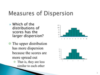
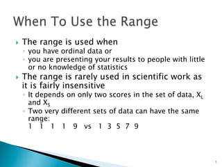
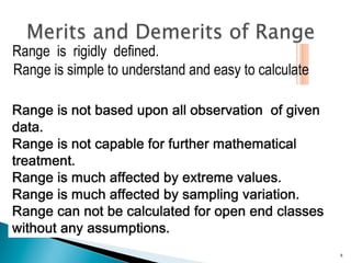
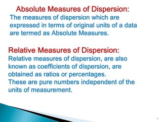
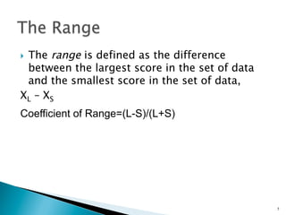
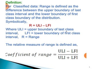
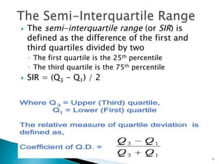
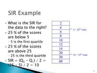
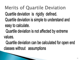
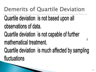
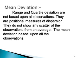
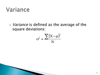
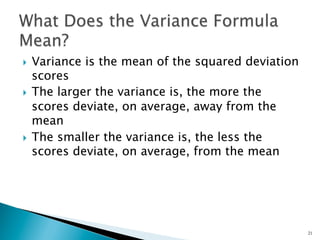
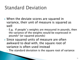
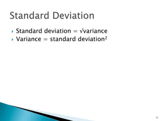
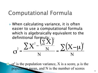
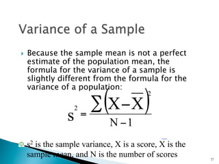
This document discusses several key concepts related to dispersion and variability in distributions: - Dispersion refers to how scattered or varied scores are around the central value. Greater dispersion means scores are less similar and more spread out. - Common measures of dispersion include the range, semi-interquartile range (SIR), variance, and standard deviation. Variance and standard deviation account for all scores rather than just the extremes. 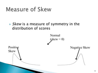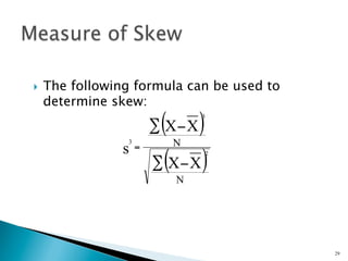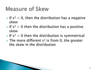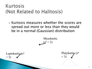- Other concepts discussed include skew, which measures symmetry, and kurtosis, which compares a distribution's spread to a normal distribution. These provide additional information about a distribution's shape beyond just dispersion.

1. } Dispersion or spread is the degree of the
scatter or variation of the variables about the
central value.
◦ The more similar the scores are to each other, the
lower the measure of dispersion will be
◦ The less similar the scores are to each other, the
higher the measure of dispersion will be
◦ In general, the more spread out a distribution is,
the larger the measure of dispersion will be
1

2. } Which of the 125
distributions of 100
scores has the
75
50
larger dispersion?
25
0
1 2 3 4 5 6 7 8 9 10
" The upper distribution
has more dispersion 125
100
because the scores are 75
50
more spread out 25
0
" That is, they are less
1 3 5 7 9
similar to each other
2

3. 3

4. } There are three main measures of dispersion:
◦ The range
◦ The semi-interquartile range (SIR)
◦ Variance / standard deviation
4

5. The range is defined as the difference
}
between the largest score in the set of data
and the smallest score in the set of data,
XL – XS
Coefficient of Range=(L-S)/(L+S)
5

6. 6

7. } The range is used when
◦ you have ordinal data or
◦ you are presenting your results to people with little
or no knowledge of statistics
} The range is rarely used in scientific work as
it is fairly insensitive
◦ It depends on only two scores in the set of data, XL
and XS
◦ Two very different sets of data can have the same
range:
1 1 1 1 9 vs 1 3 5 7 9
7

8. 8

9. } The semi-interquartile range (or SIR) is
defined as the difference of the first and
third quartiles divided by two
◦ The first quartile is the 25th percentile
◦ The third quartile is the 75th percentile
} SIR = (Q3 - Q1) / 2
9

10. } What is the SIR for 2
the data to the right? 4 ← 5 = 25th %tile
} 25 % of the scores 6
are below 5 8
◦ 5 is the first quartile 10
12
} 25 % of the scores
14
are above 25 20
◦ 25 is the third quartile
← 25 = 75th %tile
30
} SIR = (Q3 - Q1) / 2 = 60
(25 - 5) / 2 = 10
10

11. } The SIR is often used with skewed data as it is
insensitive to the extreme scores
11

12. 12

13. 13

14. 14

15. } Variance is defined as the average of the
square deviations:
∑ (X − µ)2
σ2 =
N
15

16. 16

17. 17

18. } First, it says to subtract the mean from each
of the scores
◦ This difference is called a deviate or a deviation
score
◦ The deviate tells us how far a given score is from
the typical, or average, score
◦ Thus, the deviate is a measure of dispersion for a
given score
18

19. } Why can’t we simply take the average of
the deviates? That is, why isn’t variance
defined as:
σ 2
≠
∑ (X − µ)
N
This is not the
formula for
variance!
19

20. } One of the definitions of the mean was that it
always made the sum of the scores minus the
mean equal to 0
} Thus, the average of the deviates must be 0
since the sum of the deviates must equal 0
} To avoid this problem, statisticians square
the deviate score prior to averaging them
◦ Squaring the deviate score makes all the squared
scores positive
20

21. } Variance is the mean of the squared deviation
scores
} The larger the variance is, the more the
scores deviate, on average, away from the
mean
} The smaller the variance is, the less the
scores deviate, on average, from the mean
21

22. } When the deviate scores are squared in
variance, their unit of measure is squared as
well
◦ E.g. If people’s weights are measured in pounds, then
the variance of the weights would be expressed in
pounds2 (or squared pounds)
} Since squared units of measure are often
awkward to deal with, the square root of
variance is often used instead
◦ The standard deviation is the square root of variance
22

23. } Standard deviation = √variance
} Variance = standard deviation2
23

24. } When calculating variance, it is often
easier to use a computational formula
which is algebraically equivalent to the
definitional formula: 2
∑X
2 (∑ X) 2
2
−
N ∑ (X −µ)
σ =
N
=
N
" σ2 is the population variance, X is a score, µ is the
population mean, and N is the number of scores 24

25. X X2 X-µ (X- µ)2
9 81 2 4
8 64 1 1
6 36 -1 1
5 25 -2 4
8 64 1 1
6 36 -1 1
Σ = 42 Σ = 306 Σ=0 Σ = 12
25

26. 2
(∑ X) 2
∑ (X −µ )
2
2
∑X −
N 2
σ =
N σ =
N
2
12
306 − 42 =
= 6 6
6 =2
306 − 294
=
6
12
=
6
=2
26

27. } Because the sample mean is not a perfect
estimate of the population mean, the
formula for the variance of a sample is
slightly different from the formula for the
variance of a population:
s
2
=
(
∑ X −X )2
N −1
" s2 is the sample variance, X is a score, X is the
sample mean, and N is the number of scores 27

28. } Skew is a measure of symmetry in the
distribution of scores
Normal
(skew = 0)
Positive Negative Skew
Skew
28

29. } The following formula can be used to
determine skew:
( )
∑ X− X
3
3 N
s =
∑ (X− X )
2
N
29

30. } If s3 < 0, then the distribution has a negative
skew
} If s3 > 0 then the distribution has a positive
skew
} If s3 = 0 then the distribution is symmetrical
} The more different s3 is from 0, the greater
the skew in the distribution
30

31. } Kurtosis measures whether the scores are
spread out more or less than they would
be in a normal (Gaussian) distribution
Mesokurtic
(s4 = 3)
Leptokurtic (s4 Platykurtic (s4
> 3) < 3)
31

32. } When the distribution is normally distributed,
its kurtosis equals 3 and it is said to be
mesokurtic
} When the distribution is less spread out than
normal, its kurtosis is greater than 3 and it is
said to be leptokurtic
} When the distribution is more spread out
than normal, its kurtosis is less than 3 and it
is said to be platykurtic
32