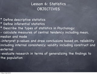
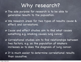
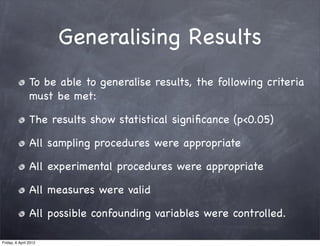
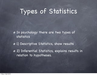
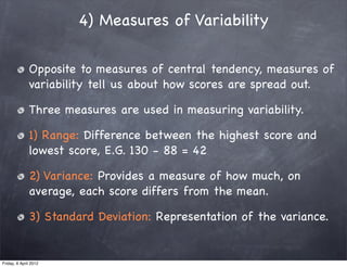
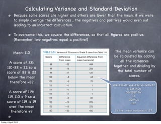
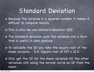
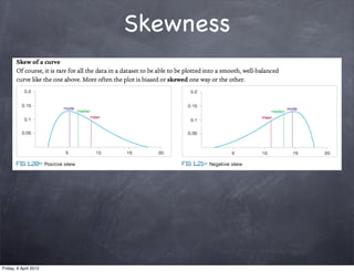
Lesson 6:

                       Research Methods
                               in Psychology
                          Stats and Graphs


Friday, 6 April 2012
Lesson 5
                       EXAM QUESTION


                        Taken from VCAA 2011 Mid Year Exam
Friday, 6 April 2012
Text


Friday, 6 April 2012
Lesson 6: Statistics
                          OBJECTIVES

* Define descriptive statistics 
* Define inferential statistics 
* Describe the types of statistics in Psychology:
- calculate measures of central tendency including mean,
median and mode
-interpret p-values and draw conclusions based on, reliability
including internal consistency; validity including construct and
external
-evaluate research in terms of generalizing the findings to
the population


Friday, 6 April 2012
Why research?
                 The sole purpose for research is to be able to
                 generalise results to the population.

                 We research areas for two types of results: cause &
                 effect, and correlations.

                 Cause and effect studies aim to find what causes
                 something e.g. smoking causes lung cancer

                 Correlational studies aim to find relationships between
                 two factors, e.g. as the population of smokers
                 increases so to does the diagnosis of lung cancer.

                 It is much easier to determine correlational results
                 than causative.
Friday, 6 April 2012
Generalising Results
                To be able to generalise results, the following criteria
                must be met:

                The results show statistical significance (p<0.05)

                All sampling procedures were appropriate

                All experimental procedures were appropriate

                All measures were valid

                All possible confounding variables were controlled.

Friday, 6 April 2012
Types of Statistics

                       In psychology there are two types of
                       statistics

                       1) Descriptive Statistics, show results

                       2) Inferential Statistics, explains results in
                       relation to hypotheses.


Friday, 6 April 2012
Descriptive Statistics

                       Includes the following:

                       1) Organising raw data into clear tables

                       2) Representing the data in graphs

                       3) Measures of Central Tendency

                       4) Measures of Variability


Friday, 6 April 2012
1)Organising Raw Data
                Frequency tables are the most common form of organising raw
                data.

                For example, Julie rolled a die 80 times and recorded the number
                shown on each throw: 1, 3, 6, 5, 2, 1, 6, 1, 5, 2, 1, 2, 5, 4, 3, 6, 5,
                2, 3, 4, 1, 4, 3, 2, 5, 1, 6, 2, 3, 1, 5, 5, 2, 3, 5, 4, 1, 3, 5, 3, 6, 3, 1,
                6, 6, 3, 3, 4, 3, 3, 6, 3, 1, 3, 4, 6, 2, 4, 6, 3, 4, 5, 4, 6, 2, 3, 4, 5, 5,
                4, 2, 1, 5, 4, 5, 6, 1, 6, 2, 5. - This is raw data.

          To organise the data, a frequency
             table can be used. Here the
          amount of times the number was
          rolled (frequency) is listed beside
            the dice number. In frequency
              tables we also include the
            percentage of that frequency.


Friday, 6 April 2012
Calculating the
                              percentage

                       Number of times score occurs DIVIDED BY
                       Total number of scores in data set
                       MULTIPLIED BY 100

                       E.G. The percentage of rolling a 6 would be:

                          13/80 = 0.1625 x 100 = 16.25%


Friday, 6 April 2012
2) Representing the data

                            Histogram

                                  Frequency
                                   Polygon

                              Pie Chart


Friday, 6 April 2012
The normal distribution
                                “Bell Curve”
                When one variable is continuous (meaning that it can have any
                value within a certain range) such as age in months or IQ, we
                can express the data as a line graph.

                For example, a teacher sets a group classwork activity and wants
                to find out the group size that is most efficient.


Friday, 6 April 2012
When data is presented in a line graph, psychologists
                hope that it forms a normal curve.

                This enables statistical procedures to be applied
                without further manipulation of the data.


Friday, 6 April 2012
3) Measures of Central Tendency
                         (Measures in the Bell Curve)
                Tells us how the data are clustered near the central
                point of the dataset.

                There are three measures of central tendency
                1) Mean - average of all the scores (calculated by
                adding up all the scores and dividing that total by the
                number of scores)
                2) Median - the score that occurs exactly halfway
                between the lowest and the highest score.
                3) Mode - the most commonly occurring score in the
                dataset.

Friday, 6 April 2012
4) Measures of Variability

              Opposite to measures of central tendency, measures of
              variability tell us about how scores are spread out.

              Three measures are used in measuring variability.

              1) Range: Difference between the highest score and
              lowest score, E.G. 130 - 88 = 42

              2) Variance: Provides a measure of how much, on
              average, each score differs from the mean.

              3) Standard Deviation: Representation of the variance.


Friday, 6 April 2012
Calculating Variance and Standard Deviation
               Because some scores are higher and others are lower than the mean, if we were
               to simply average the differences , the negatives and positives would even out
               leading to an incorrect calculation.

               To overcome this, we square the differences, so that all figures are positive.
               (Remember two negatives equal a positive!)


              Mean: 110                                                   The mean variance can
                                                                         be calculated by adding
         A score of 88:                                                      all the variances
       110-88 = 22 so a                                                  together and dividing by
       score of 88 is 22                                                   the total number of
        below the mean                                                             scores.
         therefore -22
                                                                         484+256+121+64+25+1+1+1+81+22
                                                                                  5+225+400
         A score of 119:                                                          DIVIDED BY
        119-110 = 9 so a                                                               12
                                                                                    EQUALS
       score of 119 is 19                                                             157
         over the mean
          therefore +9                                                    So the mean variance is 157.


Friday, 6 April 2012
Standard Deviation
               Because the variance is a squared number, it makes it
               difficult to compare results.

               This is why we use standard deviation (SD).

               The standard deviation puts the variance into a form
               that is useful in data analyse.

               To calculate the SD you take the square root of the
               mean variance. E.G. Square root of 157 = 12.5

               Only get the SD for the mean variance! All the other
               variances still along the normal curve as SD from the
               mean.
Friday, 6 April 2012
Skewness


Friday, 6 April 2012
Inferential Statistics
                Inferential Statistics are used once the descriptive
                statistics have identified there is a difference
                (variation) from the mean.

                What next is to determine if this difference or
                variance is significant, or is it just due to chance.

                Inferential tests give a probability that the difference
                is caused by chance.

                  This is expressed as a p value.

                Generally the lower the p value the better, however
                p<0.05 (that is 5 times in 100 or 5% of the time it is
                due to chance) is widely accepted.
Friday, 6 April 2012
p = 0.03 means there are 3 chances in 100 (3%)
      that this difference would be achieved by chance
                            alone.

  If the level of significance is p<0.05 then these
results can be said to be statistically significant as it
                 is less then (<) 0.05

              If the p value = 0.3 then the results are not
                 significant as 0.3 is greater then 0.05.


Friday, 6 April 2012
Complete ‘INVESTIGATE 1.6’ p 24 of textbook


Friday, 6 April 2012
Measures of relationship
               Correlational studies intend to establish the strength
               and direction of any relationship between two
               variables.

               Correlation: A statistical measure of how much two
               variables are related.

               Positive Correlation: Where the two variables change in
               the same direction. As one increases so to does the
               other.

               Negative Correlation: Where the two variables change
               in the opposite direction. As one increases the other
               decreases.
Friday, 6 April 2012
Strength in correlation
                The strength of a correlation can be calculated using
                the correlation coefficient (r).

                The (+) or (-) sign before the coefficient indicates if it
                is a positive or negative correlation.

                The number is the coefficient, the higher the number
                the stronger the relationship.


Friday, 6 April 2012
Scatter Plots


Friday, 6 April 2012
Determine the strength (strong or weak) and
          direction (positive or negative) of the following
                             correlations:
                              r=-   0.74
                              r=+   1.00
                              r=+   0.23
                              r=-   0.15


Friday, 6 April 2012

Rm psych stats & graphs

  • 1.
    Lesson 6: Research Methods in Psychology Stats and Graphs Friday, 6 April 2012
  • 2.
    Lesson 5 EXAM QUESTION Taken from VCAA 2011 Mid Year Exam Friday, 6 April 2012
  • 3.
  • 4.
    Lesson 6: Statistics OBJECTIVES * Define descriptive statistics  * Define inferential statistics  * Describe the types of statistics in Psychology: - calculate measures of central tendency including mean, median and mode -interpret p-values and draw conclusions based on, reliability including internal consistency; validity including construct and external -evaluate research in terms of generalizing the findings to the population   Friday, 6 April 2012
  • 5.
    Why research? The sole purpose for research is to be able to generalise results to the population. We research areas for two types of results: cause & effect, and correlations. Cause and effect studies aim to find what causes something e.g. smoking causes lung cancer Correlational studies aim to find relationships between two factors, e.g. as the population of smokers increases so to does the diagnosis of lung cancer. It is much easier to determine correlational results than causative. Friday, 6 April 2012
  • 6.
    Generalising Results To be able to generalise results, the following criteria must be met: The results show statistical significance (p<0.05) All sampling procedures were appropriate All experimental procedures were appropriate All measures were valid All possible confounding variables were controlled. Friday, 6 April 2012
  • 7.
    Types of Statistics In psychology there are two types of statistics 1) Descriptive Statistics, show results 2) Inferential Statistics, explains results in relation to hypotheses. Friday, 6 April 2012
  • 8.
    Descriptive Statistics Includes the following: 1) Organising raw data into clear tables 2) Representing the data in graphs 3) Measures of Central Tendency 4) Measures of Variability Friday, 6 April 2012
  • 9.
    1)Organising Raw Data Frequency tables are the most common form of organising raw data. For example, Julie rolled a die 80 times and recorded the number shown on each throw: 1, 3, 6, 5, 2, 1, 6, 1, 5, 2, 1, 2, 5, 4, 3, 6, 5, 2, 3, 4, 1, 4, 3, 2, 5, 1, 6, 2, 3, 1, 5, 5, 2, 3, 5, 4, 1, 3, 5, 3, 6, 3, 1, 6, 6, 3, 3, 4, 3, 3, 6, 3, 1, 3, 4, 6, 2, 4, 6, 3, 4, 5, 4, 6, 2, 3, 4, 5, 5, 4, 2, 1, 5, 4, 5, 6, 1, 6, 2, 5. - This is raw data. To organise the data, a frequency table can be used. Here the amount of times the number was rolled (frequency) is listed beside the dice number. In frequency tables we also include the percentage of that frequency. Friday, 6 April 2012
  • 10.
    Calculating the percentage Number of times score occurs DIVIDED BY Total number of scores in data set MULTIPLIED BY 100 E.G. The percentage of rolling a 6 would be: 13/80 = 0.1625 x 100 = 16.25% Friday, 6 April 2012
  • 11.
    2) Representing thedata Histogram Frequency Polygon Pie Chart Friday, 6 April 2012
  • 12.
    The normal distribution “Bell Curve” When one variable is continuous (meaning that it can have any value within a certain range) such as age in months or IQ, we can express the data as a line graph. For example, a teacher sets a group classwork activity and wants to find out the group size that is most efficient. Friday, 6 April 2012
  • 13.
    When data ispresented in a line graph, psychologists hope that it forms a normal curve. This enables statistical procedures to be applied without further manipulation of the data. Friday, 6 April 2012
  • 14.
    3) Measures ofCentral Tendency (Measures in the Bell Curve) Tells us how the data are clustered near the central point of the dataset. There are three measures of central tendency 1) Mean - average of all the scores (calculated by adding up all the scores and dividing that total by the number of scores) 2) Median - the score that occurs exactly halfway between the lowest and the highest score. 3) Mode - the most commonly occurring score in the dataset. Friday, 6 April 2012
  • 15.
  • 16.
    4) Measures ofVariability Opposite to measures of central tendency, measures of variability tell us about how scores are spread out. Three measures are used in measuring variability. 1) Range: Difference between the highest score and lowest score, E.G. 130 - 88 = 42 2) Variance: Provides a measure of how much, on average, each score differs from the mean. 3) Standard Deviation: Representation of the variance. Friday, 6 April 2012
  • 17.
    Calculating Variance andStandard Deviation Because some scores are higher and others are lower than the mean, if we were to simply average the differences , the negatives and positives would even out leading to an incorrect calculation. To overcome this, we square the differences, so that all figures are positive. (Remember two negatives equal a positive!) Mean: 110 The mean variance can be calculated by adding A score of 88: all the variances 110-88 = 22 so a together and dividing by score of 88 is 22 the total number of below the mean scores. therefore -22 484+256+121+64+25+1+1+1+81+22 5+225+400 A score of 119: DIVIDED BY 119-110 = 9 so a 12 EQUALS score of 119 is 19 157 over the mean therefore +9 So the mean variance is 157. Friday, 6 April 2012
  • 18.
    Standard Deviation Because the variance is a squared number, it makes it difficult to compare results. This is why we use standard deviation (SD). The standard deviation puts the variance into a form that is useful in data analyse. To calculate the SD you take the square root of the mean variance. E.G. Square root of 157 = 12.5 Only get the SD for the mean variance! All the other variances still along the normal curve as SD from the mean. Friday, 6 April 2012
  • 19.
  • 20.
  • 21.
    Inferential Statistics Inferential Statistics are used once the descriptive statistics have identified there is a difference (variation) from the mean. What next is to determine if this difference or variance is significant, or is it just due to chance. Inferential tests give a probability that the difference is caused by chance. This is expressed as a p value. Generally the lower the p value the better, however p<0.05 (that is 5 times in 100 or 5% of the time it is due to chance) is widely accepted. Friday, 6 April 2012
  • 22.
    p = 0.03means there are 3 chances in 100 (3%) that this difference would be achieved by chance alone. If the level of significance is p<0.05 then these results can be said to be statistically significant as it is less then (<) 0.05 If the p value = 0.3 then the results are not significant as 0.3 is greater then 0.05. Friday, 6 April 2012
  • 23.
    Complete ‘INVESTIGATE 1.6’p 24 of textbook Friday, 6 April 2012
  • 24.
    Measures of relationship Correlational studies intend to establish the strength and direction of any relationship between two variables. Correlation: A statistical measure of how much two variables are related. Positive Correlation: Where the two variables change in the same direction. As one increases so to does the other. Negative Correlation: Where the two variables change in the opposite direction. As one increases the other decreases. Friday, 6 April 2012
  • 25.
    Strength in correlation The strength of a correlation can be calculated using the correlation coefficient (r). The (+) or (-) sign before the coefficient indicates if it is a positive or negative correlation. The number is the coefficient, the higher the number the stronger the relationship. Friday, 6 April 2012
  • 26.
  • 27.
    Determine the strength(strong or weak) and direction (positive or negative) of the following correlations: r=- 0.74 r=+ 1.00 r=+ 0.23 r=- 0.15 Friday, 6 April 2012