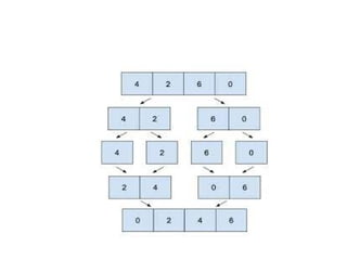
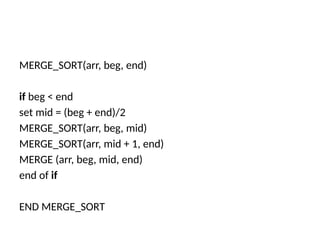
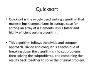
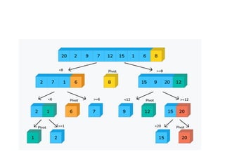
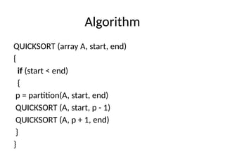
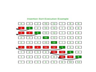
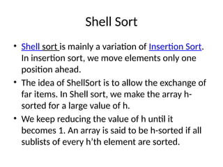
The document provides an in-depth overview of various sorting algorithms, including merge sort, quicksort, insertion sort, shell sort, and radix sort, highlighting their techniques and efficiency. It also covers hashing concepts, including hash functions, collision handling through methods like separate chaining and open addressing, and the rehashing process. Additionally, it discusses applications of these algorithms in areas such as symbol tables, caching, and databases.

1. UNIT V
SORTING AND HASHING
TECHNIQUES

2. Sorting
• Sorting refers to arranging data in a particular
format. Sorting algorithm specifies the way to
arrange data in a particular order. Most
common orders are in numerical or
lexicographical order.
• The importance of sorting lies in the fact that
data searching can be optimized to a very high
level, if data is stored in a sorted manner.

3. Merge sort
• Merge sort is defined as a sorting algorithm
that works by dividing an array into smaller
subarrays, sorting each subarray, and then
merging the sorted subarrays back together to
form the final sorted array.

5. MERGE_SORT(arr, beg, end)
if beg < end
set mid = (beg + end)/2
MERGE_SORT(arr, beg, mid)
MERGE_SORT(arr, mid + 1, end)
MERGE (arr, beg, mid, end)
end of if
END MERGE_SORT

6. Quicksort
• Quicksort is the widely used sorting algorithm that
makes n log n comparisons in average case for
sorting an array of n elements. It is a faster and
highly efficient sorting algorithm.
• This algorithm follows the divide and conquer
approach. Divide and conquer is a technique of
breaking down the algorithms into subproblems,
then solving the subproblems, and combining the
results back together to solve the original problem.

7. • Divide: In Divide, first pick a pivot element.
After that, partition or rearrange the array into
two sub-arrays such that each element in the
left sub-array is less than or equal to the pivot
element and each element in the right sub-
array is larger than the pivot element.
• Conquer: Recursively, sort two subarrays with
Quicksort.
• Combine: Combine the already sorted array.

9. Algorithm
QUICKSORT (array A, start, end)
{
if (start < end)
{
p = partition(A, start, end)
QUICKSORT (A, start, p - 1)
QUICKSORT (A, p + 1, end)
}
}

10. Insertion sort
• Insertion sort is a simple sorting algorithm
that works similar to the way you sort playing
cards in your hands. The array is virtually split
into a sorted and an unsorted part. Values
from the unsorted part are picked and placed
at the correct position in the sorted part.

12. Shell Sort
• Shell sort is mainly a variation of Insertion Sort.
In insertion sort, we move elements only one
position ahead.
• The idea of ShellSort is to allow the exchange of
far items. In Shell sort, we make the array h-
sorted for a large value of h.
• We keep reducing the value of h until it
becomes 1. An array is said to be h-sorted if all
sublists of every h’th element are sorted.

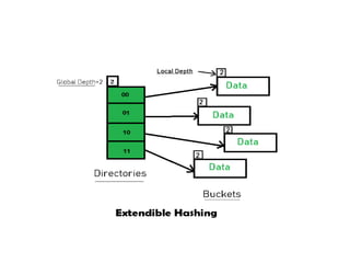
13. • PROCEDURE SHELL_SORT(ARRAY, N)
WHILE GAP < LENGTH(ARRAY) /3 :
GAP = ( INTERVAL * 3 ) + 1
END WHILE LOOP
WHILE GAP > 0 :
FOR (OUTER = GAP; OUTER < LENGTH(ARRAY); OUTER++):
INSERTION_VALUE = ARRAY[OUTER]
INNER = OUTER;
WHILE INNER > GAP-1 AND ARRAY[INNER – GAP] >=
INSERTION_VALUE:
ARRAY[INNER] = ARRAY[INNER – GAP]
INNER = INNER – GAP
END WHILE LOOP
ARRAY[INNER] = INSERTION_VALUE
END FOR LOOP

15. Radix sort
• Radix Sort is a linear sorting algorithm that
sorts elements by processing them digit by
digit. It is an efficient sorting algorithm for
integers or strings with fixed-size keys.
• Radix Sort distributes the elements into
buckets based on each digit’s value.

17. • Hashing is the process of generating a value from a
text or a list of numbers using a mathematical function
known as a hash function.
• A Hash Function is a function that converts a given
numeric or alphanumeric key to a small practical
integer value. The mapped integer value is used as an
index in the hash table. In simple terms, a hash
function maps a significant number or string to a small
integer that can be used as the index in the hash table.

18. • The pair is of the form (key, value), where for a given key, one can find a
value using some kind of a “function” that maps keys to values.
• A good hash function should have the following properties:
• Efficiently computable.
• Should uniformly distribute the keys (Each table position is equally likely
for each.
• Should minimize collisions.
• Should have a low load factor(number of items in the table divided by the
size of the table).
• Complexity of calculating hash value using the hash function
• Time complexity: O(n)
• Space complexity: O(1)

20. Collision
• Collision in Hashing
• In this, the hash function is used to find the
index of the array. The hash value is used to
create an index for the key in the hash table.
The hash function may return the same hash
value for two or more keys. When two or more
keys have the same hash value, a collision
happens. To handle this collision, we use
collision resolution techniques.

21. Collision Resolution Techniques
• There are two types of collision resolution techniques.
• Separate chaining (open hashing)
• Open addressing (closed hashing)
• Separate chaining: This method involves making a linked list out of
the slot where the collision happened, then adding the new key to
the list. Separate chaining is the term used to describe how this
connected list of slots resembles a chain. It is more frequently
utilized when we are unsure of the number of keys to add or
remove.
• Time complexity
• Its worst-case complexity for searching is o(n).
• Its worst-case complexity for deletion is o(n).

22. • Open addressing: To prevent collisions in the hashing
table open, addressing is employed as a collision-
resolution technique. No key is kept anywhere else
besides the hash table. As a result, the hash table’s size
is never equal to or less than the number of keys.
Additionally known as closed hashing.
• The following techniques are used in open addressing:
• Linear probing
• Quadratic probing
• Double hashing

23. Linear Probing
• In linear probing, the hash table is searched
sequentially that starts from the original
location of the hash. If in case the location
that we get is already occupied, then we check
for the next location.
• The function used for rehashing is as follows:
rehash(key) = (n+1)%table-size.

25. Applications
• Symbol tables: Linear probing is commonly used in symbol tables,
which are used in compilers and interpreters to store variables and
their associated values. Since symbol tables can grow dynamically,
linear probing can be used to handle collisions and ensure that
variables are stored efficiently.
• Caching: Linear probing can be used in caching systems to store
frequently accessed data in memory. When a cache miss occurs, the
data can be loaded into the cache using linear probing, and when a
collision occurs, the next available slot in the cache can be used to
store the data.
• Databases: Linear probing can be used in databases to store records
and their associated keys. When a collision occurs, linear probing
can be used to find the next available slot to store the record.

26. Separate Chaining
• The idea behind separate chaining is to implement
the array as a linked list called a chain. Separate
chaining is one of the most popular and commonly
used techniques in order to handle collisions.
• The linked list data structure is used to implement
this technique. So what happens is, when multiple
elements are hashed into the same slot index,
then these elements are inserted into a singly-
linked list which is known as a chain.

28. Open Addressing
• In Open Addressing, all elements are stored in
the hash table itself. So at any point, the size
of the table must be greater than or equal to
the total number of keys.
• This approach is also known as closed
hashing. This entire procedure is based upon
probing. We will understand the types of
probing ahead:

29. • Insert(k): Keep probing until an empty slot is
found. Once an empty slot is found, insert k.
• Search(k): Keep probing until the slot’s key
doesn’t become equal to k or an empty slot is
reached.
• Delete(k): Delete operation is interesting. If
we simply delete a key, then the search may
fail. So slots of deleted keys are marked
specially as “deleted”.

30. Rehashing
• Rehashing is the process of recalculating the
hashcode of previously-stored entries (Key-
Value pairs) in order to shift them to a larger
size hashmap when the threshold is
reached/crossed,
• When the number of elements in a hash map
reaches the maximum threshold value, it is
rehashed.

32. How Rehashing is done?
Rehashing can be done as follows:
• For each addition of a new entry to the map, check the
load factor.
• If it’s greater than its pre-defined value (or default
value of 0.75 if not given), then Rehash.
• For Rehash, make a new array of double the previous
size and make it the new bucketarray.
• Then traverse to each element in the old bucketArray
and call the insert() for each so as to insert it into the
new larger bucket array.

33. Extendible Hashing
• Extendible Hashing is a dynamic hashing method wherein
directories, and buckets are used to hash data. It is an
aggressively flexible method in which the hash function
also experiences dynamic changes.
• Main features of Extendible Hashing: The main features
in this hashing technique are:
• Directories: The directories store addresses of the buckets
in pointers. An id is assigned to each directory which may
change each time when Directory Expansion takes place.
• Buckets: The buckets are used to hash the actual data.