Scilab

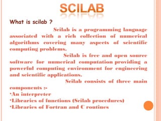
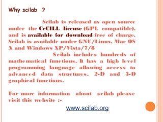
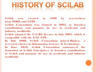
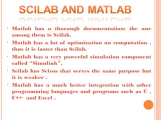
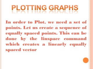
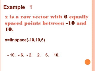
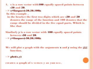
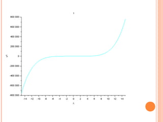
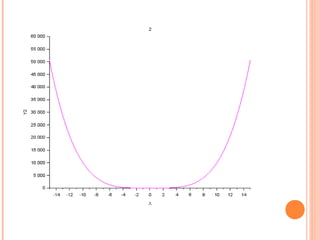
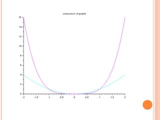
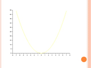
C. K. PITHAWALA COLLEGE OF
ENGINEERING AND
TECHNOLOGY

NAME
ROLL NO.
1. PRAJAPATI ABHAY
173
2. CHINTAN BHATT
128
3. RANA SRUSHTI
175
4. MARSONIYA HEM
148
5. AMAN PATEL
152

•Scilab
•History of scilab
•Scilab and matlab
•Plotting graphs
•Comparison of graphs
•Shifting of graphs
objectives

What is scilab ?
Scilab is a programming language
associated with a rich collection of numerical
algorithms covering many aspects of scientific
computing problems.
Scilab is free and open source
software for numerical computation providing a
powerful computing environment for engineering
and scientific applications.
Scilab consists of three main
components :-
•An interpreter
•Libraries of functions (Scilab procedures)
•Libraries of Fortran and C routines

Why scilab ?
Scilab is released as open source
under the CeCILL license (GPL compatible),
and is available for download free of charge.
Scilab is available under GNU/Linux, Mac OS
X and Windows XP/Vista/7/8
Scilab includes hundreds of
mathematical functions. It has a high level
programming language allowing access to
advanced data structures, 2-D and 3-D
graphical functions.
For more information about scilab please
visit this website :-
www.scilab.org

Scilab was created in 1990 by researchers
from INRIA and ENPC.
Scilab Consortium was formed in 2003, to broaden
contributions and promote its use in academia and
industry worldwide.
Scilab adopted the CeCILL license in July 2004, which is
compatible with the GNU GPL.
In July 2008, Scilab Consortium joined Digiteo, a
research cluster in Information Science & Technology.
In June 2010, Scilab Consortium announced the
formation of Scilab Enterprises to broaden contributions
to Scilab and promote its use in academis and industry
worldwide.

• Matlab has a thorough documentation; the one
among them is Scilab.
• Matlab has a lot of optimization on computation ,
thus it is faster than Scilab.
• Matlab has a very powerful simulation component
called “Simulink”.
• Scilab has Scicos that serves the same purpose but
it is weaker .
• Matlab has a much better integration with other
programming languages and programs such as C ,
C++ and Excel .

•The graphics components of Scilab is weak
i.e. it has less functions .
•Most important and the key advantage of
Scilab is that it can be easily available at
FREE of cost . It certainly outweighs its
deficiencies. It is remarked that Scilab is
more than enough for casual and educational
purposes.

In order to Plot, we need a set of
points. Let us create a sequence of
equally spaced points. This can be
done by the linspace command
which creates a linearly equally
spaced vector

x is a row vector with 6 equally
spaced points between -10 and
10.
x=linspace(-10,10,6)
- 10. - 6. - 2. 2. 6. 10.
Example 1

1. x is a row vector with100 equally spaced points between
-50 and 50.
‐‐> x=linspace(-50,50,100);
In this example ,
in the bracket the first two digits which are -50 and 50
denotes the range of the function and 100 denotes that the
range should be divided in the five equal parts. Which is
like that
Similarly y is a row vector with 100 equally spaced points
between -30 and 20.
‐‐> y=linspace(-30,20,100);

We will plot a graph with the arguments x and y using the plot
function.

‐‐> plot(x,y)

creates a graph of x verses y as you see.

For plotting 2d graphs we take a example :--
2. x is a row vector with 50 equally spaced points between
1 and 100.
---> x=linspace(1,100,50);
and y is a row vector with 50 eqally spaced points between
-10 and
10.
---> y=linspace(-10,10,50);
Now for the 2d graph the function is
Plot2d(x,y,style=2)plot2d command plot a graph of x verses y as you see.
Notice that there is a third argument called style and
this argument is optional. It is used to customize the appearance of
the plot.
For positive values of style, the curve is a plain line with different
colors, like dark blue is given 2 in our case. The default value of style
is 1. For different negative and positive values, the appearance of the
graph differs.

To configure labels to the axis and title of the plot we can
use the commands
--> title(“name of title")
-->xlabel("X") X= name of x-axis
-->ylabel("Y") Y= name of y-axis

You will see that the graph has been labeled X to the x
axis, Y to the y axis and title of the graph is name of title.

DIFFERENT STYLES :-
 Style 1 :- Black
 Style 2 :- Dark Blue
 Style 3 :- Green
 Style 4 :- Light Blue
 Style 5 :- Red
 Style 6:- Pink
 Style 7 :- Yellow
 Style 8 :- White
 Style 9 :- Blackish Blue
Similarly, value of Style can be given as
negative values but in that instead of color it will
give different types of symbols .

If we take negative value of style then the graph is like
that :-

CLF AND CLEAR COMMANDS:-
The clf() function will clear the graphic window.
‐‐> clf()
It is useful while plotting different graph on the
same graphic window.
While ,the clear command is used to clear the
display i.e. it will clear the values of x and y
displayed on the screen.

COMPARESION OF TWO DIFFERENT
GRAPHS
For example,
‐‐> x=linspace(-15,15,80);
‐‐> y1=x^5;
Note that here ‘^’ symbol is denoted for power
Then, y2=x^4;
-->plot(x,y1, style=4)---------------------(1)
-->plot(x,y2,style=6)----------------------(2)
Now you can see the graphs below respectively.

SHIFTING OF GRAPH
Now, taking example we can present shifting of
graphs
x=linspace(-7,7,60);
y1=x^2;
y2=(x-3)^2;
plot2d(x,y1,style=7)--------------(1)
plot2d(x,y2,style=6)---------------(2)

Scilab

More Related Content

What's hot

Similar to Scilab

Recently uploaded

Scilab