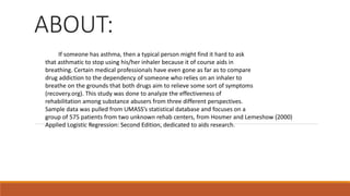
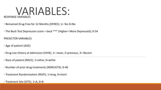
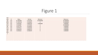
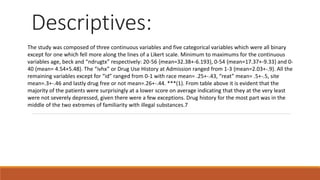
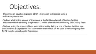
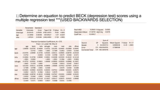
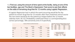
Effectiveness Of Rehabilitation
Facilities
ABOUT:
If someone has asthma, then a typical person might find it hard to ask
that asthmatic to stop using his/her inhaler because it of course aids in
breathing. Certain medical professionals have even gone as far as to compare
drug addiction to the dependency of someone who relies on an inhaler to
breathe on the grounds that both drugs aim to relieve some sort of symptoms
(recovery.org). This study was done to analyze the effectiveness of
rehabilitation among substance abusers from three different perspectives.
Sample data was pulled from UMASS’s statistical database and focuses on a
group of 575 patients from two unknown rehab centers, from Hosmer and Lemeshow (2000)
Applied Logistic Regression: Second Edition, dedicated to aids research.
VARIABLES:RESPONSE VARIABLES
◦ Remained Drug Free for 12 Months (DFREE); 1= Yes 0=No
◦ The Beck Test Depression score = beck *** (Higher= More Depressed); 0-54
PREDICTOR VARIABLES
◦ Age of patient (AGE)
◦ Drug Use History at Admission (IVHX); 1= never, 2=previous, 3= Recent
◦ Race of patient (RACE); 1=other, 0=white
◦ Number of prior drug treatments (NDRUGTX); 0-40
◦ Treatment Randomization (REAT); 1=long, 0=short
◦ Treatment Site (SITE); 1=A, 0=B
Figure 1
Vari
able N Mean Std Dev Minimum Maximum
age
beck
ivhx
ndru
gtx
race
reat
site
dfre
e
575
575
575
575
575
575
575
575
32.3826087
17.3674278
2.0347826
4.5426087
0.2521739
0.4973913
0.3043478
0.2556522
6.1931493
9.3329625
0.9003526
5.4754291
0.4346387
0.5004285
0.4605313
0.4366070
20.0000000
0
1.0000000
0
0
0
0
0
56.0000000
54.0000000
3.0000000
40.0000000
1.0000000
1.0000000
1.0000000
1.0000000
Figure 2
dfree Frequency Percent
Cumulative
Frequency
Cumulative
Percent
0 428 74.43 428 74.43
1 147 25.57 575 100.00
Descriptives:
The study was composed of three continuous variables and five categorical variables which were all binary
except for one which fell more along the lines of a Likert scale. Minimum to maximums for the continuous
variables age, beck and “ndrugtx” respectively: 20-56 {mean=32.38+-6.193}, 0-54 {mean=17.37+-9.33} and 0-
40 {mean= 4.54+5.48}. The “ivhx” or Drug Use History at Admission ranged from 1-3 {mean=2.03+-.9}. All the
remaining variables except for “id” ranged from 0-1 with race mean= .25+-.43, “reat” mean= .5+-.5, site
mean=.3+-.46 and lastly drug free or not mean=.26+-.44. ***(1). From table above it is evident that the
majority of the patients were surprisingly at a lower score on average indicating that they at the very least
were not severely depressed, given there were a few exceptions. Drug history for the most part was in the
middle of the two extremes of familiarity with illegal substances.7
Objectives:
•Determine an equation to predict BECK (depression test) scores using a
multiple regression test
•Find out whether the amount of time spent at the facility and which of the two facilities
affect the odds of remaining drug free for 12 moths after rehabilitation using 2x2 Chi-Sq. Tests
•Find out, using the amount of time spent at the facility, being at one of the two facilities, age
and The Beck’s Depression Test score to see their effects on the odds of remaining drug-free
for 12 months using Logistic Regression.
1) Determine an equation to predict BECK (depression test) scores using a
multiple regression test ***(USED BACKWARDS SELECTION)
Variable
Parameter
Estimate
Standard
Error Type II SS F Value Pr > F
Intercept 18.36143 2.05505 6766.16553 79.83 <.0001
age -0.14858 0.06598 429.84617 5.07 0.0247
ivhx 1.87614 0.45384 1448.44092 17.09 <.0001
Pearson Correlation Coefficients, N = 575
Prob > |r| under H0: Rho=0
age beck ivhx ndrugtx race reat site dfree
age 1.00000 -0.03705
0.3752
0.34004
<.0001
0.19752
<.0001
0.01393
0.7389
-0.04465
0.2852
-0.02868
0.4924
0.04945
0.2364
beck -0.03705
0.3752
1.00000 0.14746
0.0004
0.05925
0.1559
0.00111
0.9788
0.00965
0.8175
-0.08749
0.0360
-0.03318
0.4271
ivhx 0.34004
<.0001
0.14746
0.0004
1.00000 0.30821
<.0001
-0.20498
<.0001
-0.05393
0.1966
-0.18103
<.0001
-0.15118
0.0003
ndrugtx 0.19752
<.0001
0.05925
0.1559
0.30821
<.0001
1.00000 -0.09859
0.0180
-0.00203
0.9613
-0.09808
0.0187
-0.13027
0.0017
race 0.01393
0.7389
0.00111
0.9788
-0.20498
<.0001
-0.09859
0.0180
1.00000 0.07912
0.0579
-0.07947
0.0569
0.09117
0.0288
reat -0.04465
0.2852
0.00965
0.8175
-0.05393
0.1966
-0.00203
0.9613
0.07912
0.0579
1.00000 -0.02301
0.5819
0.09475
0.0231
site -0.02868
0.4924
-0.08749
0.0360
-0.18103
<.0001
-0.09808
0.0187
-0.07947
0.0569
-0.02301
0.5819
1.00000 0.05425
0.1940
dfree 0.04945
0.2364
-0.03318
0.4271
-0.15118
0.0003
-0.13027
0.0017
0.09117
0.0288
0.09475
0.0231
0.05425
0.1940
1.00000
Root MSE 9.20633 R-Square 0.0303
Dependent Mean 17.36743 Adj R-Sq 0.0270
Coeff Var 53.00917
Source DF
Sum of
Squares Mean Square F Value Pr > F
Model 3 26.4024713 8.8008238 11.45 <.0001
Error 571 438.9018765 0.7686548
Corrected Total 574 465.3043478
•2) Find out, using the amount of time spent at the facility, being at one of the
two facilities, age and The Beck’s Depression Test score to see their effects
on the odds of remaining drug-free for 12 months using Logistic Regression.
◦ A Logistic Regression test in which the event occurring would be for the
patient to remain drug-free for 12 months after their treatment and of course
the non-event would be for the patient to relapse before the 12 month
sobriety mark. At a 0.7 Probability cutoff level there is a corresponding 65.6
correct percentage, 78% sensitivity and 27.9 specificity.
Analysis of Maximum Likelihood Estimates
Parameter DF Estimate
Standard
Error
Wald
Chi-Square Pr > ChiSq
Intercept 1 1.9251 0.5711 11.3619 0.0007
age 1 -0.0199 0.0154 1.6763 0.1954
beck 1 0.00687 0.0105 0.4298 0.5121
site 1 -0.2721 0.2059 1.7470 0.1863
reat 1 -0.4569 0.1941 5.5431 0.0186
Odds Ratio Estimates and Wald Confidence Intervals
Effect Unit Estimate 95% Confidence Limits
age 1.0000 0.980 0.951 1.010
beck 1.0000 1.007 0.986 1.028
site 1.0000 0.762 0.509 1.140
reat 1.0000 0.633 0.433 0.926
Hosmer and Lemeshow
Goodness-of-Fit Test
Chi-Square DF Pr > ChiSq
15.5261 8 0.0497
Conclusion:
The predictor equation in which I used age and drug-use history
levels to estimate a Beck’s Test Depression score ranging from 0-54.
Residuals look as they should ideally although the coefficient of
determination, R-squared indicates that around 3.03% of the variation
about the line could be explained by using age and past drug history to
explain the depression test scores. Another test was ran on the same
data using Logistic Regression to determine the odds of a patient
remaining sober for 12 months after being released from rehab.
Results indicated that the older one was the less likely they were to
make it 12 months sober. Similarly, those who stayed at site A for the
longer time period greatly decreased their odds of making it a year
without drug abuse.
Limitations/
Recommendations
While I was limited to only being able to utilize 3 continuous variables the overstock in categorical variables
allowed for more odds-based tests. As a result the R-square value for my predictive equation model was low
due to the lack of continuous variables.

sas final presentation delgado (1)

  • 1.
  • 2.
    ABOUT: If someone hasasthma, then a typical person might find it hard to ask that asthmatic to stop using his/her inhaler because it of course aids in breathing. Certain medical professionals have even gone as far as to compare drug addiction to the dependency of someone who relies on an inhaler to breathe on the grounds that both drugs aim to relieve some sort of symptoms (recovery.org). This study was done to analyze the effectiveness of rehabilitation among substance abusers from three different perspectives. Sample data was pulled from UMASS’s statistical database and focuses on a group of 575 patients from two unknown rehab centers, from Hosmer and Lemeshow (2000) Applied Logistic Regression: Second Edition, dedicated to aids research.
  • 3.
    VARIABLES:RESPONSE VARIABLES ◦ RemainedDrug Free for 12 Months (DFREE); 1= Yes 0=No ◦ The Beck Test Depression score = beck *** (Higher= More Depressed); 0-54 PREDICTOR VARIABLES ◦ Age of patient (AGE) ◦ Drug Use History at Admission (IVHX); 1= never, 2=previous, 3= Recent ◦ Race of patient (RACE); 1=other, 0=white ◦ Number of prior drug treatments (NDRUGTX); 0-40 ◦ Treatment Randomization (REAT); 1=long, 0=short ◦ Treatment Site (SITE); 1=A, 0=B
  • 4.
    Figure 1 Vari able NMean Std Dev Minimum Maximum age beck ivhx ndru gtx race reat site dfre e 575 575 575 575 575 575 575 575 32.3826087 17.3674278 2.0347826 4.5426087 0.2521739 0.4973913 0.3043478 0.2556522 6.1931493 9.3329625 0.9003526 5.4754291 0.4346387 0.5004285 0.4605313 0.4366070 20.0000000 0 1.0000000 0 0 0 0 0 56.0000000 54.0000000 3.0000000 40.0000000 1.0000000 1.0000000 1.0000000 1.0000000
  • 5.
    Figure 2 dfree FrequencyPercent Cumulative Frequency Cumulative Percent 0 428 74.43 428 74.43 1 147 25.57 575 100.00
  • 6.
    Descriptives: The study wascomposed of three continuous variables and five categorical variables which were all binary except for one which fell more along the lines of a Likert scale. Minimum to maximums for the continuous variables age, beck and “ndrugtx” respectively: 20-56 {mean=32.38+-6.193}, 0-54 {mean=17.37+-9.33} and 0- 40 {mean= 4.54+5.48}. The “ivhx” or Drug Use History at Admission ranged from 1-3 {mean=2.03+-.9}. All the remaining variables except for “id” ranged from 0-1 with race mean= .25+-.43, “reat” mean= .5+-.5, site mean=.3+-.46 and lastly drug free or not mean=.26+-.44. ***(1). From table above it is evident that the majority of the patients were surprisingly at a lower score on average indicating that they at the very least were not severely depressed, given there were a few exceptions. Drug history for the most part was in the middle of the two extremes of familiarity with illegal substances.7
  • 7.
    Objectives: •Determine an equationto predict BECK (depression test) scores using a multiple regression test •Find out whether the amount of time spent at the facility and which of the two facilities affect the odds of remaining drug free for 12 moths after rehabilitation using 2x2 Chi-Sq. Tests •Find out, using the amount of time spent at the facility, being at one of the two facilities, age and The Beck’s Depression Test score to see their effects on the odds of remaining drug-free for 12 months using Logistic Regression.
  • 8.
    1) Determine anequation to predict BECK (depression test) scores using a multiple regression test ***(USED BACKWARDS SELECTION) Variable Parameter Estimate Standard Error Type II SS F Value Pr > F Intercept 18.36143 2.05505 6766.16553 79.83 <.0001 age -0.14858 0.06598 429.84617 5.07 0.0247 ivhx 1.87614 0.45384 1448.44092 17.09 <.0001 Pearson Correlation Coefficients, N = 575 Prob > |r| under H0: Rho=0 age beck ivhx ndrugtx race reat site dfree age 1.00000 -0.03705 0.3752 0.34004 <.0001 0.19752 <.0001 0.01393 0.7389 -0.04465 0.2852 -0.02868 0.4924 0.04945 0.2364 beck -0.03705 0.3752 1.00000 0.14746 0.0004 0.05925 0.1559 0.00111 0.9788 0.00965 0.8175 -0.08749 0.0360 -0.03318 0.4271 ivhx 0.34004 <.0001 0.14746 0.0004 1.00000 0.30821 <.0001 -0.20498 <.0001 -0.05393 0.1966 -0.18103 <.0001 -0.15118 0.0003 ndrugtx 0.19752 <.0001 0.05925 0.1559 0.30821 <.0001 1.00000 -0.09859 0.0180 -0.00203 0.9613 -0.09808 0.0187 -0.13027 0.0017 race 0.01393 0.7389 0.00111 0.9788 -0.20498 <.0001 -0.09859 0.0180 1.00000 0.07912 0.0579 -0.07947 0.0569 0.09117 0.0288 reat -0.04465 0.2852 0.00965 0.8175 -0.05393 0.1966 -0.00203 0.9613 0.07912 0.0579 1.00000 -0.02301 0.5819 0.09475 0.0231 site -0.02868 0.4924 -0.08749 0.0360 -0.18103 <.0001 -0.09808 0.0187 -0.07947 0.0569 -0.02301 0.5819 1.00000 0.05425 0.1940 dfree 0.04945 0.2364 -0.03318 0.4271 -0.15118 0.0003 -0.13027 0.0017 0.09117 0.0288 0.09475 0.0231 0.05425 0.1940 1.00000 Root MSE 9.20633 R-Square 0.0303 Dependent Mean 17.36743 Adj R-Sq 0.0270 Coeff Var 53.00917 Source DF Sum of Squares Mean Square F Value Pr > F Model 3 26.4024713 8.8008238 11.45 <.0001 Error 571 438.9018765 0.7686548 Corrected Total 574 465.3043478
  • 9.
    •2) Find out,using the amount of time spent at the facility, being at one of the two facilities, age and The Beck’s Depression Test score to see their effects on the odds of remaining drug-free for 12 months using Logistic Regression. ◦ A Logistic Regression test in which the event occurring would be for the patient to remain drug-free for 12 months after their treatment and of course the non-event would be for the patient to relapse before the 12 month sobriety mark. At a 0.7 Probability cutoff level there is a corresponding 65.6 correct percentage, 78% sensitivity and 27.9 specificity. Analysis of Maximum Likelihood Estimates Parameter DF Estimate Standard Error Wald Chi-Square Pr > ChiSq Intercept 1 1.9251 0.5711 11.3619 0.0007 age 1 -0.0199 0.0154 1.6763 0.1954 beck 1 0.00687 0.0105 0.4298 0.5121 site 1 -0.2721 0.2059 1.7470 0.1863 reat 1 -0.4569 0.1941 5.5431 0.0186 Odds Ratio Estimates and Wald Confidence Intervals Effect Unit Estimate 95% Confidence Limits age 1.0000 0.980 0.951 1.010 beck 1.0000 1.007 0.986 1.028 site 1.0000 0.762 0.509 1.140 reat 1.0000 0.633 0.433 0.926 Hosmer and Lemeshow Goodness-of-Fit Test Chi-Square DF Pr > ChiSq 15.5261 8 0.0497
  • 10.
    Conclusion: The predictor equationin which I used age and drug-use history levels to estimate a Beck’s Test Depression score ranging from 0-54. Residuals look as they should ideally although the coefficient of determination, R-squared indicates that around 3.03% of the variation about the line could be explained by using age and past drug history to explain the depression test scores. Another test was ran on the same data using Logistic Regression to determine the odds of a patient remaining sober for 12 months after being released from rehab. Results indicated that the older one was the less likely they were to make it 12 months sober. Similarly, those who stayed at site A for the longer time period greatly decreased their odds of making it a year without drug abuse.
  • 11.
    Limitations/ Recommendations While I waslimited to only being able to utilize 3 continuous variables the overstock in categorical variables allowed for more odds-based tests. As a result the R-square value for my predictive equation model was low due to the lack of continuous variables.