Module2.pptxwewewewewewewewewewewewewewewewe

Module3: Transition from
Analog to digital
Lecture by : Prof. Manjula T R
FET, Jain University

• The signals we use in the real world, such as our voices, are called
"analog" signals.
• To process these signals in computers, we need to convert the
signals to "digital" form.
• While an analog signal is continuous in both time and amplitude,
a digital signal is discrete in both time and amplitude.
• To convert a signal from continuous time to discrete time, a
process called sampling is used.
• to convert discrete signal to digital (10010...) a two step process
of Quantization and encoding is used

Anallog v/s digital signals
• An analog signal exists throughout a continuous interval
of time and/or takes on a continuous range of values
• A digital signal is a sequence of discrete symbols. If
these symbols are zeros and ones, we call them bits.
• A digital signal is neither continuous in time nor
continuous in its range of values

Advantages of Digital Communication
• Completing the Transition from Analog to Digital
• In going from continuous-wave modulation to analog pulse
modulation, we have moved ourselves into discrete-time signal
processing.
• The advantages offered by digital pulse modulation techniques
include the following
• Performance: digital pulse modulation permits the use of
regenerative repeaters, which, when placed along the
transmission path at short enough distances, can practically
eliminate the degrading effects of channel noise and signal
distortion.
• Ruggedness. Unlike an analog communication system, a digital
communication system can be designed to withstand the effects of
channel noise and signal distortion

• Reliability. Digital communication systems can be made
highly reliable by exploiting powerful error-control coding
techniques
• Security: Digital communication systems can be made highly
secure by exploiting powerful encryption algorithms that
rely on digital processing for their implementation.
• Efficiency. Digital communication systems are inherently
more efficient than analog communication systems in the
tradeoff between transmission bandwidth and signal to-
noise ratio.
• System integration. The use of digital communications
makes it possible to integrate digitized analog signals (i.e.,
voice and video signals) with digital computer data, which is
not possible with analog communications.

• This impressive list of advantages has made the use of digital pulse
modulation techniques the method of choice for the transmission of
voice and video signals over communication channels.
• The benefits of using digital pulse modulation, however, are attained
at the expense of increased system complexity.
• Nevertheless, by exploiting the computing power of digital signal
processors in hardware and/or software form and the flexibility these
processors offer, digital communication systems can be designed in a
cost-effective manner,
• thanks to the continuing improvements in very-large-scale integrated
(VLSI) silicon chips

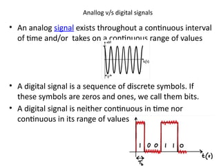
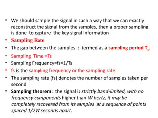
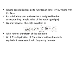
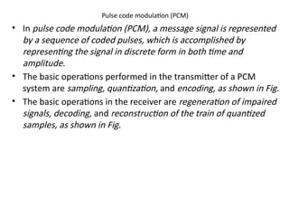
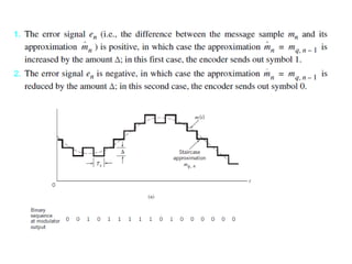
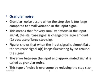
Sampling
• Sampling is the processes of converting continuous -time analog
signal, x (t), into a discrete-time signal x[n] by taking the “samples”
at discrete-time intervals
• An analog signal is converted into a corresponding sequence of
samples that are usually spaced uniformly in time.

• At what rate the samples are selected or what is the interval
between the samples a

• We should sample the signal in such a way that we can exactly
reconstruct the signal from the samples, then a proper sampling
is done to capture the key signal information
• Sampling Rate
• The gap between the samples is termed as a sampling period Ts.
• Sampling Time =Ts
• Sampling Frequency=fs=1/Ts
• fs is the sampling frequency or the sampling rate
• The sampling rate (fs) denotes the number of samples taken per
second
• Sampling theorem: the signal is strictly band-limited, with no
frequency components higher than W hertz, it may be
completely recovered from its samples at a sequence of points
spaced 1/2W seconds apart.

• Nyquist Rate:
• A signal is band-limited with no frequency components higher
than W Hertz. That means, W is the highest frequency.
• For such a signal, for effective reproduction of the original signal,
the sampling rate should be twice the highest frequency
• Which means, fS=2W
• The minimum sampling rate of 2W samples per second is given
by Nyquist and is called as Nyquist rate

Mathematical analysis
• Consider an arbitrary signal g(t) of finite energy,
• Suppose that we sample the signal g(t) instantaneously and at a uniform
rate, once every Ts seconds.
• Consequently, we obtain an infinite sequence of samples spaced Ts
seconds apart and denoted by g{nTs}
• We refer to Ts as the sampling period or sampling interval and to its
reciprocal fs=1/Ts as the sampling rate.

• Consider g(t) that is continuous in both time and amplitude

• Where δ(t-nTs) is dirac delta function at time t=nTs, where n=0,
±1, ±2,...
• Each delta function in the series is weighted by the
corresponding sample value of the input signal g(t)
• We may rewrite the gδ(t) equation as
• Take Fourier transform of the equation
• W .K. T multiplication of 2 functions in time domain is
equivalent to convolution in frequency domain

ALIASING PHENOMENON
• we sample a band-limited signal and choose the sampling
frequency such that fs ≥ 2 f m .
• Notice that in this case the replicas in the sampled signal do not
overlap. This is the principle of the Nyquist rate of sampling.
• Aliasing is caused by sampling at a rate lower than that of the
Nyquist frequency for a given signal
• If , an information bearing signal is not strictly band-limited, some
aliasing is produced by the sampling process
• In practice, however, no information-bearing signal of physical
origin is strictly band-limited,

• Aliasing refers to the phenomenon of a high-frequency component in
the spectrum of the signal seemingly taking on the identity of a lower
frequency in the spectrum of its sampled version, as illustrated
• Aliasing is caused by sampling at a rate lower than that of the Nyquist
frequency for a given signal or if the signal is not strictly bandlimited

• To combat the effects of aliasing in practice, we may use two
corrective measures:
• 1. Prior to sampling, a low-pass( anti-alias filter) is used to
attenuate those high-frequency components of a message signal
that are not essential to the information being conveyed by the
signal.
• 2. The filtered signal is sampled at a rate slightly higher than the
Nyquist rate.
• The use of a sampling rate higher than the Nyquist rate also has
the beneficial effect of easing the design of the synthesis filter
used to recover the original signal from its sampled version.

• The use of a sampling rate
higher than the Nyquist rate
also has the beneficial effect of
easing the design of the
synthesis filter used to recover
the original signal from its
sampled version.

Analog pulse modulation: Pulse amplitude
Modulation
• The simplest and most basic form of analog pulse modulation
techniques.
• In Pulse modulation methods, the carrier is no longer a
continuous signal but consists of a pulse train. Some parameter
of which is varied according to the instantaneous value of the
modulating signal.
• In pulse-amplitude modulation (PAM), the amplitudes of
regularly spaced pulses are varied in proportion to the
corresponding sample values of a continuous message signal

Pulse amplitude Modulation(PAM)

• There are 2 types of PAM: Flat top sampling and
natural sampling
•

Pulse width modulation(PWM)
• The modulating signal may vary the time of occurrence of the
leading edge, the trailing edge or both edges of the pulse

Quantisation
• Introduction: A continuous signal, such as voice, has a
continuous range of amplitudes and therefore its samples
have a continuous( infinite) amplitude range.
• In actual fact it is not necessary to transmit the exact
amplitudes of the samples. We say so because any human
sense (the ear or the eye) as the ultimate receiver can detect
only finite intensity differences.
• The amplitude values of the signal is approximated to the
defined finite values.
• Clearly, if we assign the discrete amplitude levels with
sufficiently close spacing, we can make the approximated
signal indistinguishable from the original continuous signal
• Note also that quantization is non-reversible.

• L is the number of quantisation levels
• ∆ is quantisation step size

Quantizer characteristics
• The peak to peak range of input sample values is sub divided into
finite set of decision levels in the x axis
• The output is assigned a discrete value selected from the finite set of
defined values along y axis

• We have signal with
amplitude ranging from –
8v to +8v
• Let us use L=8
quantisation levels
• Therefore quantisation
step size ∆ = 8-(-8)= 16/8
= 2v
• The 8 zones are -8 to -6, -
6to -4, -4 to -2, -2 to 0, 0
to 2, 2 to 4 , 4 to 6 and 6
to 8

Assignment on Quantisation and encoding
• The signal has amplitude range from -1v to +1v.
i.Quantisize the signal using 8 level quantiser.
ii.. Construct the mid rise and midtread
qunatiser transfer characteristics for the above
quantised signal
• Iii. Construct the encoding table for the
quantised signal.
• Iv. Determine signal to noise ratio of the
quantiser

Important facts about Quantisation
• Quantisation is irreversible process
• Quantisation error is the difference between
the actual sample value and its quantised
value
• Q. Error is reduced by increasing the No. of
quantisation levels(L)
• If L is the number of quantisation levels then
then each level is coded by ‘n’ bits where

Uniform quantiser
• The uniform quantiser is one with a uniform step
size (Δ)

Non Uniform quantiser
• For example, the range of voltages covered by voice signals, from
the peaks of loud talk to the weak talk, is on the order of 1000 to
1.

Pulse code modulation (PCM)
• In pulse code modulation (PCM), a message signal is represented
by a sequence of coded pulses, which is accomplished by
representing the signal in discrete form in both time and
amplitude.
• The basic operations performed in the transmitter of a PCM
system are sampling, quantization, and encoding, as shown in Fig.
• The basic operations in the receiver are regeneration of impaired
signals, decoding, and reconstruction of the train of quantized
samples, as shown in Fig.

• The most important feature of a PCM system lies in the ability
to control the effects of distortion and noise produced by
transmitting a PCM signal over a channel.
• This capability is accomplished by reconstructing the PCM signal
by means of a chain of regenerative repeaters located at
sufficiently close spacing along the transmission route.

• https://www.youtube.com/watch?
v=aH4MzLvHrGI

• three basic functions are performed by a regenerative repeater:
equalization, timing, and decision making.
• The equalizer shapes the received pulses so as to compensate for the effects
of amplitude and phase distortions produced by the transmission
characteristics of the channel.
• The timing circuitry provides a periodic pulse train, derived from the
received pulses; this is done for renewed sampling of the equalized pulses at
the instants of time where the signal-to-noise ratio is a maximum.
• The sample so extracted is compared to a predetermined threshold in the
decision-making device. In each bit interval,
• A decision is then made on whether the received symbol is a 1 or 0 on the
basis of whether the threshold is exceeded or not.
• If the threshold is exceeded, a clean new pulse representing symbol 1 is
transmitted to the next repeater. Otherwise, another clean new pulse
representing symbol 0 is transmitted.
• In this way, the accumulation of distortion and noise in a repeater span is
removed

Differential pulse code modulation DPCM)
• Intro: A voice or video signal is sampled at a rate slightly higher than
the Nyquist rate,
• The resulting sampled signal is found to exhibit a high degree of
correlation between adjacent samples.
• if we know the past behavior of a signal up to a certain point in time,
it is possible to make some inference about its future values; a
process is commonly called prediction.
• If the correlation is exploited, then overall bit rate will decrease and
number of bits required to transmit one sample will also be reduced.
• Principle : we have to predict current sample value based upon
previous samples (or sample) and we have to encode the difference
between actual value of sample and predicted value which is
interpreted as prediction error).
DPCM is form of predictive coding

Working Principle of DPCM
• The DPCM works on the principle of prediction.
• The value of the present sample is predicted from the past
samples.
• The prediction may not be exact but it is very close to the actual
sample value.
• Fig. shows the transmitter of DPCM system.

• The sampled signal is denoted by x(nTs) and predicted signal is
denoted by xˆ(nTs).
• The comparator finds out the difference between the actual sample
value x(nTs) and predicted sample value xˆ(nTs).
• It can be defined as , e(nTs) = x(nTs) – xˆ(nTs)……………………….(1)
• The predicted value is produced by using a prediction filter.
• The quantizer output signal eq(nTs) and previous prediction is
added and given as input to the prediction filter. This signal is
called xq(nTs).
• We can observe that the quantized error signal eq(nTs) is very small
and can be encoded by using small number of bits.
• Thus number of bits per sample are reduced in DPCM.

• The quantizer output can be written as ,
• eq(nTs) = e(nTs) + q(nTs)………………………..(2)
• Here, q(nTs) is the quantization error.
• As shown in fig., the prediction filter input xq(nTs) is obtained by
sum xˆ(nTs) and quantizer output. i.e.,
• xq(nTs) = xˆ(nTs) + eq(nTs)……………………..(3)
• Substituting the value of eq(nTs) from eq.(2) in the above eq. (3) , we get,
• xq(nTs) = xˆ(nTs) + e(nTs) + q(nTs) ………………….(4)
• eq.(1) is written as,
• e(nTs) = x(nTs) – xˆ(nTs)
• ∴ e(nTs) + xˆ(nTs) = x(nTs)
• Therefore, substituing the value of e(nTs) + xˆ(nTs) from the above
equation into eq. (4), we get,
• xq(nTs) = x(nTs) + q(nTs) …………………..(5)

Reception of DPCM Signal
• The decoder first reconstructs the quantized error signal from
incoming binary signal.
• The prediction filter output and quantized error signals are
summed up to give the quantized version of the original signal.
• Thus the signal at the receiver differs from actual signal by
quantization error q(nTs), which is introduced permanently in
the reconstructed signal.

• Advantages of DPCM
• As the difference between x(nTs) and xˆ(nTs) is being encoded
and transmitted by the DPCM technique, a small difference
voltage is to be quantized and encoded.
• This will require less number of quantization levels and hence
less number of bits to represent them.
• Thus signaling rate and bandwidth of a DPCM system will be
less than that of PCM.
•

S. NO Parameters
Pulse Code
Modulation (PCM)
Differential Pulse Code
Modulation (DPCM)
1 Number of bits It uses 4, 8, or 16 bits
per sample
< PCM bits
2 Levels, step size
Fixed step size.
Cannot varied
A fixed number of levels are
used.
3 Bit redundancy Present Can permanently remove
4
Quantization
error and
distortion
Depends on the
number of levels
used
Slope overload distortion and
quantization noise are present
but very less as compared to
PCM
5
The bandwidth of
the transmission
channel
Higher bandwidth
has been required
Lower than PCM bandwidth
6 Feedback No feedback in Tx
and Rx
Feedback exists
7
Complexity of
notation
simple Complex
8
Signal to noise
ratio (SNR)
Good Fair

• Applications of DPCM
• The DPCM technique mainly used in Speech, image and audio
signal compression.
• The DPCM conducted on signals with the correlation between
successive samples leads to good compression ratios.
• In images, there is a correlation between the neighboring pixels,
in video signals, the correlation is between the same pixels in
consecutive frames and inside frames (which is the same as
correlation inside the image).

Delta Modulation
• Delta modulation (DM )is a subclass of differential pulse code
modulation. It can be viewed as a simplified variant of DPCM, in
which 1-bit quantizer is used
• was developed for voice telephony applications.
• In delta modulation (DM), an incoming message signal is
oversampled (i.e., at a rate much higher than the Nyquist rate) to
purposely increase the correlation between adjacent samples of the
signal.
• Unlike PCM, the difference between the input signal and its
approximation is quantized into only two levels—namely,
corresponding to positive and negative differences.
• Thus, if the approximation falls below the input signal at any
sampling epoch, it is increased by +Δ. If, on the other hand, the
approximation lies above the signal, it is diminished by - Δ

• The delta modulator produces a staircase approximation to the
message signal, as illustrated in Figure

Delta modulation Transmitter
• The discrete time equations which describe the delta
modulation

DM receiver
• In the receiver shown in Fig., the staircase approximation is
reconstructed by passing the sequence of positive and negative
pulses, produced at the decoder output and are summed up
with previous sample value to give the quantized version of the
original signal.
• Thus the signal at the receiver differs from actual signal by
quantization error q(nTs), which is introduced permanently in the
reconstructed signal.
• .

08/02/2025 1 72
• The delta modulation are subject two types of
Quantization error :
• Slope overload distortion
• Granular noise
Slope Overload Noise

08/02/2025 1 73
• Slope Overload Noise
• This distortion arises because of large dynamic range of the
input signal.
• We can observe from figure , the rate of rise of input signal
x(t) is so high ( i.e., slope is high) that the staircase signal can
not approximate it, the step size ‘Δ’ becomes too small for
staircase signal u(t) to catch up with the input signal x(t).
• The large error between the staircase approximated signal
and the original input signal x(t) results in noise known
as slope overload distortion.
• To reduce this noise, the step size must be increased when
slope of signal x(t) is high.

08/02/2025 1 74
• Granular noise:
• Granular noise occurs when the step size is too large
compared to small variation in the input signal.
• This means that for very small variations in the input
signal, the staircase signal is changed by large amount
(Δ) because of large step size.
• Figure shows that when the input signal is almost flat ,
the staircase signal u(t) keeps fluctuating by ±Δ around
the signal.
• The error between the input and approximated signal is
called as granular noise.
• This type of noise is overcome by reducing the step size

08/02/2025 1 75
Condition for avoiding slope overload noise
• The staircase approximated signal u(t) should
increase as fast as the input signal i.e.
• Let us consider a sinusoid representing a narrow band
signal x(t)= amcos(2πft ) where ‘f’ represents the
maximum frequency of the signal and ‘am‘ its peak
amplitude. There will be no slope-overload error if

Line Codes
• Intro: we have understood 3 different waveform-coding
schemes: PCM, DPCM, and DM, they differ from each other in
several ways: transmission–bandwidth requirement,
transmitter–receiver structural composition and complexity, and
quantization noise.
• line codes for electrical representation of the encoded binary
streams produced by their individual transmitters, so as to
facilitate transmission of the binary streams across the
communication channel.

https://slideplayer.com/slide/6978771/

• 1. NRZ unipolar (On–off signaling): in which symbol 1 is represented
by transmitting a pulse of constant amplitude for the duration of the
symbol, and symbol 0 is represented by switching off the pulse, as in
Fig. 5.20(a).
• 2. NRZ polar signaling, in which symbols 1 and 0 are represented by
pulses of equal positive and negative amplitudes, as illustrated in Fig.
5.20(b).
• 3. RZ polar signaling, in which symbol 1 is represented by a positive
rectangular pulse of half-symbol width, and symbol 0 is represented
by transmitting no pulse for 0 symbol
• 4. Bipolar return-to-zero (BRZ) signaling, which uses three
amplitude levels as indicated in Fig. 5.20(d). Specifically, positive and
negative pulses of equal amplitude are used alternately for symbol 1,
and no pulse is always used for symbol 0.
• A useful property of BRZ signaling is that the power spectrum of the
transmitted signal has no dc component and relatively insignificant
low-frequency components for the case when symbols 1 and 0 occur
with equal probability.

• Split-phase (Manchester code), which is illustrated in Fig. 5.20(e).
In this method of signaling, symbol 1 is represented by a positive
pulse followed by a negative pulse, with both pulses being of equal
amplitude and half-symbol width.
• For symbol ‘0’, the polarities of these two pulses are reversed.
• The Manchester code suppresses the dc component and has
relatively insignificant low-frequency components,

• RZ bipolar : A polar waveform has no dc component,
provided 0’s and 1’s in the input data occur with
proposition
• Bipolar format has a feature of absence of dc component
• Detection of isolated error due to deletion or creation of
error is possible
• The polarity inversion that occurs during the course of
transmission can be detected
• For this reason it is adopted for T1 digital telephony
• Manchester has built in synchronisation capability
because of their predictable transition during each bit
interval . But this attained at the expense of bandwidth
twice that NRZ unipolar, polar and bipolar formats

Module2.pptxwewewewewewewewewewewewewewewewe

More Related Content

Similar to Module2.pptxwewewewewewewewewewewewewewewewe

Recently uploaded

Module2.pptxwewewewewewewewewewewewewewewewe