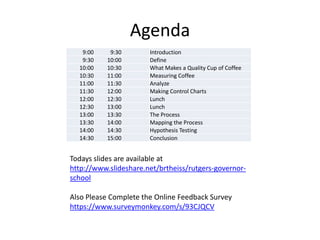
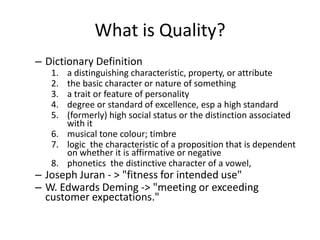
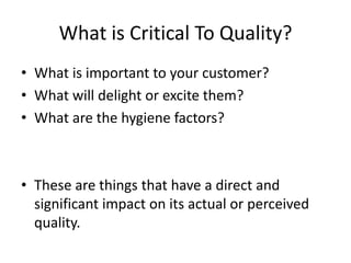
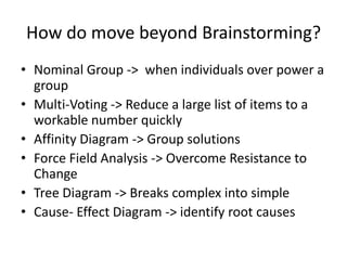
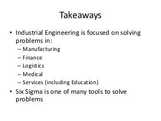
SlideShare a Scribd company logo
Rutgers Governor School

       Introduction
Goals for Today


Show you to see and (perhaps) solve problems differently
•   Academics
                                           About Me
     –   MS Industrial Engineering Rutgers University
     –   BS Electrical & Computer Engineering Rutgers University
     –   BA Physics Rutgers University
•   Professional
     –   Principal Industrial Engineer -Medrtonic
     –   Master Black belt- American Standard Brands
     –   Systems Engineer- Johnson Scale Co
•   Awards
     –   ASQ Top 40 Leader in Quality Under 40
•   Certifications
     –   ASQ Certified Manager of Quality/ Org Excellence Cert # 13788
     –   ASQ Certified Quality Auditor Cert # 41232
     –   ASQ Certified Quality Engineer Cert # 56176
     –   ASQ Certified Reliability Engineer Cert #7203
     –   ASQ Certified Six Sigma Green Belt Cert # 3962
     –   ASQ Certified Six Sigma Black Belt Cert # 9641
     –   ASQ Certified Software Quality Engineer Cert # 4941
•   Publications
     –   Going with the Flow- The importance of collecting data without holding up your processes- Quality Progress March
         2011
     –   "Numbers Are Not Enough: Improved Manufacturing Comes From Using Quality Data the Right Way" (cover story).
         Industrial Engineering Magazine- Journal of the Institute of Industrial Engineers September (2011): 28-33. Print
Agenda
   9:00     9:30       Introduction
   9:30    10:00       Define
  10:00    10:30       What Makes a Quality Cup of Coffee
  10:30    11:00       Measuring Coffee
  11:00    11:30       Analyze
  11:30    12:00       Making Control Charts
  12:00    12:30       Lunch
  12:30    13:00       Lunch
  13:00    13:30       The Process
  13:30    14:00       Mapping the Process
  14:00    14:30       Hypothesis Testing
  14:30    15:00       Conclusion


Todays slides are available at
http://www.slideshare.net/brtheiss/rutgers-governor-
school

Also Please Complete the Online Feedback Survey
https://www.surveymonkey.com/s/93CJQCV
So Lets Get Moving
What is Industrial Engineering?
• is a branch of engineering dealing with the
  optimization of complex processes or systems.
• “Engineers make things. Industrial engineers
  make things better.”
What is a Process?
    • Formal Definition
         – A systematic series of actions directed to some end
    • Practical Definition
         – Any Verb Noun Combination
             • Eat Sandwich
             • Read Book
             • Attend Conference
    • Implications of Practical Definition
         – Same Tools Techniques and Methods of the Lean Six Sigma
           Methodologies can be used for virtually anything
Inputs                                                Outputs
•   People                                            • Products
•   Materials                      Process                • Hardware
•   Methods                        • Sequence of          • Software
•   Mother Nature
                                      Value Added         • Systems
•   Management
•   Measurement
                                      Steps               • People
    System                                            • Services
So How do Make “it” Better
•   Statistics
•   Lean
•   Six Sigma
•   Modeling
Types of Statistics
• Descriptive Statistics
   – Present data in a way that will facilitate understanding
• Inferential Statistics
   – Analyze sample data to infer properties of the
     population from which the sample is drawn

• Statistical Significance Does not Mean actual significance.
   – (See US Supreme Court Matrixx Initiatives, Inc. v.
     Siracusano
Key Descriptive Statistical Terms
              Population Parameters
                                         Size = N
                                         Mean = m
                                         Std. Dev. = s
                                         Proportion = p
                     Sample Statistics


                                          Size = n Mean = x
                                                               ˆ
                                          Std. Dev.= s Prop. = p


                                                               Page 143
Lean Tool Kit
• 5S-
    –   Sort
    –   Straighten
    –   Shine
    –   Standardize
    –   Sustain
•   Value Stream Mapping
•   Kanban
•   Poka-yoke
•   Kaizen <- mean continuous improvement
Six Sigma Tool Kit
• DMAIC
  – Define
  – Measure
  – Analyze
  – Improve
  – Control
• SIPOC Diagrams
• Statistical Process Control
• 5 Whys
Modeling
• A mathematical model is a
  description of a system using
  mathematical concepts and
  language.
                                       Histogram of Time
                                               Weibull
                  25                                                       Shape    2.007
                                                                           Scale   216106
                                                                           N           94

                  20


                  15
      Frequency


                  10


                  5


                  0
                       0   100000   200000      300000   400000   500000
                                             Time
The analogy
 The task is to undo a bolt.


                 Solution 1- Ratchet and Socket


                   Solution 2- Open Ended /Box Wrench


                      Solution 3- Vice Grips


Which is Correct?
The Answer
• It depends.
  – There are certain applications that demand a open
    ended wrench
  – Others require a socket
  – Finally there are situations that require vice grips
• Most cases all three solutions will work
• The same is true for solving Industrial
  Engineering problems
A History Lesson
        Lean
             Mid 1800’s: Interchangeable parts
             1913: Moving assembly line at Ford
             Post-WW2: Toyota Develops a Production System (TPS).
             1996: James Womack documents general application of TPS and for
              any organization and calls it “Lean Thinking”.


    Six Sigma
            Mid-1900s: Shewhart and Deming advocate PDCA methodology
            1980’s: Motorola developed MAIC method for reducing defects in it’s
             products. Won the Baldrige Quality Award in 1988. GE applies Six Sigma
             to non manufacturing
            1990’s-2000’s: Siemens, Allied Signal and others drive 6 Sigma DMAIC
             top-down. Companies in many industries practice Six Sigma, some
             successfully, some not (MDT dabbled in early 1990’s).
16
People to Know
• William Edwards Deming (October 14, 1900 – December 20, 1993) "There
  is no substitute for knowledge.“
    – emphasis on total quality management
• Joseph Moses Juran (December 24, 1904 – February 28, 2008) "It is most
  important that top management be quality-minded. In the absence of
  sincere manifestation of interest at the top, little will happen below."
    - Managing for Quality
• Taiichi Ohno (February 29, 1912 – May 28, 1990) -Toyota
    – Production System (TPS)- Just in Time (JIT)
• Walter Andrew Shewhart ( March 18, 1891 - March 11, 1967) -"Dr.
  Shewhart prepared a little memorandum only about a page in length.
  About a third of that page was given over to a simple diagram which we
  would all recognize today as a schematic control chart.”
    – Control Charts


                                                                 Page 6
What is Six Sigma?
• Six Sigma seeks to improve the quality of process
  outputs by identifying and removing the causes of
  defects (errors) and minimizing variability in
  manufacturing and business processes.
• It uses a set of quality management methods, including
  statistical methods, and creates a special infrastructure
  of people within the organization ("Black Belts",
  "Green Belts", etc.) who are experts in these methods.
• Each Six Sigma project carried out within an
  organization follows a defined sequence of steps
  (DMAIC) and has quantified financial targets (cost
  reduction and/or profit increase).
What is Sigma (s)?

     4 Definitions:

     A letter in the Greek alphabet s

     A statistical measure of variation (standard deviation)

     A measure of a process defect level

     Six Sigma - an improvement methodology (DMAIC)


19
Normal Distribution

• Also known as Gaussian, Laplace–Gaussian or
  standard error curve
• First proposed by de Moivre in 1783
• Independently in 1809 by Gauss

 All Normal Distributions Defined by two things
 1. The Average µ
 2. The Standard Deviation σ


                                                  Page 143
Area Under the Curve
          (c) Probabilities and numbers of standard deviations

   Shaded area = 0.683        Shaded area = 0.954        Shaded area = 0.997


                                                                          
  68% chance of falling         95% chance of falling       99.7% chance of falling
between  and               between   and           between   and          
Effect of Changing Parameters


           (a) Changing                                             (b) Increasing
      shifts the curve along the axis                   increases the spread and flattens the curve

                                                                                               1   =6
                                     1   =   2=   6
                                                                                                    2=   12


140                160         180                200    140            160              180              200

              1   = 160     2 =174                                            1   =   2 =170
What is Process Sigma?
      Before                                                 Customer
                           Mean                              Specification
       3s
                                                                                A 3s process
                                  1s                             Defects        (3 standard
                                       2s                                       deviations fit
                                            3s                                  between target and
                                                                                spec)
                       A 6s process
                          Mean                             Customer
                                                           Specification


               After              1s
                                       2s                         No Defects!
               6s                           3s
                                                 4s
                                                      5s
                                                            6s


23
So what are we going to do?
• We are going to apply DMAIC (Define Measure
  Analyze Improve Control) to the experience of
  going to Starbucks
About Starbucks
• Founded 1971, in Seattle’s Pike Place Market.
  Original name of company was Starbucks
  Coffee, Tea and Spices, later changed to
  Starbucks Coffee Company.
• In United States:
  – 50 states, plus the District of Columbia
  – 7,087 Company-operated stores
  – 4,081 Licensed stores
?
Rutgers Governor School

         Define
What is Quality?
– Dictionary Definition
   1. a distinguishing characteristic, property, or attribute
   2. the basic character or nature of something
   3. a trait or feature of personality
   4. degree or standard of excellence, esp a high standard
   5. (formerly) high social status or the distinction associated
      with it
   6. musical tone colour; timbre
   7. logic the characteristic of a proposition that is dependent
      on whether it is affirmative or negative
   8. phonetics the distinctive character of a vowel,
– Joseph Juran - > "fitness for intended use"
– W. Edwards Deming -> "meeting or exceeding
  customer expectations."
What is Critical To Quality?
• What is important to your customer?
• What will delight or excite them?
• What are the hygiene factors?


• These are things that have a direct and
  significant impact on its actual or perceived
  quality.
How do move beyond Brainstorming?
• Nominal Group -> when individuals over power a
  group
• Multi-Voting -> Reduce a large list of items to a
  workable number quickly
• Affinity Diagram -> Group solutions
• Force Field Analysis -> Overcome Resistance to
  Change
• Tree Diagram -> Breaks complex into simple
• Cause- Effect Diagram -> identify root causes
Nominal Group Technique
• A brainstorming technique that is used when
  some group members are more vocal then
  others and encourages equal participation


                                        Page 114
Nominal Group Procedure
1. Team Leader Selected
2. Individuals Brainstorm for 10-15 minutes
   without talking. Ideas are written down
3. Round Robin each team member reads idea
   and it is recorded by the team leader. There
   is no discussion of ideas.
4. Once all ideas are recorded discussion begins
Multi-Voting
• Multi-voting is a group decision-making
  technique used to reduce a long list of items
  to a manageable number by means of a
  structured series of votes


                                          Page 87
Multi-Voting Procedure
1. Develop a Large Group Brainstormed list
2. Assign a letter to each item
3. Each team member votes for their top 1/3 of
   ideas.
4. Votes are tallied
5. Eliminate all items receiving less than N votes
   (rule of thumb 3)
6. Repeat voting until there are ~4 items left
Multi-Voting Example
Affinity Diagrams
• A tool that gathers large amounts of language
  data (ideas, opinions, issues) and organizes
  them into groupings based on their natural
  relationships


                                         Page 92
Affinity Diagram Procedure
1.   Record Ideas on Post It Notes
2.   Randomize Ideas Together
3.   Sort Ideas into Related Groups
4.   Create Header Card
5.   Record Results
Affinity Diagram Example
1. Randomize Ideas Together     2. Group Ideas


                              4. Put it Together
   3. Create Headers
Force Field Analysis
• Is a method for listing, discussing, and
  assessing the various forces for and against a
  proposed change. It helps to look at the big
  picture by analyzing all of the forces impacting
  on the change and weighing up the pros and
  cons.


                                           Page 109
Force Field Procedure
1. Draw a large letter t
2. At the top of the t, write the issue or problem
3. At the far right of the top of t write the ideal state you wish
   to obtain
4. Fill in the chart
   –   List internal and external factors advancing towards the ideal state
   –   List forces stopping you from obtaining the ideal state
Force Field Example
Tree Diagram
• Tree diagrams help link a task’s overall goals
  and sub-goals, and helps make complex tasks
  more visually manageable. Accomplished
  through successive steps digging into deeper
  detail.


                                           Page 124
Tree Diagram Procedure
1. Identify the Goal
2. Generate Tree Headings (Sub Goals)
  – ~5 slightly more specific topics that are related to
    the general goal
  – Place them horizontally on post it notes
    horizontally under goal
3. Generate Branches of sub goals as needed
4. Record the results
Tree Diagram Example
Cause and Effect Diagram
     (Fishbone or Ishikawa Diagram)
• Is a tool that helps identify, sort, and display
  possible causes of a specific problem or
  quality characteristic. It graphically illustrates
  the relationship between a given outcome and
  all the factors that influence the outcome.


                                             Page 97
Cause and Effect Procedure
1. Identify and Define the Effect
2. Draw the Fishbone Diagram
  – Place Effect as the Head of the fish
3. Identify categories for the main causes of the
   effect or use the standard ones
   (Man, Machine, Methods, Materials, Measur
   ements, Mother Nature)
4. Add causes to the categories
5. Add increasing detail to describe the cause
Cause and Effect Example
Generic Format      1. Identify Categories


2. Add Causes        3. Add Details
Now Apply It!
• Divide yourself into 6 Groups
  –   Group 1- Nominal Group
  –   Group 2- Multi-Voting
  –   Group 3- Affinity Diagrams
  –   Group 4- Force Field Analysis
  –   Group 5- Tree Diagram
  –   Group 6- Cause and Effect Diagram (What Causes a
      Bad Cup of Coffee)
• Solve the problem “What Makes a Quality Coffee
  Experience?”
Rutgers Governor School

        Measure
Types of Data
                                              Variable / Continuous Data
• Attribute    / Discrete Data                      Individual unit can be measured on
– Individual unit categorized into a                 a continuum or scale Examples:
  classification. Examples:                           • Length
    • Counts or frequencies of occurrence             • Volume
      (# of errors, # of units)                       • Time
                                                      • Size
    • Categories (good/bad, pass/fail,
                                                      • Width
      low/medium/high)
                                                      • Pressure
    • Characteristics (locations, shift #,            • Temperature
      male/female)                                    • Thickness
    • Groups (complaint codes, error                Can have almost any numeric value
      codes, problem type)
                                                    Can be meaningfully subdivided
– Finite number of values is possible                into finer increments
– Cannot be subdivided meaningfully


                                                                               Page 110
Data Type – Why is this
                                important?
                                      Data type is a key driver of your Project Strategy
                                                                                                                                                               
                   Attribute / Discrete Data                                                                                       Variable / Continuous Data
                                       Requires larger sample size                                                                •      More analysis tools available
                                       Usually readily available                                                                  •      Smaller sample size needed
                    To see variation you stratify                                                                                 •      Higher confidence in results
                                                                                                                                   •     To see variation, you can also
                                Pareto Chart
                                      100%
                                      80%
                                                                                                                                        look at the distribution
                                      60%
                                                                                                                                   Dotplot                                                                                                                 Histogram
                                      40%
                                      20%
                                        0%
                                                       FM                     OD           ID     Burr
                                                                                                         Control Chart
       Control Chart
                                      P Chart of Resolved
                                                                                                         for Individuals
                                                                                                          4%
             0.4                                                                                              % Defective      1
                                                                                                                                       Descriptive Statistics
                                                            1
                                                                                                                                                                          Summary for Mystery
                                                                                     UCL=0.3539
                                                                                                         3%
             0.3
                                                                                                                                                                                                                    A nderson-D arling N ormality Test
                                                                                                                                                                                                                         A -S quared
                                                                                                                                                                                                                         P -V alue <
                                                                                                                                                                                                                                           27.11
                                                                                                                                                                                                                                           0.005
                                                                                                                                                                                                                                                           Individuals Chart
Proportion


                                                                                     _                   2%
                                                                                                                                                                                                                         M ean
                                                                                                                                                                                                                         S tDev
                                                                                                                                                                                                                         V ariance
                                                                                                                                                                                                                                           100.00
                                                                                                                                                                                                                                            32.38
                                                                                                                                                                                                                                          1048.78
                                                                                                                                                                                                                                                           4%
             0.2                                                                     P=0.1972                                                                                                                            S kew ness
                                                                                                                                                                                                                         Kurtosis
                                                                                                                                                                                                                         N
                                                                                                                                                                                                                                          0.00716
                                                                                                                                                                                                                                         -1.63184
                                                                                                                                                                                                                                              500
                                                                                                                                                                                                                                                                % Defective      1


             0.1                                                                                         1%                                                                                                              M inimum
                                                                                                                                                                                                                         1st Q uartile
                                                                                                                                                                                                                         M edian
                                                                                                                                                                                                                                           41.77
                                                                                                                                                                                                                                           68.69
                                                                                                                                                                                                                                          104.20
                                                                                                                                                                                                                                                           3%
                                                                                                                                                                                                                         3rd Q uartile    130.81
                                                                                                                                                 40   60         80      100      120            140   160
                                                                                                                                                                                                                         M aximum         162.82
                                                                                     LCL=0.0404                                                                                                                    95% C onfidence Interv al for M ean

             0.0                                                                                         0%                                                                                                              97.15            102.85
                                                                                                                                                                                                                   95% C onfidence Interv al for M edian
                                                                                                                                                                                                                                                           2%
                                                                                                                                                                                                                         82.78            117.66
                   1/29   3/5   4/9   5/14    6/18   7/23       8/27   10/1   11/5
                                                                                                                                                                                                                   95% C onfidence Interv al for S tDev
                                             Week                                                                                                               95% Confidence Intervals


Tests performed with unequal sample sizes
                                                                                                                        Days             Mean
                                                                                                                                                                                                                         30.49             34.53

                                                                                                                                                                                                                                                           1%
                                                                                                                                        Median

                                                                                                                                                 80        90             100              110               120


             52                                                                                                                                                                                                                                            0%
                                                                                                                                                                                                                                                                          Days
So how do we translate our CTQs Into
           Measurements?

• Quality Functional
  Deployment (House of
  Quality)
• “Whats into Hows”


                    Y   into Y into x


From the Customer        Means Something   You Can Measure it`
                         Internally
So What are We Going To Measure?
– Taste (what is taste?)
   • pH
   • Total Dissolved Solids
   • Temperature
– Consistency
   • Weight of the beverage
   • Taste
Go Measure!
• Create the Following Control Charts
  – Group 1: Starbucks Regular
  – Group 2: Starbucks Decaffeinated
  – Group 3: Dunkin Donuts Regular
  – Group 4: Dunkin Donuts Decaffeinated
So How Do We Display the Data?
•   Dot Plot
•   Run Chart
•   Box Whisker Plot
•   CUSUM
•   EWMA
•   Scatter Diagrams
•   Pareto Charts
Dot Plot


• Is a statistical chart consisting of data points
  plotted on a simple scale, typically using filled in
  circles representing the frequency of observation
                                               Page 164
Run Chart


• Is a graph that displays observed data in a time
  sequence. Often, the data displayed represent
  some aspect of the output or performance of a
  manufacturing or other business process.
                                             Page 166
Box Plot
        (Box and Whisker Diagram)
• Is a graphic depiction of groups of
  numerical data through their five-
  number summaries: the smallest
  observation (sample minimum), lower
  quartile (Q1), median (Q2), upper
  quartile (Q3), and largest observation
  (sample maximum). A boxplot may also
  indicate which observations, if any,
  might be considered outliers.


                                           Page 164
CUSUM
         (Cumulative Sum Chart)


• Is a sequential analysis technique used for
  monitoring changes
EWMA
 (Exponential Weight Moving Average)


• Is a type of control chart used to monitor either
  variables or attributes-type data using the monitored
  business or industrial process's entire history of output
Scatter Diagrams


• Is used to display a relationship or association
  between two variables


                                            Page 167
Pareto Chart


• Named after Vilfredo Pareto, is a type of chart that contains both
  bars and a line graph, where individual values are represented in
  descending order by bars, and the cumulative total is represented
  by the line.

                                                             Page 136
Control Chart
• Time plot of data with Center Line (mean average) & Control Limits
     – Control limits are based on actual process variation (Not specs!)
              • UCL = X-bar (i.e., data mean) + 3s; LCL = X-bar - 3s
     40

     35                                                        Upper Control Limit
                                                                      (UCL)
     30

     25
                                                                         Center Line
                                                                         (X-bar)
     20
                                                               Lower Control Limit
     15
                                                                         (LCL)
     10


          0           5          10         15          20         25

 Voice Of the Process (X-bar, UCL, LCL are based on actual data!):
      Control Limits and Center Line reflect process variation and stability
      A process is predictable (stable) when data points vary randomly within control
       limits. Referred to as a process “in control.”
64                                                                               Page 110
Before Using Control Charts Check for Normality
                                                       Histogram of Normal                                                                         Probability Plot of Normal
                         100                                                                                                                                 Normal
                                                                                                                  99.9
                                                                                                                                                                                                 Mean        168.0
                                                                                                                                                                                                 StDev       24.00
                            80                                                                                      99
                                                                                                                                                                                                 N             500
                                                                                                                                                                                                 AD          0.418
                                                                                                                    95                                                                           P-Value     0.328
                                                                                                                    90
                            60
            Frequency


                                                                                                                    80
                                                                                                                    70


                                                                                                      Percent
                                                                                                                    60
                            40                                                                                      50
                                                                                                                    40
                                                                                                                    30
                                                                                                                    20
                            20                                                                                      10
                                                                                                                     5

                                                                                                                     1
                                0
                                          90          120          150        180      210    240
                                                                     Normal                                        0.1
                                                                                                                             50          100               150           200             250
                                                                                                                                                          Normal


                                                      Histogram of Positive
                 200                                                                                                                           Probability Plot of Positive
                                                                                                                                                             Normal
                                                                                                                  99.9
                                                                                                                                                                                               Mean          168.0
                                                                                                                                                                                               StDev         24.00
                 150                                                                                               99
                                                                                                                                                                                               N               500
                                                                                                                                                                                               AD           46.489
                                                                                                                   95                                                                          P-Value      <0.005
Frequency


                                                                                                                   90

                 100                                                                                               80
                                                                                                                   70


                                                                                                     Percent
                                                                                                                   60
                                                                                                                   50
                                                                                                                   40
                                                                                                                   30
                    50                                                                                             20
                                                                                                                   10
                                                                                                                    5


                        0                                                                                           1
                                    150         180          210           240         270     300
                                                                    Positive                                       0.1
                                                                                                                                  100        150          200          250         300
                                                                                                                                                         Positive


                                                      Histogram of Negative                                                                    Probability Plot of Negative
                                                                                                                                                             Normal
                                                                                                                   99.9
                        250                                                                                                                                                                    Mean         168.0
                                                                                                                                                                                               StDev        24.00
                                                                                                                     99
                                                                                                                                                                                               N              500
                        200                                                                                                                                                                    AD          44.491
                                                                                                                     95                                                                        P-Value     <0.005
                                                                                                                     90
     Frequency


                                                                                                                     80
                        150                                                                                          70
                                                                                                        Percent


                                                                                                                     60
                                                                                                                     50
                                                                                                                     40
                        100                                                                                          30
                                                                                                                     20
                                                                                                                     10
                                                                                                                         5
                        50
                                                                                                                         1

                            0                                                                                       0.1
                                     0         30       60          90           120    150    180                                0     50            100        150         200         250
                                                                   Negative
                                                                                                                                                        Negative
                                                                                                                                                                                                                     Page 173
Control Chart Decision Tree
                                    Variable (continuous)                               Attribute (discrete)
                                                                What Type Of Data?

                                                                                                            Counting
                          Data Collected In
                                                                                                            Specific Defects or
                          Groups or Individuals?
                                                                                                            Defective Items?
     GROUPS                                        INDIVIDUAL
     (Averages)                                    VALUES                         Specific                                                 Defective
     (n>1)                                         (n=1)                          Types Of                                                 Items
                                                                                  “Defects”

X-Bar R (Means w/Range)             Individuals (I Chart)
X-Bar S (Means w/St Dev)            With Moving Range (I-MR)                   You can count only                                 You can count how
                                                                               defects                                            many are bad and
                                                                                                                                  how many are good
NOTE: X-Bar S is appropriate
                                                                                 Poisson Distribution                             Binomial Distribution
for subgroup sizes of > 10


                                                                                     Area of
                                                                                                                                         Constant
                                                                                     Opportunity Constant
                                                                                                                                         Sample Size?
                                                                                     In Each Sample
                                                                                     Size?


                                                                            NO                    YES                              NO                   YES
                                                                        u Chart               c Chart or                      p Chart            np Chart or
                                                                                              u Chart                                            p Chart

                                                                                                                                               Page 110
X-Bar R


          Page 313
X-Bar S


          Page 315
P Chart


Used to monitor the proportion of nonconforming units in a sample, where the
sample proportion nonconforming is defined as the ratio of the number of
nonconforming (defective) units to the sample size, n


                                                                          Page 319
Np Chart
                                          NP Chart of Wrong Answers
               40
                                                                                  1

                                               1
               30                     1
                                                                 1
                             1   1
Sample Count


                                                                                            UCL=24.25

               20
                                                                                            __
                                                                                            NP=15.44

               10
                                                                                            LCL=6.63
                        11
                                                                              1
               0                                                     1
                    1    6       11       16       21     26     31      36       41   46
                                                        Sample


     Used to monitor the number of nonconforming units in a sample. It is an
     adaptation of the p-chart and used in situations where personnel find it easier
     to interpret process performance in terms of concrete numbers of units rather
     than the somewhat more abstract proportion.


                                                                                                        Page 321
I-MR


       Page 317
Words Have Meaning
• Defect
  – any nonconformance of the unit of product with
    the specified customer requirements
• Defective
  – is a unit of product which contains one or more
    defects that effects the operability of the product
    as determined by the customer
C Chart


Used to monitor "count"-type data, typically total number of nonconformities
(defects) per unit. It is also occasionally used to monitor the total number of
events occurring in a given unit of time.


                                                                              Page 325
U Chart


used to monitor "count"-type data where the sample size is greater than one,
typically the average number of nonconformities per unit


                                                                           Page 323
Interpretation
Page 369
Now Apply it
• Create the Following Control Charts
  – Group 1: I-MR Chart for pH
  – Group 2: I-MR Chart for Temperature
  – Group 3: I-MR Chart for TDS
  – Group 4: I-MR Chart for Weight
Regular Starbucks
                                                  I-MR Chart of Temp                                                                                                     I-MR Chart of TDS
                     130                                                                                                     108.0                                                                             U C L=107.751
                                                                                       U C L=128.95
                                                                                                                             106.5
Individual Value


                                                                                                      Individual Value
                     125
                                                                                       _                                     105.0                                                                             _
                                                                                       X=122.69                                                                                                                X=104.5

                     120                                                                                                     103.5

                                                                                                                             102.0
                                                                                       LC L=116.43
                                                                                                                                                                                                               LC L=101.249
                     115
                                  1   2   3   4      5           6   7    8   9   10                                                                 1       2   3   4        5         6    7   8   9   10
                                                     O bser vation                                                                                                           O bser vation


                              8                                                                                                              4                                                                 U C L=3.993
                                                                                       U C L=7.696

                              6                                                                                                              3


                                                                                                                             M oving Range
              M oving Range


                              4                                                                                                              2
                                                                                       __                                                                                                                      __
                                                                                       M R=2.356                                                                                                               M R=1.222
                              2                                                                                                              1


                              0                                                        LC L=0                                                0                                                                 LC L=0
                                  1   2   3   4      5           6   7    8   9   10                                                                 1       2   3   4        5         6    7   8   9   10
                                                     O bser vation                                                                                                           O bser vation


                                                   I-MR Chart of PH                                                                                                      I-MR Chart of Mass
                     5.0                                                                                                                                                                                        U C L=176.60
                                                                                       U C L=4.815                           175


                                                                                                      Individual Value
Individual Value


                     4.5                                                                                                     170
                                                                                                                                                                                                                _
                                                                                       _                                     165                                                                                X=164.78
                                                                                       X=4.135
                     4.0
                                                                                                                             160

                                                                                                                             155
                     3.5                                                               LC L=3.455                                                                                                               LC L=152.96
                                  1   2   3   4      5           6   7    8   9   10                                                             1       2       3   4      5           6    7   8   9    10
                                                     O bser vation                                                                                                          O bser vation


                                                                                       U C L=0.8350                             16
                     0.8                                                                                                                                                                                        U C L=14.52

                                                                                                                                12
M oving Range


                                                                                                             M oving Range


                     0.6


                     0.4                                                                                                              8
                                                                                       __                                                                                                                       __
                                                                                       M R=0.2556                                                                                                               M R=4.44
                     0.2                                                                                                              4


                     0.0                                                               LC L=0                                         0                                                                         LC L=0
                                  1   2   3   4      5           6   7    8   9   10                                                             1       2       3   4      5           6    7   8   9    10
                                                     O bser vation                                                                                                          O bser vation
Decaf Starbucks
                                              I-MR Chart of Temp                                                                                       I-MR Chart of PH
                                                                              1                                                   5
                                                                      1                                                                                                                     U C L=4.929
                                                                                   U C L=122.36
                    122
Individual V alue


                                                                                                              Individual V alue
                                                                                                                                  4
                    120
                                                                                   _                                                                                                        _
                    118                                                            X=118.13                                       3                                                         X=2.946

                    116                                                                                                           2

                    114                                                            LC L=113.90                                    1                                                         LC L=0.963
                                  1
                              1   2   3   4      5           6   7    8   9   10                                                       1   2   3   4      5           6   7   8   9   10
                                                 O bser vation                                                                                            O bser vation


                                                                                   U C L=5.191                            2.4                                                               U C L=2.436
                    4.8
   M oving Range


                                                                                                  M oving Range
                                                                                                                          1.8
                    3.6

                    2.4                                                                                                   1.2
                                                                                   __                                                                                                       __
                                                                                   M R=1.589                                                                                                M R=0.746
                    1.2                                                                                                   0.6


                    0.0                                                            LC L=0                                 0.0                                                               LC L=0
                              1   2   3   4      5           6   7    8   9   10                                                       1   2   3   4      5           6   7   8   9   10
                                                 O bser vation                                                                                            O bser vation


                                              I-MR Chart of Mass                                                                                       I-MR Chart of TDS
                                                                                                                                       1
                                                                                    U C L=84.38                           200
                    80
Individual V alue


                                                                                                  Individual V alue
                                                                                                                          190

                                                                                    _                                     180                                                              U C L=180.62
                    70                                                              X=69.81
                                                                                                                                                                                           _
                                                                                                                          170                                                              X=168.5
                    60
                                                                                                                          160
                                                                                    LC L=55.24                                                                                             LC L=156.38
                          1       2   3   4      5           6   7    8   9   10                                                       1   2   3   4      5           6   7   8   9   10
                                                 O bser vation                                                                                            O bser vation

                                                                                                                                           1
                    20
                                                                                    U C L=17.90
                                                                                                                                  20
                    15
                                                                                                         M oving Range
M oving Range


                                                                                                                                  15                                                       U C L=14.88
                    10
                                                                                                                                  10
                                                                                    __
                     5                                                              M R=5.48                                                                                               __
                                                                                                                                   5                                                       M R=4.56

                     0                                                              LC L=0                                         0                                                       LC L=0
                          1       2   3   4      5           6   7    8   9   10                                                       1   2   3   4      5           6   7   8   9   10
                                                 O bser vation                                                                                            O bser vation
Regular Dunkin Donuts
                                                I-MR Chart of Temp                                                                            I-MR Chart of TDS
                        144                                                                                                 180   1
                                                                                      U C L=143.28
                                                                                                                                                                               U C L=169.16
Individual V alue


                                                                                                     Individual V alue
                        141                                                                                                 165

                                                                                      _                                     150                                                _
                        138                                                           X=137.77                                                                                 X=147.13

                                                                                                                            135
                        135
                                                                                                                                                                               LC L=125.09
                                                                                      LC L=132.27                           120                                        1
                        132                                                                                                                                                1
                                    1   2   3      4             5    6   7   8                                                   1   2   3      4             5   6   7   8
                                                    O bser vation                                                                                 O bser vation


                                                                                      U C L=6.768                            30
                                                                                                                                                                               U C L=27.07
                           6.0
   M oving Range


                                                                                                            M oving Range
                           4.5                                                                                               20


                           3.0
                                                                                      __                                                                                       __
                                                                                      M R=2.071                              10
                                                                                                                                                                               M R=8.29
                           1.5

                           0.0                                                        LC L=0                                  0                                                LC L=0
                                    1   2   3      4             5    6   7   8                                                   1   2   3      4             5   6   7   8
                                                    O bser vation                                                                                 O bser vation


                                                 I-MR Chart of PH                                                                             I-MR Chart of Mass
                                                                                       U C L=3.273                          140
                                3                                                                                                                                              U C L=135.25
            Individual V alue


                                                                                                     Individual V alue
                                                                                                                            130

                                2                                                      _
                                                                                       X=1.81                                                                                  _
                                                                                                                            120
                                                                                                                                                                               X=118.22

                                1
                                                                                                                            110

                                                                                       LC L=0.347
                                                                                                                            100                                                LC L=101.20
                                0
                                    1   2   3      4              5   6   7       8                                               1   2   3      4             5   6   7   8
                                                    O bser vation                                                                                 O bser vation


                        2.0                                                                                                                                                    U C L=20.91
                                                                                                                             20
                                                                                       U C L=1.797
                        1.5
                                                                                                            M oving Range
M oving Range


                                                                                                                             15

                        1.0                                                                                                  10
                                                                                       __                                                                                      __
                                                                                       M R=0.55                                                                                M R=6.4
                        0.5                                                                                                   5


                        0.0                                                            LC L=0                                 0                                                LC L=0
                                    1   2   3      4              5   6   7       8                                               1   2   3      4             5   6   7   8
                                                    O bser vation                                                                                 O bser vation
Decaf Dunkin Donuts
                                     I-MR Chart of Temp                                                                                  I-MR Chart of TDS

                   122                                                    U C L=122.357                        140                                                             U C L=140.33
Individual Value


                                                                                          Individual Value
                   120
                                                                          _                                    135                                                             _
                   118                                                    X=117.988                                                                                            X=134.25


                   116
                                                                                                               130
                   114                                                                                                                                                         LC L=128.17
                                                                          LC L=113.618
                                                                                                                                                                       1
                         1   2   3      4             5   6   7   8                                                          1   2   3      4             5    6   7   8
                                         O bser vation                                                                                       O bser vation


                   6.0                                                                                                   8
                                                                                                                                                                               U C L=7.468
                                                                          U C L=5.368
                   4.5                                                                                                   6
  M oving Range


                                                                                                        M oving Range
                   3.0                                                                                                   4

                                                                          __                                                                                                   __
                   1.5                                                    M R=1.643                                      2                                                     M R=2.286


                   0.0                                                    LC L=0                                         0                                                     LC L=0
                         1   2   3      4             5   6   7   8                                                          1   2   3      4             5    6   7   8
                                         O bser vation                                                                                       O bser vation


                                      I-MR Chart of PH                                                                                   I-MR Chart of Mass
                                                                           U C L=4.3083                        300
                                                                                                                                                                                U C L=285.9
Individual Value


                   4.2

                                                                                          Individual Value
                                                                                                               250

                                                                           _                                                                                                    _
                                                                           X=4.0575                            200                                                              X=201.6
                   4.0
                                                                                                               150

                                                                                                                                                                                LC L=117.2
                   3.8                                                     LC L=3.8067
                                                                                                               100
                         1   2   3      4             5   6   7       8                                                      1   2   3      4              5   6   7       8
                                         O bser vation                                                                                       O bser vation


                   0.3                                                     U C L=0.3081                        100                                                              U C L=103.6
M oving Range


                                                                                          M oving Range


                                                                                                                        75
                   0.2

                                                                                                                        50
                                                                           __                                                                                                   __
                   0.1                                                     M R=0.0943                                                                                           M R=31.7
                                                                                                                        25


                   0.0                                                     LC L=0                                        0                                                      LC L=0
                         1   2   3      4             5   6   7       8                                                      1   2   3      4              5   6   7       8
                                         O bser vation                                                                                       O bser vation
Rutgers Governor School

    Mapping The Process
What is a Process?
• A Process


• Remember “Verb-Noun Combination”
Graphically Presenting a Process
• Six Sigma
  – SIPOC
  – Process Mapping
• Lean
  – Value Stream Map


         Let the Picture do the talking
Suppliers Inputs Process Outputs
           Customers (SIPOC)
• Is a high-level picture of a process that depicts
  how the given process is servicing the
  customer.


                                                Page 51
SIPOC Procedure
1.   Agree to the name of the process. Use a Verb + Noun format (e.g.
     Recruit Staff).
2.   Define the Outputs of the process. These are the tangible things
     that the process produces (e.g. a report, or letter).
3.   Define the Customers of the process. These are the people who
     receive the Outputs. Every Output should have a Customer.
4.   Define the Inputs to the process. These are the things that trigger
     the process. They will often be tangible (e.g. a customer request)
5.   Define the Suppliers to the process. These are the people who
     supply the inputs. Every input should have a Supplier. In some
     “end-to-end” processes, the supplier and the customer may be
     the same person.
6.   Define the sub-processes that make up the process. These are the
     activities that are carried out to convert the inputs into outputs.
     They will form the basis of a process map.
SIPOC Symbols
• Suppliers: The individuals, departments, or organizations that
  provide the materials, information, or resources that are worked on
  in the process being analyzed

• Inputs: The information or materials provided by the suppliers.
  Inputs are transformed, consumed, or otherwise used by the
  process (materials, forms, information, etc.)

• Process: The macro steps (typically 4-6) or tasks that transform the
  inputs into outputs: the final products or services

• Outputs: The products or services that result from the process.
SIPOC Example
Process Maps
• Are a graphical outline or schematic drawing
  of the process to be measured and improve.


                                             Page 128
Process Map Procedure
1. Identify the process to be studied, identify
   boundaries and interfaces
2. Determine Various Steps in the process
3. Build the Sequence of Steps
4. Draw the formal chart with process map
5. Verify Completeness
Process Map Symbols
Process Map Example
Value Stream Mapping (VSM)
• Special type of flow chart that uses symbols
  known as "the language of Lean" to depict
  and improve the flow of inventory and
  information
• Purpose
  – Provide optimum value to the customer through
    a complete value creation process with minimum
    waste


                                               Page 24
VSM Procedure
Before doing any steps, determine who owns the process!
1. Identify Process Customers (Y Process Output
   Measures)
2. Identify Process Suppliers
3. Map the Material (Process) Flow
     •   Process General Steps
     •   Queue or Staging Areas
4.   Identify Process Information Systems
5.   Map the Information Flow
6.   Identify Common Data
7.   Gather the Data
Common VSM Symbols

                  Electronic Communication                     Dotted Line represents
                  Information Flow                             manual process connection


                                                               Box with Jagged top
                                                               represents interaction with
                  Manual Information Flow       Customer       customer or supplier.


                   Red Box and Rectangle                       Block represents a process
     Production
       Control     represents information    MSD Cust. Srvc.   step that is performed.
                   system used.
       MRP


95
Determine Process Cycle Times &
        Identify Value Added Steps

VA


                                                                              NVA


     Value Added Steps are anything that the customer is willing to pay for
VSM Example
Links to the Videos
• Latte : http://youtu.be/HyAAxMEdB24

• Frap : http://youtu.be/3qk28eEbfc4

• Drip : http://youtu.be/IGuwC1WcjKY

• Clover : http://youtu.be/YtXClUKhLmw
Now Apply It!
• Create a SIPOC, Process Map or Value Stream
  Map for the “make drink” process
  – Latte
  – Frappuccino
  – Drip Coffee
  – Clover
Rutgers Governor School

        Analyze
What is an Hypothesis Test?
         Hypothesis Test determines which is more likely to be true:
              Null hypothesis (Ho) or Alternative hypothesis (Ha)
         Ho always starts with “There is no difference between….”


p-Value:                Probability Ho is true given the evidence
If p is low:                      Reject Ho and accept Ha


Example:
Null hypothesis (Ho):             Defendant is guilty (not a Key X)
Alternative Hypothesis (Ha):                 Defendant is not guilty     (A Key X)
p-Value:                                     Probability defendant is not guilty given the evidence
If p is small (reasonable doubt): Reject Ho and conclude defendant is not guilty (Key X!)


    101
Steps in Test of Hypothesis
1.   Formulate the Null and Alternate Hypothesis
2.   Determine the appropriate test
3.   Establish the level of significance:α
4.   Determine whether to use a one tail or two tail test
5.   Determine the degree of freedom
6.   Calculate the test statistic
7.   Compare computed test statistic against a tabled/critical
     value

• Remember: tests    DON’T PROVE anything.
     – They gather sufficient evidence against the null hypothesis Ho
       or fail to gather sufficient evidence against Ho.


                                                                        102
Formulate the null and alternative hypotheses.

 a. NULL HYPOTHESIS (H0): H0 specifies a value for the population parameter
    against which the sample statistic is tested. H0 always includes an
    equality.


b. ALTERNATIVE HYPOTHESIS (Ha): Ha specifies a competing value for the
   population parameter.
   Ha is formulated to reflect the proposition the researcher wants to verify.
   Ha always includes a non-equality that is mutually exclusive of H0.
   Ha is set up for either a 1-tailed test or a 2-tailed test.
Determine The Appropriate Test
• Z
   – is any statistical test for which the distribution of the test statistic
     under the null hypothesis can be approximated by a normal
     distribution.
• T
   – is any statistical hypothesis test in which the test statistic follows a
     Student's t distribution if the null hypothesis is supported
• Paired T
   – is a test that the differences between the two observations is 0
• ANOVA
   – Is a test to determine the differences between two or more
     treatments
• Chi Squared
   – Is a test to determine the goodness of fit of data to a distribution
• Lots of Other Tests
Choose α, our significance level

It really depends on what we are testing

– α = 0.05

– α = 0.01

– Type I error


                                           105
Find the critical value of the test statistic

• Standard normal table

• Student’s t distribution table

• Two-sided vs. one-sided

• F Distribution Table

• Chi Square Distribution Table


                                             106
Two-sided tests  Zα/2


                         107
One-sided tests  Zα


                       108
F Table
Compare the observed test statistic with
          the critical value


                               -Zcrit        Zcrit
  | Ztest | > | Zcrit | HA
  | Ztest |  | Zcrit | H0            H0
                                   HA                HA


                                                          110
Compare the observed test statistic with
          the critical value


                               -1.96        1.96
                                       H0
   | Ztest | > | 1.96 | HA
   | Ztest |  | 1.96 | H0     HA          HA


                                                   111
Compare the observed test statistic with
      the critical value (1 Tail)


    Ztest > 1.645 HA        1.645
    Ztest  1.645 H0   H0

                               HA


                                       112
p-value
• p-value is the probability of getting a value of the test
  statistic as extreme as or more extreme than that observed
  by chance alone, if the null hypothesis H0, is true.

• It is the probability of wrongly rejecting the null
  hypothesis if it is in fact true

• It is equal to the significance level of the test for which
  we would only just reject the null hypothesis


                                                            113
The Chi Square Test
• A statistical method used to determine goodness
  of fit
  – Goodness of fit refers to how close the observed data
    are to those predicted from a hypothesis


• Note:
  – The chi square test does not prove that a hypothesis is
    correct
     • It evaluates to what extent the data and the hypothesis have
       a good fit
Purpose of ANOVA
• Use one-way Analysis of Variance to test when the mean of
  a variable (Dependent variable) differs among two or more
  groups
    – For example, compare whether systolic blood pressure differs
      between a control group and two treatment groups
•   One-way ANOVA compares two or more groups defined
    by a single factor.
    – For example, you might compare control, with drug treatment
      with drug treatment plus antagonist. Or might compare control
      with five different treatments.
•   Some experiments involve more than one factor. These
    data need to be analyzed by two-way ANOVA or Factorial
    ANOVA.
    – For example, you might compare the effects of three different
      drugs administered at two times. There are two factors in that
      experiment: Drug treatment and time.
What Does ANOVA Do?
• ANOVA involves the partitioning of variance of the
  dependent variable into different components:
   – A. Between Group Variability
   – B. Within Group Variability
• More Specifically, The Analysis of Variance is a method
  for partitioning the Total Sum of Squares into two
  Additive and independent parts.


                                                            116
Test Statistic in ANOVA
• F = Between group variability / Within group variability
   – The source of Within group variability is the individual
     differences.
   – The source of Between group variability is effect of independent
     or grouping variables.
   – Within group variability is sampling error across the cases
   – Between group variability is effect of independent groups or
     variables


                                                                   117
ANOVA is Appropriate if:
• Independent random samples have been taken from each population
• Dependent variable population are normally distributed (ANOVA is
  robust with regards to this assumption)
• Population variances are equal (ANOVA is robust with regards to this
  assumption)
• Subjects in each group have been independently sampled


                                                                     118
ANOVA Hypothesis

• Ho: m1 = m2 = m3 = m4
    Where
      •   m1 = population mean for group 1
      •   m2 = population mean for group 2
      •   m3 = population mean for group 3
      •   m4 = population mean for group 4
• H1 = not Ho


                                             119
ANOVA Compare the Computed Test
   Statistic Against a Tabled Value
• α = .05
• If Ftest > FCritcal Reject H0
• If Ftest <= FCritcal Can not Reject H0

              Fα is found in table on 374
              or using Excel FINV function
Rutgers Governor School - Six Sigma

More Related Content

Similar to Rutgers Governor School - Six Sigma

SIX SIGMA
SIX SIGMA SIX SIGMA
SIX SIGMA
Kumar Kunal
 
Six sigma
Six sigmaSix sigma
Six sigma
Kumar Kunal
 
3 16-01 six-sigma
3 16-01 six-sigma3 16-01 six-sigma
3 16-01 six-sigma
Ayanle Hussein
 
Six sigma
Six sigma Six sigma
Six sigma
Suraj Satpathy
 
Yellow belt training program
Yellow belt training programYellow belt training program
Yellow belt training program
Narendra Narendra
 
Apply six sigma with ease @ 3rd Annual Lean Conference, 2015.
Apply six sigma with ease  @ 3rd Annual Lean Conference, 2015.Apply six sigma with ease  @ 3rd Annual Lean Conference, 2015.
Apply six sigma with ease @ 3rd Annual Lean Conference, 2015.
ADD VALUE CONSULTING Inc
 
Yellow belt training 68 s
Yellow belt training 68 sYellow belt training 68 s
Yellow belt training 68 s
Rachit Gaur
 
Introduction to Six Sigma (Basic)
Introduction to Six Sigma (Basic)Introduction to Six Sigma (Basic)
Introduction to Six Sigma (Basic)
Narendra Narendra
 
How Leaders See Data? (Level 1)
How Leaders See Data? (Level 1)How Leaders See Data? (Level 1)
How Leaders See Data? (Level 1)
Narendra Narendra
 
Manufacturing Data Analytics
Manufacturing Data AnalyticsManufacturing Data Analytics
Manufacturing Data Analytics
Gian Antonio Susto
 
six sigma - Himani Panwar
six sigma - Himani Panwarsix sigma - Himani Panwar
six sigma - Himani Panwar
Himani Panwar
 
Introduction to Six Sigma.pptx
Introduction to Six Sigma.pptxIntroduction to Six Sigma.pptx
Introduction to Six Sigma.pptx
AshweeniTiwari
 
Lean Six Sigma - Concept & Application
Lean Six Sigma - Concept & ApplicationLean Six Sigma - Concept & Application
Lean Six Sigma - Concept & Application
Husnain Shahid
 
TQM UNIT 2.pptx presentation with images
TQM UNIT 2.pptx presentation with imagesTQM UNIT 2.pptx presentation with images
TQM UNIT 2.pptx presentation with images
Pradeep482741
 
RS in the context of Big Data-v4
RS in the context of Big Data-v4RS in the context of Big Data-v4
RS in the context of Big Data-v4
Khadija Atiya
 
Six Sigma Training Tutorial for industrial engineering in factory.pdf
Six Sigma Training Tutorial for industrial engineering in factory.pdfSix Sigma Training Tutorial for industrial engineering in factory.pdf
Six Sigma Training Tutorial for industrial engineering in factory.pdf
abdulrohman195
 
Ppt total quality management
Ppt total quality managementPpt total quality management
Ppt total quality management
Anitha Velusamy
 
Six Sigma and Its Implementation
Six Sigma and Its ImplementationSix Sigma and Its Implementation
Six Sigma and Its Implementation
Ansar Lawi
 
6 sigma
6 sigma6 sigma
6 sigma
6 sigma6 sigma

Similar to Rutgers Governor School - Six Sigma (20)

SIX SIGMA
SIX SIGMA SIX SIGMA
SIX SIGMA
 
Six sigma
Six sigmaSix sigma
Six sigma
 
3 16-01 six-sigma
3 16-01 six-sigma3 16-01 six-sigma
3 16-01 six-sigma
 
Six sigma
Six sigma Six sigma
Six sigma
 
Yellow belt training program
Yellow belt training programYellow belt training program
Yellow belt training program
 
Apply six sigma with ease @ 3rd Annual Lean Conference, 2015.
Apply six sigma with ease  @ 3rd Annual Lean Conference, 2015.Apply six sigma with ease  @ 3rd Annual Lean Conference, 2015.
Apply six sigma with ease @ 3rd Annual Lean Conference, 2015.
 
Yellow belt training 68 s
Yellow belt training 68 sYellow belt training 68 s
Yellow belt training 68 s
 
Introduction to Six Sigma (Basic)
Introduction to Six Sigma (Basic)Introduction to Six Sigma (Basic)
Introduction to Six Sigma (Basic)
 
How Leaders See Data? (Level 1)
How Leaders See Data? (Level 1)How Leaders See Data? (Level 1)
How Leaders See Data? (Level 1)
 
Manufacturing Data Analytics
Manufacturing Data AnalyticsManufacturing Data Analytics
Manufacturing Data Analytics
 
six sigma - Himani Panwar
six sigma - Himani Panwarsix sigma - Himani Panwar
six sigma - Himani Panwar
 
Introduction to Six Sigma.pptx
Introduction to Six Sigma.pptxIntroduction to Six Sigma.pptx
Introduction to Six Sigma.pptx
 
Lean Six Sigma - Concept & Application
Lean Six Sigma - Concept & ApplicationLean Six Sigma - Concept & Application
Lean Six Sigma - Concept & Application
 
TQM UNIT 2.pptx presentation with images
TQM UNIT 2.pptx presentation with imagesTQM UNIT 2.pptx presentation with images
TQM UNIT 2.pptx presentation with images
 
RS in the context of Big Data-v4
RS in the context of Big Data-v4RS in the context of Big Data-v4
RS in the context of Big Data-v4
 
Six Sigma Training Tutorial for industrial engineering in factory.pdf
Six Sigma Training Tutorial for industrial engineering in factory.pdfSix Sigma Training Tutorial for industrial engineering in factory.pdf
Six Sigma Training Tutorial for industrial engineering in factory.pdf
 
Ppt total quality management
Ppt total quality managementPpt total quality management
Ppt total quality management
 
Six Sigma and Its Implementation
Six Sigma and Its ImplementationSix Sigma and Its Implementation
Six Sigma and Its Implementation
 
6 sigma
6 sigma6 sigma
6 sigma
 
6 sigma
6 sigma6 sigma
6 sigma
 

More from Brandon Theiss, PE

A Six Sigma Analysis of Mobile Data Usage
A Six Sigma Analysis of Mobile Data UsageA Six Sigma Analysis of Mobile Data Usage
A Six Sigma Analysis of Mobile Data Usage
Brandon Theiss, PE
 
Six Sigma Analysis of Daily Cycling Commute
Six Sigma Analysis of Daily Cycling Commute Six Sigma Analysis of Daily Cycling Commute
Six Sigma Analysis of Daily Cycling Commute
Brandon Theiss, PE
 
Teaching tactical industrial engineering to high school students
Teaching tactical industrial engineering to high school studentsTeaching tactical industrial engineering to high school students
Teaching tactical industrial engineering to high school students
Brandon Theiss, PE
 
Is the Rate of Events of Terrorism Increasing?
Is the Rate of Events of Terrorism Increasing?Is the Rate of Events of Terrorism Increasing?
Is the Rate of Events of Terrorism Increasing?
Brandon Theiss, PE
 
2013 QMOD Presentation
2013 QMOD Presentation 2013 QMOD Presentation
2013 QMOD Presentation
Brandon Theiss, PE
 
Starbucks Wait Time Analysis
Starbucks Wait Time AnalysisStarbucks Wait Time Analysis
Starbucks Wait Time Analysis
Brandon Theiss, PE
 
Teaching Six Sigma Using Six Sigma
Teaching Six Sigma Using Six SigmaTeaching Six Sigma Using Six Sigma
Teaching Six Sigma Using Six Sigma
Brandon Theiss, PE
 
Neqc poster
Neqc posterNeqc poster
Neqc poster
Brandon Theiss, PE
 
Greenbelt review
Greenbelt reviewGreenbelt review
Greenbelt review
Brandon Theiss, PE
 
15th QMOD conference on Quality and Service Sciences 9/07/2012
15th QMOD conference on Quality and Service Sciences 9/07/201215th QMOD conference on Quality and Service Sciences 9/07/2012
15th QMOD conference on Quality and Service Sciences 9/07/2012
Brandon Theiss, PE
 
Rutgers Green Belt
Rutgers Green BeltRutgers Green Belt
Rutgers Green Belt
Brandon Theiss, PE
 
IIE Conference Presentation
IIE Conference PresentationIIE Conference Presentation
IIE Conference Presentation
Brandon Theiss, PE
 
Starbucks Wait Time Analysis
Starbucks Wait Time AnalysisStarbucks Wait Time Analysis
Starbucks Wait Time Analysis
Brandon Theiss, PE
 

More from Brandon Theiss, PE (13)

A Six Sigma Analysis of Mobile Data Usage
A Six Sigma Analysis of Mobile Data UsageA Six Sigma Analysis of Mobile Data Usage
A Six Sigma Analysis of Mobile Data Usage
 
Six Sigma Analysis of Daily Cycling Commute
Six Sigma Analysis of Daily Cycling Commute Six Sigma Analysis of Daily Cycling Commute
Six Sigma Analysis of Daily Cycling Commute
 
Teaching tactical industrial engineering to high school students
Teaching tactical industrial engineering to high school studentsTeaching tactical industrial engineering to high school students
Teaching tactical industrial engineering to high school students
 
Is the Rate of Events of Terrorism Increasing?
Is the Rate of Events of Terrorism Increasing?Is the Rate of Events of Terrorism Increasing?
Is the Rate of Events of Terrorism Increasing?
 
2013 QMOD Presentation
2013 QMOD Presentation 2013 QMOD Presentation
2013 QMOD Presentation
 
Starbucks Wait Time Analysis
Starbucks Wait Time AnalysisStarbucks Wait Time Analysis
Starbucks Wait Time Analysis
 
Teaching Six Sigma Using Six Sigma
Teaching Six Sigma Using Six SigmaTeaching Six Sigma Using Six Sigma
Teaching Six Sigma Using Six Sigma
 
Neqc poster
Neqc posterNeqc poster
Neqc poster
 
Greenbelt review
Greenbelt reviewGreenbelt review
Greenbelt review
 
15th QMOD conference on Quality and Service Sciences 9/07/2012
15th QMOD conference on Quality and Service Sciences 9/07/201215th QMOD conference on Quality and Service Sciences 9/07/2012
15th QMOD conference on Quality and Service Sciences 9/07/2012
 
Rutgers Green Belt
Rutgers Green BeltRutgers Green Belt
Rutgers Green Belt
 
IIE Conference Presentation
IIE Conference PresentationIIE Conference Presentation
IIE Conference Presentation
 
Starbucks Wait Time Analysis
Starbucks Wait Time AnalysisStarbucks Wait Time Analysis
Starbucks Wait Time Analysis
 

Recently uploaded

ANATOMY AND BIOMECHANICS OF HIP JOINT.pdf
ANATOMY AND BIOMECHANICS OF HIP JOINT.pdfANATOMY AND BIOMECHANICS OF HIP JOINT.pdf
ANATOMY AND BIOMECHANICS OF HIP JOINT.pdf
Priyankaranawat4
 
The History of Stoke Newington Street Names
The History of Stoke Newington Street NamesThe History of Stoke Newington Street Names
The History of Stoke Newington Street Names
History of Stoke Newington
 
The basics of sentences session 6pptx.pptx
The basics of sentences session 6pptx.pptxThe basics of sentences session 6pptx.pptx
The basics of sentences session 6pptx.pptx
heathfieldcps1
 
How to Build a Module in Odoo 17 Using the Scaffold Method
How to Build a Module in Odoo 17 Using the Scaffold MethodHow to Build a Module in Odoo 17 Using the Scaffold Method
How to Build a Module in Odoo 17 Using the Scaffold Method
Celine George
 
DRUGS AND ITS classification slide share
DRUGS AND ITS classification slide shareDRUGS AND ITS classification slide share
DRUGS AND ITS classification slide share
taiba qazi
 
Pengantar Penggunaan Flutter - Dart programming language1.pptx
Pengantar Penggunaan Flutter - Dart programming language1.pptxPengantar Penggunaan Flutter - Dart programming language1.pptx
Pengantar Penggunaan Flutter - Dart programming language1.pptx
Fajar Baskoro
 
Pride Month Slides 2024 David Douglas School District
Pride Month Slides 2024 David Douglas School DistrictPride Month Slides 2024 David Douglas School District
Pride Month Slides 2024 David Douglas School District
David Douglas School District
 
Main Java[All of the Base Concepts}.docx
Main Java[All of the Base Concepts}.docxMain Java[All of the Base Concepts}.docx
Main Java[All of the Base Concepts}.docx
adhitya5119
 
PIMS Job Advertisement 2024.pdf Islamabad
PIMS Job Advertisement 2024.pdf IslamabadPIMS Job Advertisement 2024.pdf Islamabad
PIMS Job Advertisement 2024.pdf Islamabad
AyyanKhan40
 
clinical examination of hip joint (1).pdf
clinical examination of hip joint (1).pdfclinical examination of hip joint (1).pdf
clinical examination of hip joint (1).pdf
Priyankaranawat4
 
Digital Artifact 1 - 10VCD Environments Unit
Digital Artifact 1 - 10VCD Environments UnitDigital Artifact 1 - 10VCD Environments Unit
Digital Artifact 1 - 10VCD Environments Unit
chanes7
 
BÀI TẬP BỔ TRỢ TIẾNG ANH 8 CẢ NĂM - GLOBAL SUCCESS - NĂM HỌC 2023-2024 (CÓ FI...
BÀI TẬP BỔ TRỢ TIẾNG ANH 8 CẢ NĂM - GLOBAL SUCCESS - NĂM HỌC 2023-2024 (CÓ FI...BÀI TẬP BỔ TRỢ TIẾNG ANH 8 CẢ NĂM - GLOBAL SUCCESS - NĂM HỌC 2023-2024 (CÓ FI...
BÀI TẬP BỔ TRỢ TIẾNG ANH 8 CẢ NĂM - GLOBAL SUCCESS - NĂM HỌC 2023-2024 (CÓ FI...
Nguyen Thanh Tu Collection
 
The Diamonds of 2023-2024 in the IGRA collection
The Diamonds of 2023-2024 in the IGRA collectionThe Diamonds of 2023-2024 in the IGRA collection
The Diamonds of 2023-2024 in the IGRA collection
Israel Genealogy Research Association
 
Exploiting Artificial Intelligence for Empowering Researchers and Faculty, In...
Exploiting Artificial Intelligence for Empowering Researchers and Faculty, In...Exploiting Artificial Intelligence for Empowering Researchers and Faculty, In...
Exploiting Artificial Intelligence for Empowering Researchers and Faculty, In...
Dr. Vinod Kumar Kanvaria
 
S1-Introduction-Biopesticides in ICM.pptx
S1-Introduction-Biopesticides in ICM.pptxS1-Introduction-Biopesticides in ICM.pptx
S1-Introduction-Biopesticides in ICM.pptx
tarandeep35
 
Executive Directors Chat Leveraging AI for Diversity, Equity, and Inclusion
Executive Directors Chat  Leveraging AI for Diversity, Equity, and InclusionExecutive Directors Chat  Leveraging AI for Diversity, Equity, and Inclusion
Executive Directors Chat Leveraging AI for Diversity, Equity, and Inclusion
TechSoup
 
How to Make a Field Mandatory in Odoo 17
How to Make a Field Mandatory in Odoo 17How to Make a Field Mandatory in Odoo 17
How to Make a Field Mandatory in Odoo 17
Celine George
 
Natural birth techniques - Mrs.Akanksha Trivedi Rama University
Natural birth techniques - Mrs.Akanksha Trivedi Rama UniversityNatural birth techniques - Mrs.Akanksha Trivedi Rama University
Natural birth techniques - Mrs.Akanksha Trivedi Rama University
Akanksha trivedi rama nursing college kanpur.
 
Chapter 4 - Islamic Financial Institutions in Malaysia.pptx
Chapter 4 - Islamic Financial Institutions in Malaysia.pptxChapter 4 - Islamic Financial Institutions in Malaysia.pptx
Chapter 4 - Islamic Financial Institutions in Malaysia.pptx
Mohd Adib Abd Muin, Senior Lecturer at Universiti Utara Malaysia
 
How to Fix the Import Error in the Odoo 17
How to Fix the Import Error in the Odoo 17How to Fix the Import Error in the Odoo 17
How to Fix the Import Error in the Odoo 17
Celine George
 

Recently uploaded (20)

ANATOMY AND BIOMECHANICS OF HIP JOINT.pdf
ANATOMY AND BIOMECHANICS OF HIP JOINT.pdfANATOMY AND BIOMECHANICS OF HIP JOINT.pdf
ANATOMY AND BIOMECHANICS OF HIP JOINT.pdf
 
The History of Stoke Newington Street Names
The History of Stoke Newington Street NamesThe History of Stoke Newington Street Names
The History of Stoke Newington Street Names
 
The basics of sentences session 6pptx.pptx
The basics of sentences session 6pptx.pptxThe basics of sentences session 6pptx.pptx
The basics of sentences session 6pptx.pptx
 
How to Build a Module in Odoo 17 Using the Scaffold Method
How to Build a Module in Odoo 17 Using the Scaffold MethodHow to Build a Module in Odoo 17 Using the Scaffold Method
How to Build a Module in Odoo 17 Using the Scaffold Method
 
DRUGS AND ITS classification slide share
DRUGS AND ITS classification slide shareDRUGS AND ITS classification slide share
DRUGS AND ITS classification slide share
 
Pengantar Penggunaan Flutter - Dart programming language1.pptx
Pengantar Penggunaan Flutter - Dart programming language1.pptxPengantar Penggunaan Flutter - Dart programming language1.pptx
Pengantar Penggunaan Flutter - Dart programming language1.pptx
 
Pride Month Slides 2024 David Douglas School District
Pride Month Slides 2024 David Douglas School DistrictPride Month Slides 2024 David Douglas School District
Pride Month Slides 2024 David Douglas School District
 
Main Java[All of the Base Concepts}.docx
Main Java[All of the Base Concepts}.docxMain Java[All of the Base Concepts}.docx
Main Java[All of the Base Concepts}.docx
 
PIMS Job Advertisement 2024.pdf Islamabad
PIMS Job Advertisement 2024.pdf IslamabadPIMS Job Advertisement 2024.pdf Islamabad
PIMS Job Advertisement 2024.pdf Islamabad
 
clinical examination of hip joint (1).pdf
clinical examination of hip joint (1).pdfclinical examination of hip joint (1).pdf
clinical examination of hip joint (1).pdf
 
Digital Artifact 1 - 10VCD Environments Unit
Digital Artifact 1 - 10VCD Environments UnitDigital Artifact 1 - 10VCD Environments Unit
Digital Artifact 1 - 10VCD Environments Unit
 
BÀI TẬP BỔ TRỢ TIẾNG ANH 8 CẢ NĂM - GLOBAL SUCCESS - NĂM HỌC 2023-2024 (CÓ FI...
BÀI TẬP BỔ TRỢ TIẾNG ANH 8 CẢ NĂM - GLOBAL SUCCESS - NĂM HỌC 2023-2024 (CÓ FI...BÀI TẬP BỔ TRỢ TIẾNG ANH 8 CẢ NĂM - GLOBAL SUCCESS - NĂM HỌC 2023-2024 (CÓ FI...
BÀI TẬP BỔ TRỢ TIẾNG ANH 8 CẢ NĂM - GLOBAL SUCCESS - NĂM HỌC 2023-2024 (CÓ FI...
 
The Diamonds of 2023-2024 in the IGRA collection
The Diamonds of 2023-2024 in the IGRA collectionThe Diamonds of 2023-2024 in the IGRA collection
The Diamonds of 2023-2024 in the IGRA collection
 
Exploiting Artificial Intelligence for Empowering Researchers and Faculty, In...
Exploiting Artificial Intelligence for Empowering Researchers and Faculty, In...Exploiting Artificial Intelligence for Empowering Researchers and Faculty, In...
Exploiting Artificial Intelligence for Empowering Researchers and Faculty, In...
 
S1-Introduction-Biopesticides in ICM.pptx
S1-Introduction-Biopesticides in ICM.pptxS1-Introduction-Biopesticides in ICM.pptx
S1-Introduction-Biopesticides in ICM.pptx
 
Executive Directors Chat Leveraging AI for Diversity, Equity, and Inclusion
Executive Directors Chat  Leveraging AI for Diversity, Equity, and InclusionExecutive Directors Chat  Leveraging AI for Diversity, Equity, and Inclusion
Executive Directors Chat Leveraging AI for Diversity, Equity, and Inclusion
 
How to Make a Field Mandatory in Odoo 17
How to Make a Field Mandatory in Odoo 17How to Make a Field Mandatory in Odoo 17
How to Make a Field Mandatory in Odoo 17
 
Natural birth techniques - Mrs.Akanksha Trivedi Rama University
Natural birth techniques - Mrs.Akanksha Trivedi Rama UniversityNatural birth techniques - Mrs.Akanksha Trivedi Rama University
Natural birth techniques - Mrs.Akanksha Trivedi Rama University
 
Chapter 4 - Islamic Financial Institutions in Malaysia.pptx
Chapter 4 - Islamic Financial Institutions in Malaysia.pptxChapter 4 - Islamic Financial Institutions in Malaysia.pptx
Chapter 4 - Islamic Financial Institutions in Malaysia.pptx
 
How to Fix the Import Error in the Odoo 17
How to Fix the Import Error in the Odoo 17How to Fix the Import Error in the Odoo 17
How to Fix the Import Error in the Odoo 17
 

Rutgers Governor School - Six Sigma

  • 1. Rutgers Governor School Introduction
  • 2. Goals for Today Show you to see and (perhaps) solve problems differently
  • 3. Academics About Me – MS Industrial Engineering Rutgers University – BS Electrical & Computer Engineering Rutgers University – BA Physics Rutgers University • Professional – Principal Industrial Engineer -Medrtonic – Master Black belt- American Standard Brands – Systems Engineer- Johnson Scale Co • Awards – ASQ Top 40 Leader in Quality Under 40 • Certifications – ASQ Certified Manager of Quality/ Org Excellence Cert # 13788 – ASQ Certified Quality Auditor Cert # 41232 – ASQ Certified Quality Engineer Cert # 56176 – ASQ Certified Reliability Engineer Cert #7203 – ASQ Certified Six Sigma Green Belt Cert # 3962 – ASQ Certified Six Sigma Black Belt Cert # 9641 – ASQ Certified Software Quality Engineer Cert # 4941 • Publications – Going with the Flow- The importance of collecting data without holding up your processes- Quality Progress March 2011 – "Numbers Are Not Enough: Improved Manufacturing Comes From Using Quality Data the Right Way" (cover story). Industrial Engineering Magazine- Journal of the Institute of Industrial Engineers September (2011): 28-33. Print
  • 4. Agenda 9:00 9:30 Introduction 9:30 10:00 Define 10:00 10:30 What Makes a Quality Cup of Coffee 10:30 11:00 Measuring Coffee 11:00 11:30 Analyze 11:30 12:00 Making Control Charts 12:00 12:30 Lunch 12:30 13:00 Lunch 13:00 13:30 The Process 13:30 14:00 Mapping the Process 14:00 14:30 Hypothesis Testing 14:30 15:00 Conclusion Todays slides are available at http://www.slideshare.net/brtheiss/rutgers-governor- school Also Please Complete the Online Feedback Survey https://www.surveymonkey.com/s/93CJQCV
  • 5. So Lets Get Moving
  • 6. What is Industrial Engineering? • is a branch of engineering dealing with the optimization of complex processes or systems. • “Engineers make things. Industrial engineers make things better.”
  • 7. What is a Process? • Formal Definition – A systematic series of actions directed to some end • Practical Definition – Any Verb Noun Combination • Eat Sandwich • Read Book • Attend Conference • Implications of Practical Definition – Same Tools Techniques and Methods of the Lean Six Sigma Methodologies can be used for virtually anything Inputs Outputs • People • Products • Materials Process • Hardware • Methods • Sequence of • Software • Mother Nature Value Added • Systems • Management • Measurement Steps • People System • Services
  • 8. So How do Make “it” Better • Statistics • Lean • Six Sigma • Modeling
  • 9. Types of Statistics • Descriptive Statistics – Present data in a way that will facilitate understanding • Inferential Statistics – Analyze sample data to infer properties of the population from which the sample is drawn • Statistical Significance Does not Mean actual significance. – (See US Supreme Court Matrixx Initiatives, Inc. v. Siracusano
  • 10. Key Descriptive Statistical Terms Population Parameters Size = N Mean = m Std. Dev. = s Proportion = p Sample Statistics Size = n Mean = x ˆ Std. Dev.= s Prop. = p Page 143
  • 11. Lean Tool Kit • 5S- – Sort – Straighten – Shine – Standardize – Sustain • Value Stream Mapping • Kanban • Poka-yoke • Kaizen <- mean continuous improvement
  • 12. Six Sigma Tool Kit • DMAIC – Define – Measure – Analyze – Improve – Control • SIPOC Diagrams • Statistical Process Control • 5 Whys
  • 13. Modeling • A mathematical model is a description of a system using mathematical concepts and language. Histogram of Time Weibull 25 Shape 2.007 Scale 216106 N 94 20 15 Frequency 10 5 0 0 100000 200000 300000 400000 500000 Time
  • 14. The analogy The task is to undo a bolt. Solution 1- Ratchet and Socket Solution 2- Open Ended /Box Wrench Solution 3- Vice Grips Which is Correct?
  • 15. The Answer • It depends. – There are certain applications that demand a open ended wrench – Others require a socket – Finally there are situations that require vice grips • Most cases all three solutions will work • The same is true for solving Industrial Engineering problems
  • 16. A History Lesson  Lean  Mid 1800’s: Interchangeable parts  1913: Moving assembly line at Ford  Post-WW2: Toyota Develops a Production System (TPS).  1996: James Womack documents general application of TPS and for any organization and calls it “Lean Thinking”.  Six Sigma  Mid-1900s: Shewhart and Deming advocate PDCA methodology  1980’s: Motorola developed MAIC method for reducing defects in it’s products. Won the Baldrige Quality Award in 1988. GE applies Six Sigma to non manufacturing  1990’s-2000’s: Siemens, Allied Signal and others drive 6 Sigma DMAIC top-down. Companies in many industries practice Six Sigma, some successfully, some not (MDT dabbled in early 1990’s). 16
  • 17. People to Know • William Edwards Deming (October 14, 1900 – December 20, 1993) "There is no substitute for knowledge.“ – emphasis on total quality management • Joseph Moses Juran (December 24, 1904 – February 28, 2008) "It is most important that top management be quality-minded. In the absence of sincere manifestation of interest at the top, little will happen below." - Managing for Quality • Taiichi Ohno (February 29, 1912 – May 28, 1990) -Toyota – Production System (TPS)- Just in Time (JIT) • Walter Andrew Shewhart ( March 18, 1891 - March 11, 1967) -"Dr. Shewhart prepared a little memorandum only about a page in length. About a third of that page was given over to a simple diagram which we would all recognize today as a schematic control chart.” – Control Charts Page 6
  • 18. What is Six Sigma? • Six Sigma seeks to improve the quality of process outputs by identifying and removing the causes of defects (errors) and minimizing variability in manufacturing and business processes. • It uses a set of quality management methods, including statistical methods, and creates a special infrastructure of people within the organization ("Black Belts", "Green Belts", etc.) who are experts in these methods. • Each Six Sigma project carried out within an organization follows a defined sequence of steps (DMAIC) and has quantified financial targets (cost reduction and/or profit increase).
  • 19. What is Sigma (s)? 4 Definitions: A letter in the Greek alphabet s A statistical measure of variation (standard deviation) A measure of a process defect level Six Sigma - an improvement methodology (DMAIC) 19
  • 20. Normal Distribution • Also known as Gaussian, Laplace–Gaussian or standard error curve • First proposed by de Moivre in 1783 • Independently in 1809 by Gauss All Normal Distributions Defined by two things 1. The Average µ 2. The Standard Deviation σ Page 143
  • 21. Area Under the Curve (c) Probabilities and numbers of standard deviations Shaded area = 0.683 Shaded area = 0.954 Shaded area = 0.997       68% chance of falling 95% chance of falling 99.7% chance of falling between  and  between   and  between   and 
  • 22. Effect of Changing Parameters (a) Changing (b) Increasing shifts the curve along the axis increases the spread and flattens the curve 1 =6 1 = 2= 6 2= 12 140 160 180 200 140 160 180 200 1 = 160 2 =174 1 = 2 =170
  • 23. What is Process Sigma? Before Customer Mean Specification 3s A 3s process 1s Defects (3 standard 2s deviations fit 3s between target and spec) A 6s process Mean Customer Specification After 1s 2s No Defects! 6s 3s 4s 5s 6s 23
  • 24.
  • 25. So what are we going to do? • We are going to apply DMAIC (Define Measure Analyze Improve Control) to the experience of going to Starbucks
  • 26. About Starbucks • Founded 1971, in Seattle’s Pike Place Market. Original name of company was Starbucks Coffee, Tea and Spices, later changed to Starbucks Coffee Company. • In United States: – 50 states, plus the District of Columbia – 7,087 Company-operated stores – 4,081 Licensed stores
  • 27. ?
  • 29. What is Quality? – Dictionary Definition 1. a distinguishing characteristic, property, or attribute 2. the basic character or nature of something 3. a trait or feature of personality 4. degree or standard of excellence, esp a high standard 5. (formerly) high social status or the distinction associated with it 6. musical tone colour; timbre 7. logic the characteristic of a proposition that is dependent on whether it is affirmative or negative 8. phonetics the distinctive character of a vowel, – Joseph Juran - > "fitness for intended use" – W. Edwards Deming -> "meeting or exceeding customer expectations."
  • 30. What is Critical To Quality? • What is important to your customer? • What will delight or excite them? • What are the hygiene factors? • These are things that have a direct and significant impact on its actual or perceived quality.
  • 31. How do move beyond Brainstorming? • Nominal Group -> when individuals over power a group • Multi-Voting -> Reduce a large list of items to a workable number quickly • Affinity Diagram -> Group solutions • Force Field Analysis -> Overcome Resistance to Change • Tree Diagram -> Breaks complex into simple • Cause- Effect Diagram -> identify root causes
  • 32. Nominal Group Technique • A brainstorming technique that is used when some group members are more vocal then others and encourages equal participation Page 114
  • 33. Nominal Group Procedure 1. Team Leader Selected 2. Individuals Brainstorm for 10-15 minutes without talking. Ideas are written down 3. Round Robin each team member reads idea and it is recorded by the team leader. There is no discussion of ideas. 4. Once all ideas are recorded discussion begins
  • 34. Multi-Voting • Multi-voting is a group decision-making technique used to reduce a long list of items to a manageable number by means of a structured series of votes Page 87
  • 35. Multi-Voting Procedure 1. Develop a Large Group Brainstormed list 2. Assign a letter to each item 3. Each team member votes for their top 1/3 of ideas. 4. Votes are tallied 5. Eliminate all items receiving less than N votes (rule of thumb 3) 6. Repeat voting until there are ~4 items left
  • 37. Affinity Diagrams • A tool that gathers large amounts of language data (ideas, opinions, issues) and organizes them into groupings based on their natural relationships Page 92
  • 38. Affinity Diagram Procedure 1. Record Ideas on Post It Notes 2. Randomize Ideas Together 3. Sort Ideas into Related Groups 4. Create Header Card 5. Record Results
  • 39. Affinity Diagram Example 1. Randomize Ideas Together 2. Group Ideas 4. Put it Together 3. Create Headers
  • 40. Force Field Analysis • Is a method for listing, discussing, and assessing the various forces for and against a proposed change. It helps to look at the big picture by analyzing all of the forces impacting on the change and weighing up the pros and cons. Page 109
  • 41. Force Field Procedure 1. Draw a large letter t 2. At the top of the t, write the issue or problem 3. At the far right of the top of t write the ideal state you wish to obtain 4. Fill in the chart – List internal and external factors advancing towards the ideal state – List forces stopping you from obtaining the ideal state
  • 43. Tree Diagram • Tree diagrams help link a task’s overall goals and sub-goals, and helps make complex tasks more visually manageable. Accomplished through successive steps digging into deeper detail. Page 124
  • 44. Tree Diagram Procedure 1. Identify the Goal 2. Generate Tree Headings (Sub Goals) – ~5 slightly more specific topics that are related to the general goal – Place them horizontally on post it notes horizontally under goal 3. Generate Branches of sub goals as needed 4. Record the results
  • 46. Cause and Effect Diagram (Fishbone or Ishikawa Diagram) • Is a tool that helps identify, sort, and display possible causes of a specific problem or quality characteristic. It graphically illustrates the relationship between a given outcome and all the factors that influence the outcome. Page 97
  • 47. Cause and Effect Procedure 1. Identify and Define the Effect 2. Draw the Fishbone Diagram – Place Effect as the Head of the fish 3. Identify categories for the main causes of the effect or use the standard ones (Man, Machine, Methods, Materials, Measur ements, Mother Nature) 4. Add causes to the categories 5. Add increasing detail to describe the cause
  • 48. Cause and Effect Example Generic Format 1. Identify Categories 2. Add Causes 3. Add Details
  • 49. Now Apply It! • Divide yourself into 6 Groups – Group 1- Nominal Group – Group 2- Multi-Voting – Group 3- Affinity Diagrams – Group 4- Force Field Analysis – Group 5- Tree Diagram – Group 6- Cause and Effect Diagram (What Causes a Bad Cup of Coffee) • Solve the problem “What Makes a Quality Coffee Experience?”
  • 51. Types of Data  Variable / Continuous Data • Attribute / Discrete Data  Individual unit can be measured on – Individual unit categorized into a a continuum or scale Examples: classification. Examples: • Length • Counts or frequencies of occurrence • Volume (# of errors, # of units) • Time • Size • Categories (good/bad, pass/fail, • Width low/medium/high) • Pressure • Characteristics (locations, shift #, • Temperature male/female) • Thickness • Groups (complaint codes, error  Can have almost any numeric value codes, problem type)  Can be meaningfully subdivided – Finite number of values is possible into finer increments – Cannot be subdivided meaningfully Page 110
  • 52. Data Type – Why is this important? Data type is a key driver of your Project Strategy   Attribute / Discrete Data Variable / Continuous Data  Requires larger sample size • More analysis tools available  Usually readily available • Smaller sample size needed  To see variation you stratify • Higher confidence in results • To see variation, you can also Pareto Chart 100% 80% look at the distribution 60% Dotplot Histogram 40% 20% 0% FM OD ID Burr Control Chart Control Chart P Chart of Resolved for Individuals 4% 0.4 % Defective 1 Descriptive Statistics 1 Summary for Mystery UCL=0.3539 3% 0.3 A nderson-D arling N ormality Test A -S quared P -V alue < 27.11 0.005 Individuals Chart Proportion _ 2% M ean S tDev V ariance 100.00 32.38 1048.78 4% 0.2 P=0.1972 S kew ness Kurtosis N 0.00716 -1.63184 500 % Defective 1 0.1 1% M inimum 1st Q uartile M edian 41.77 68.69 104.20 3% 3rd Q uartile 130.81 40 60 80 100 120 140 160 M aximum 162.82 LCL=0.0404 95% C onfidence Interv al for M ean 0.0 0% 97.15 102.85 95% C onfidence Interv al for M edian 2% 82.78 117.66 1/29 3/5 4/9 5/14 6/18 7/23 8/27 10/1 11/5 95% C onfidence Interv al for S tDev Week 95% Confidence Intervals Tests performed with unequal sample sizes Days Mean 30.49 34.53 1% Median 80 90 100 110 120 52 0% Days
  • 53. So how do we translate our CTQs Into Measurements? • Quality Functional Deployment (House of Quality) • “Whats into Hows” Y into Y into x From the Customer Means Something You Can Measure it` Internally
  • 54. So What are We Going To Measure? – Taste (what is taste?) • pH • Total Dissolved Solids • Temperature – Consistency • Weight of the beverage • Taste
  • 55. Go Measure! • Create the Following Control Charts – Group 1: Starbucks Regular – Group 2: Starbucks Decaffeinated – Group 3: Dunkin Donuts Regular – Group 4: Dunkin Donuts Decaffeinated
  • 56. So How Do We Display the Data? • Dot Plot • Run Chart • Box Whisker Plot • CUSUM • EWMA • Scatter Diagrams • Pareto Charts
  • 57. Dot Plot • Is a statistical chart consisting of data points plotted on a simple scale, typically using filled in circles representing the frequency of observation Page 164
  • 58. Run Chart • Is a graph that displays observed data in a time sequence. Often, the data displayed represent some aspect of the output or performance of a manufacturing or other business process. Page 166
  • 59. Box Plot (Box and Whisker Diagram) • Is a graphic depiction of groups of numerical data through their five- number summaries: the smallest observation (sample minimum), lower quartile (Q1), median (Q2), upper quartile (Q3), and largest observation (sample maximum). A boxplot may also indicate which observations, if any, might be considered outliers. Page 164
  • 60. CUSUM (Cumulative Sum Chart) • Is a sequential analysis technique used for monitoring changes
  • 61. EWMA (Exponential Weight Moving Average) • Is a type of control chart used to monitor either variables or attributes-type data using the monitored business or industrial process's entire history of output
  • 62. Scatter Diagrams • Is used to display a relationship or association between two variables Page 167
  • 63. Pareto Chart • Named after Vilfredo Pareto, is a type of chart that contains both bars and a line graph, where individual values are represented in descending order by bars, and the cumulative total is represented by the line. Page 136
  • 64. Control Chart • Time plot of data with Center Line (mean average) & Control Limits – Control limits are based on actual process variation (Not specs!) • UCL = X-bar (i.e., data mean) + 3s; LCL = X-bar - 3s 40 35 Upper Control Limit (UCL) 30 25 Center Line (X-bar) 20 Lower Control Limit 15 (LCL) 10 0 5 10 15 20 25  Voice Of the Process (X-bar, UCL, LCL are based on actual data!):  Control Limits and Center Line reflect process variation and stability  A process is predictable (stable) when data points vary randomly within control limits. Referred to as a process “in control.” 64 Page 110
  • 65. Before Using Control Charts Check for Normality Histogram of Normal Probability Plot of Normal 100 Normal 99.9 Mean 168.0 StDev 24.00 80 99 N 500 AD 0.418 95 P-Value 0.328 90 60 Frequency 80 70 Percent 60 40 50 40 30 20 20 10 5 1 0 90 120 150 180 210 240 Normal 0.1 50 100 150 200 250 Normal Histogram of Positive 200 Probability Plot of Positive Normal 99.9 Mean 168.0 StDev 24.00 150 99 N 500 AD 46.489 95 P-Value <0.005 Frequency 90 100 80 70 Percent 60 50 40 30 50 20 10 5 0 1 150 180 210 240 270 300 Positive 0.1 100 150 200 250 300 Positive Histogram of Negative Probability Plot of Negative Normal 99.9 250 Mean 168.0 StDev 24.00 99 N 500 200 AD 44.491 95 P-Value <0.005 90 Frequency 80 150 70 Percent 60 50 40 100 30 20 10 5 50 1 0 0.1 0 30 60 90 120 150 180 0 50 100 150 200 250 Negative Negative Page 173
  • 66. Control Chart Decision Tree Variable (continuous) Attribute (discrete) What Type Of Data? Counting Data Collected In Specific Defects or Groups or Individuals? Defective Items? GROUPS INDIVIDUAL (Averages) VALUES Specific Defective (n>1) (n=1) Types Of Items “Defects” X-Bar R (Means w/Range) Individuals (I Chart) X-Bar S (Means w/St Dev) With Moving Range (I-MR) You can count only You can count how defects many are bad and how many are good NOTE: X-Bar S is appropriate Poisson Distribution Binomial Distribution for subgroup sizes of > 10 Area of Constant Opportunity Constant Sample Size? In Each Sample Size? NO YES NO YES u Chart c Chart or p Chart np Chart or u Chart p Chart Page 110
  • 67. X-Bar R Page 313
  • 68. X-Bar S Page 315
  • 69. P Chart Used to monitor the proportion of nonconforming units in a sample, where the sample proportion nonconforming is defined as the ratio of the number of nonconforming (defective) units to the sample size, n Page 319
  • 70. Np Chart NP Chart of Wrong Answers 40 1 1 30 1 1 1 1 Sample Count UCL=24.25 20 __ NP=15.44 10 LCL=6.63 11 1 0 1 1 6 11 16 21 26 31 36 41 46 Sample Used to monitor the number of nonconforming units in a sample. It is an adaptation of the p-chart and used in situations where personnel find it easier to interpret process performance in terms of concrete numbers of units rather than the somewhat more abstract proportion. Page 321
  • 71. I-MR Page 317
  • 72. Words Have Meaning • Defect – any nonconformance of the unit of product with the specified customer requirements • Defective – is a unit of product which contains one or more defects that effects the operability of the product as determined by the customer
  • 73. C Chart Used to monitor "count"-type data, typically total number of nonconformities (defects) per unit. It is also occasionally used to monitor the total number of events occurring in a given unit of time. Page 325
  • 74. U Chart used to monitor "count"-type data where the sample size is greater than one, typically the average number of nonconformities per unit Page 323
  • 77. Now Apply it • Create the Following Control Charts – Group 1: I-MR Chart for pH – Group 2: I-MR Chart for Temperature – Group 3: I-MR Chart for TDS – Group 4: I-MR Chart for Weight
  • 78. Regular Starbucks I-MR Chart of Temp I-MR Chart of TDS 130 108.0 U C L=107.751 U C L=128.95 106.5 Individual Value Individual Value 125 _ 105.0 _ X=122.69 X=104.5 120 103.5 102.0 LC L=116.43 LC L=101.249 115 1 2 3 4 5 6 7 8 9 10 1 2 3 4 5 6 7 8 9 10 O bser vation O bser vation 8 4 U C L=3.993 U C L=7.696 6 3 M oving Range M oving Range 4 2 __ __ M R=2.356 M R=1.222 2 1 0 LC L=0 0 LC L=0 1 2 3 4 5 6 7 8 9 10 1 2 3 4 5 6 7 8 9 10 O bser vation O bser vation I-MR Chart of PH I-MR Chart of Mass 5.0 U C L=176.60 U C L=4.815 175 Individual Value Individual Value 4.5 170 _ _ 165 X=164.78 X=4.135 4.0 160 155 3.5 LC L=3.455 LC L=152.96 1 2 3 4 5 6 7 8 9 10 1 2 3 4 5 6 7 8 9 10 O bser vation O bser vation U C L=0.8350 16 0.8 U C L=14.52 12 M oving Range M oving Range 0.6 0.4 8 __ __ M R=0.2556 M R=4.44 0.2 4 0.0 LC L=0 0 LC L=0 1 2 3 4 5 6 7 8 9 10 1 2 3 4 5 6 7 8 9 10 O bser vation O bser vation
  • 79. Decaf Starbucks I-MR Chart of Temp I-MR Chart of PH 1 5 1 U C L=4.929 U C L=122.36 122 Individual V alue Individual V alue 4 120 _ _ 118 X=118.13 3 X=2.946 116 2 114 LC L=113.90 1 LC L=0.963 1 1 2 3 4 5 6 7 8 9 10 1 2 3 4 5 6 7 8 9 10 O bser vation O bser vation U C L=5.191 2.4 U C L=2.436 4.8 M oving Range M oving Range 1.8 3.6 2.4 1.2 __ __ M R=1.589 M R=0.746 1.2 0.6 0.0 LC L=0 0.0 LC L=0 1 2 3 4 5 6 7 8 9 10 1 2 3 4 5 6 7 8 9 10 O bser vation O bser vation I-MR Chart of Mass I-MR Chart of TDS 1 U C L=84.38 200 80 Individual V alue Individual V alue 190 _ 180 U C L=180.62 70 X=69.81 _ 170 X=168.5 60 160 LC L=55.24 LC L=156.38 1 2 3 4 5 6 7 8 9 10 1 2 3 4 5 6 7 8 9 10 O bser vation O bser vation 1 20 U C L=17.90 20 15 M oving Range M oving Range 15 U C L=14.88 10 10 __ 5 M R=5.48 __ 5 M R=4.56 0 LC L=0 0 LC L=0 1 2 3 4 5 6 7 8 9 10 1 2 3 4 5 6 7 8 9 10 O bser vation O bser vation
  • 80. Regular Dunkin Donuts I-MR Chart of Temp I-MR Chart of TDS 144 180 1 U C L=143.28 U C L=169.16 Individual V alue Individual V alue 141 165 _ 150 _ 138 X=137.77 X=147.13 135 135 LC L=125.09 LC L=132.27 120 1 132 1 1 2 3 4 5 6 7 8 1 2 3 4 5 6 7 8 O bser vation O bser vation U C L=6.768 30 U C L=27.07 6.0 M oving Range M oving Range 4.5 20 3.0 __ __ M R=2.071 10 M R=8.29 1.5 0.0 LC L=0 0 LC L=0 1 2 3 4 5 6 7 8 1 2 3 4 5 6 7 8 O bser vation O bser vation I-MR Chart of PH I-MR Chart of Mass U C L=3.273 140 3 U C L=135.25 Individual V alue Individual V alue 130 2 _ X=1.81 _ 120 X=118.22 1 110 LC L=0.347 100 LC L=101.20 0 1 2 3 4 5 6 7 8 1 2 3 4 5 6 7 8 O bser vation O bser vation 2.0 U C L=20.91 20 U C L=1.797 1.5 M oving Range M oving Range 15 1.0 10 __ __ M R=0.55 M R=6.4 0.5 5 0.0 LC L=0 0 LC L=0 1 2 3 4 5 6 7 8 1 2 3 4 5 6 7 8 O bser vation O bser vation
  • 81. Decaf Dunkin Donuts I-MR Chart of Temp I-MR Chart of TDS 122 U C L=122.357 140 U C L=140.33 Individual Value Individual Value 120 _ 135 _ 118 X=117.988 X=134.25 116 130 114 LC L=128.17 LC L=113.618 1 1 2 3 4 5 6 7 8 1 2 3 4 5 6 7 8 O bser vation O bser vation 6.0 8 U C L=7.468 U C L=5.368 4.5 6 M oving Range M oving Range 3.0 4 __ __ 1.5 M R=1.643 2 M R=2.286 0.0 LC L=0 0 LC L=0 1 2 3 4 5 6 7 8 1 2 3 4 5 6 7 8 O bser vation O bser vation I-MR Chart of PH I-MR Chart of Mass U C L=4.3083 300 U C L=285.9 Individual Value 4.2 Individual Value 250 _ _ X=4.0575 200 X=201.6 4.0 150 LC L=117.2 3.8 LC L=3.8067 100 1 2 3 4 5 6 7 8 1 2 3 4 5 6 7 8 O bser vation O bser vation 0.3 U C L=0.3081 100 U C L=103.6 M oving Range M oving Range 75 0.2 50 __ __ 0.1 M R=0.0943 M R=31.7 25 0.0 LC L=0 0 LC L=0 1 2 3 4 5 6 7 8 1 2 3 4 5 6 7 8 O bser vation O bser vation
  • 82. Rutgers Governor School Mapping The Process
  • 83. What is a Process? • A Process • Remember “Verb-Noun Combination”
  • 84. Graphically Presenting a Process • Six Sigma – SIPOC – Process Mapping • Lean – Value Stream Map Let the Picture do the talking
  • 85. Suppliers Inputs Process Outputs Customers (SIPOC) • Is a high-level picture of a process that depicts how the given process is servicing the customer. Page 51
  • 86. SIPOC Procedure 1. Agree to the name of the process. Use a Verb + Noun format (e.g. Recruit Staff). 2. Define the Outputs of the process. These are the tangible things that the process produces (e.g. a report, or letter). 3. Define the Customers of the process. These are the people who receive the Outputs. Every Output should have a Customer. 4. Define the Inputs to the process. These are the things that trigger the process. They will often be tangible (e.g. a customer request) 5. Define the Suppliers to the process. These are the people who supply the inputs. Every input should have a Supplier. In some “end-to-end” processes, the supplier and the customer may be the same person. 6. Define the sub-processes that make up the process. These are the activities that are carried out to convert the inputs into outputs. They will form the basis of a process map.
  • 87. SIPOC Symbols • Suppliers: The individuals, departments, or organizations that provide the materials, information, or resources that are worked on in the process being analyzed • Inputs: The information or materials provided by the suppliers. Inputs are transformed, consumed, or otherwise used by the process (materials, forms, information, etc.) • Process: The macro steps (typically 4-6) or tasks that transform the inputs into outputs: the final products or services • Outputs: The products or services that result from the process.
  • 89. Process Maps • Are a graphical outline or schematic drawing of the process to be measured and improve. Page 128
  • 90. Process Map Procedure 1. Identify the process to be studied, identify boundaries and interfaces 2. Determine Various Steps in the process 3. Build the Sequence of Steps 4. Draw the formal chart with process map 5. Verify Completeness
  • 93. Value Stream Mapping (VSM) • Special type of flow chart that uses symbols known as "the language of Lean" to depict and improve the flow of inventory and information • Purpose – Provide optimum value to the customer through a complete value creation process with minimum waste Page 24
  • 94. VSM Procedure Before doing any steps, determine who owns the process! 1. Identify Process Customers (Y Process Output Measures) 2. Identify Process Suppliers 3. Map the Material (Process) Flow • Process General Steps • Queue or Staging Areas 4. Identify Process Information Systems 5. Map the Information Flow 6. Identify Common Data 7. Gather the Data
  • 95. Common VSM Symbols Electronic Communication Dotted Line represents Information Flow manual process connection Box with Jagged top represents interaction with Manual Information Flow Customer customer or supplier. Red Box and Rectangle Block represents a process Production Control represents information MSD Cust. Srvc. step that is performed. system used. MRP 95
  • 96. Determine Process Cycle Times & Identify Value Added Steps VA NVA Value Added Steps are anything that the customer is willing to pay for
  • 98. Links to the Videos • Latte : http://youtu.be/HyAAxMEdB24 • Frap : http://youtu.be/3qk28eEbfc4 • Drip : http://youtu.be/IGuwC1WcjKY • Clover : http://youtu.be/YtXClUKhLmw
  • 99. Now Apply It! • Create a SIPOC, Process Map or Value Stream Map for the “make drink” process – Latte – Frappuccino – Drip Coffee – Clover
  • 101. What is an Hypothesis Test?  Hypothesis Test determines which is more likely to be true: Null hypothesis (Ho) or Alternative hypothesis (Ha)  Ho always starts with “There is no difference between….” p-Value: Probability Ho is true given the evidence If p is low: Reject Ho and accept Ha Example: Null hypothesis (Ho): Defendant is guilty (not a Key X) Alternative Hypothesis (Ha): Defendant is not guilty (A Key X) p-Value: Probability defendant is not guilty given the evidence If p is small (reasonable doubt): Reject Ho and conclude defendant is not guilty (Key X!) 101
  • 102. Steps in Test of Hypothesis 1. Formulate the Null and Alternate Hypothesis 2. Determine the appropriate test 3. Establish the level of significance:α 4. Determine whether to use a one tail or two tail test 5. Determine the degree of freedom 6. Calculate the test statistic 7. Compare computed test statistic against a tabled/critical value • Remember: tests DON’T PROVE anything. – They gather sufficient evidence against the null hypothesis Ho or fail to gather sufficient evidence against Ho. 102
  • 103. Formulate the null and alternative hypotheses. a. NULL HYPOTHESIS (H0): H0 specifies a value for the population parameter against which the sample statistic is tested. H0 always includes an equality. b. ALTERNATIVE HYPOTHESIS (Ha): Ha specifies a competing value for the population parameter.  Ha is formulated to reflect the proposition the researcher wants to verify.  Ha always includes a non-equality that is mutually exclusive of H0.  Ha is set up for either a 1-tailed test or a 2-tailed test.
  • 104. Determine The Appropriate Test • Z – is any statistical test for which the distribution of the test statistic under the null hypothesis can be approximated by a normal distribution. • T – is any statistical hypothesis test in which the test statistic follows a Student's t distribution if the null hypothesis is supported • Paired T – is a test that the differences between the two observations is 0 • ANOVA – Is a test to determine the differences between two or more treatments • Chi Squared – Is a test to determine the goodness of fit of data to a distribution • Lots of Other Tests
  • 105. Choose α, our significance level It really depends on what we are testing – α = 0.05 – α = 0.01 – Type I error 105
  • 106. Find the critical value of the test statistic • Standard normal table • Student’s t distribution table • Two-sided vs. one-sided • F Distribution Table • Chi Square Distribution Table 106
  • 107. Two-sided tests  Zα/2 107
  • 110. Compare the observed test statistic with the critical value -Zcrit Zcrit | Ztest | > | Zcrit | HA | Ztest |  | Zcrit | H0 H0 HA HA 110
  • 111. Compare the observed test statistic with the critical value -1.96 1.96 H0 | Ztest | > | 1.96 | HA | Ztest |  | 1.96 | H0 HA HA 111
  • 112. Compare the observed test statistic with the critical value (1 Tail) Ztest > 1.645 HA 1.645 Ztest  1.645 H0 H0 HA 112
  • 113. p-value • p-value is the probability of getting a value of the test statistic as extreme as or more extreme than that observed by chance alone, if the null hypothesis H0, is true. • It is the probability of wrongly rejecting the null hypothesis if it is in fact true • It is equal to the significance level of the test for which we would only just reject the null hypothesis 113
  • 114. The Chi Square Test • A statistical method used to determine goodness of fit – Goodness of fit refers to how close the observed data are to those predicted from a hypothesis • Note: – The chi square test does not prove that a hypothesis is correct • It evaluates to what extent the data and the hypothesis have a good fit
  • 115. Purpose of ANOVA • Use one-way Analysis of Variance to test when the mean of a variable (Dependent variable) differs among two or more groups – For example, compare whether systolic blood pressure differs between a control group and two treatment groups • One-way ANOVA compares two or more groups defined by a single factor. – For example, you might compare control, with drug treatment with drug treatment plus antagonist. Or might compare control with five different treatments. • Some experiments involve more than one factor. These data need to be analyzed by two-way ANOVA or Factorial ANOVA. – For example, you might compare the effects of three different drugs administered at two times. There are two factors in that experiment: Drug treatment and time.
  • 116. What Does ANOVA Do? • ANOVA involves the partitioning of variance of the dependent variable into different components: – A. Between Group Variability – B. Within Group Variability • More Specifically, The Analysis of Variance is a method for partitioning the Total Sum of Squares into two Additive and independent parts. 116
  • 117. Test Statistic in ANOVA • F = Between group variability / Within group variability – The source of Within group variability is the individual differences. – The source of Between group variability is effect of independent or grouping variables. – Within group variability is sampling error across the cases – Between group variability is effect of independent groups or variables 117
  • 118. ANOVA is Appropriate if: • Independent random samples have been taken from each population • Dependent variable population are normally distributed (ANOVA is robust with regards to this assumption) • Population variances are equal (ANOVA is robust with regards to this assumption) • Subjects in each group have been independently sampled 118
  • 119. ANOVA Hypothesis • Ho: m1 = m2 = m3 = m4 Where • m1 = population mean for group 1 • m2 = population mean for group 2 • m3 = population mean for group 3 • m4 = population mean for group 4 • H1 = not Ho 119
  • 120. ANOVA Compare the Computed Test Statistic Against a Tabled Value • α = .05 • If Ftest > FCritcal Reject H0 • If Ftest <= FCritcal Can not Reject H0 Fα is found in table on 374 or using Excel FINV function