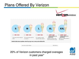
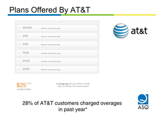
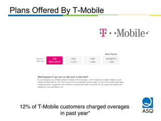
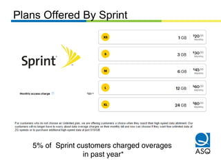
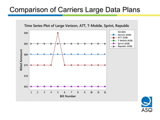
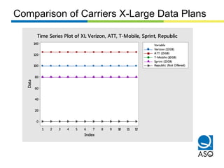
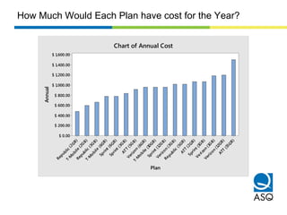
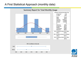
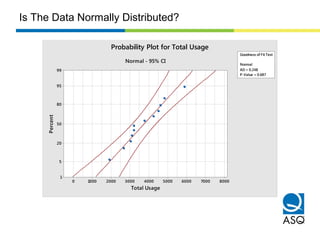
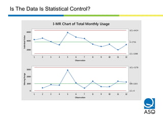
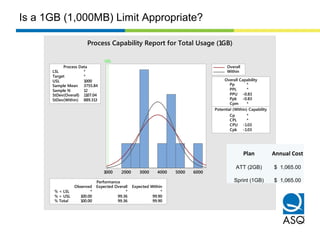
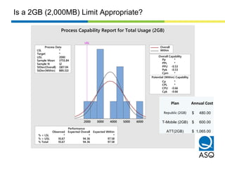
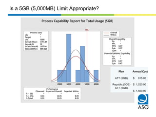
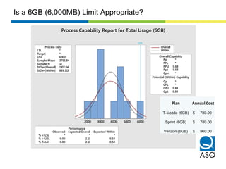
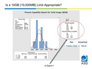
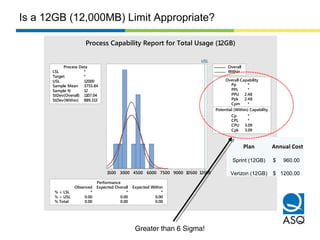
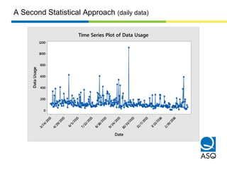
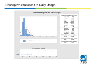
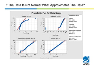
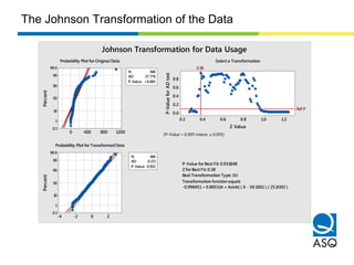
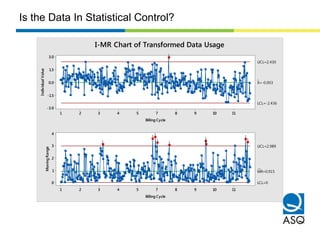
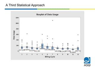
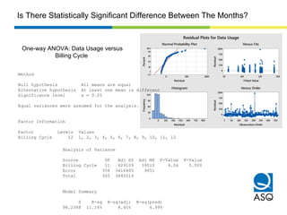
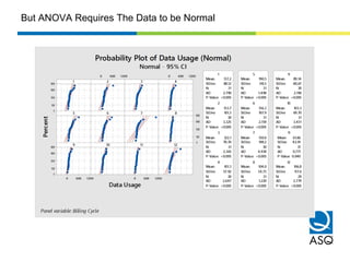
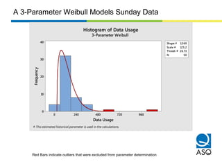
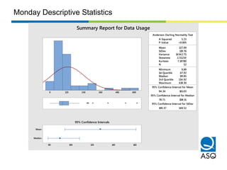
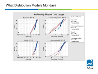
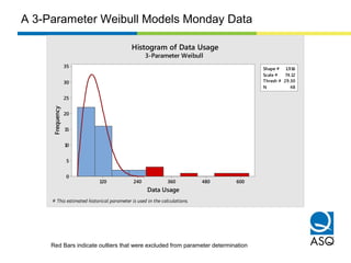
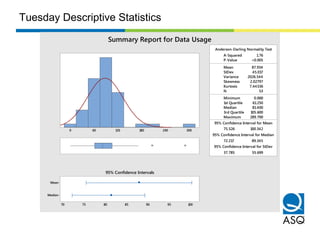
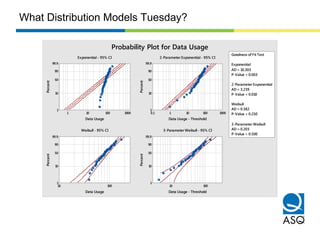
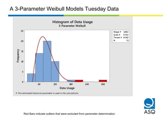
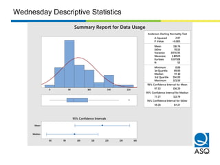
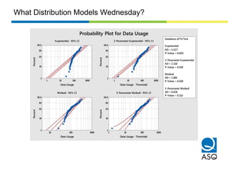
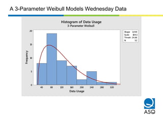
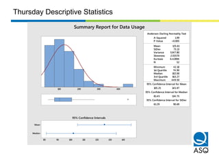
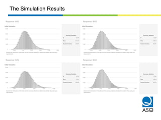
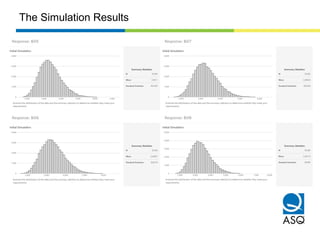
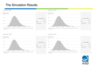
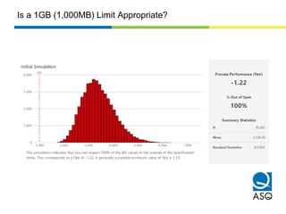
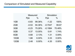
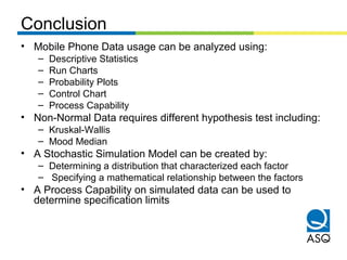
A Six Sigma Analysis of Mobile Data
Usage
2016 WCQI
Session W10
Brandon Theiss, PE
Brandon.Theiss@gmail.com
Motivation
Is my current mobile data plan with Republic Wireless
Optimal Given my data usage?
Learning Objectives
• Apply the Six Sigma Methodology to Non
Traditional Applications
• Utilize Monte Carlo simulations to make
predictions
• Utilize Non Parametric Hypothesis testing
• Utilize Process Capability to determine
specification limitations for non-normal data
4 Major Mobile Phone Carriers
Plans Offered By Verizon
20% of Verizon customers charged overages
in past year*
Plans Offered By AT&T
28% of AT&T customers charged overages
in past year*
Plans Offered By T-Mobile
12% of T-Mobile customers charged overages
in past year*
5% of Sprint customers charged overages
in past year*
Plans Offered By Sprint
Plans Offered By Republic Wireless
121110987654321
12000
10000
8000
6000
4000
2000
0
Bill Number
TotalUsage
1000
2000
3000
5000
6000
10000
12000
3095.80
1911.60
3203.80
2674.30
3224.90
4517.40
4846.80
5905.40
3039.10
3784.20
4612.40
4254.40
Chart of Total Data Usage
The Data Set
Data was collected from March 23, 2015
Through March 24, 2016
121110987654321
$130
$120
$110
$100
$90
$80
$70
$60
$50
$40
Bill Number
BilledAmmount
Verizon (1GB)
ATT (2GB)
T-Mobile (2GB)
Sprint (1GB)
Republic (2GB)
Variable
Time Series Plot of Small Verizon, ATT, T-Mobile, Sprint, Republic
Comparison of Carriers Small Data Plans
Data Speed Potentially Decreased
121110987654321
$120
$110
$100
$90
$80
$70
$60
$50
Bill Number
BilledAmmount
Verizon (3GB)
ATT (2GB)
T-Mobile (2GB)
Sprint (3GB)
Republic (3GB)
Variable
Time Series Plot of MediumVerizon, ATT, T-Mobile, Sprint, Republic
Comparison of Carriers Medium Data Plans
Data Speed Potentially Decreased
121110987654321
$90
$85
$80
$75
$70
$65
Bill Number
BilledAmmount
Verizon (6GB)
ATT (5GB)
T-Mobile (6GB)
Sprint (6GB)
Republic (5GB)
Variable
Time Series Plot of Large Verizon, ATT, T-Mobile, Sprint, Republic
Comparison of Carriers Large Data Plans
Comparison of Carriers X-Large Data Plans
121110987654321
140
120
100
80
60
40
20
0
Index
Data
Verizon (12GB)
ATT (15GB)
T-Mobile (10GB)
Sprint (12GB)
Republic (Not Offered)
Variable
Time Series Plot of XL Verizon, ATT, T-Mobile, Sprint, Republic
ATT
(15G
B)
Verizon
(12G
B)
Verizon
(1G
B)
Sprint (1G
B)
ATT
(2G
B)
Republic
(5G
B)
Verizon
(3G
B)
Sprint (12G
B)
T-M
obile
(10G
B)
Verizon
(6G
B)
ATT
(5G
B)
Sprint (3G
B)
Sprint (6G
B)
T-M
obile
(6G
B)
Republic
(3G
B)
T-M
obile
(2G
B)
Republic
(2G
B)
$ 1,600.00
$ 1,400.00
$ 1,200.00
$ 1,000.00
$ 800.00
$ 600.00
$ 400.00
$ 200.00
$ 0.00
Plan
Annual Chart of Annual Cost
How Much Would Each Plan have cost for the Year?
1st Quartile 3053.3
Median 3504.6
3rd Quartile 4588.6
Maximum 5905.4
3052.5 4459.2
3054.0 4587.4
784.2 1879.6
A-Squared 0.25
P-Value 0.687
Mean 3755.8
StDev 1107.0
Variance 1225527.2
Skewness 0.314666
Kurtosis -0.123559
N 12
Minimum 1911.6
Anderson-Darling Normality Test
95% Confidence Interval for Mean
95% Confidence Interval for Median
95% Confidence Interval for StDev
60005000400030002000
Median
Mean
4500425040003750350032503000
95% Confidence Intervals
Summary Report for Total Monthly Usage
A First Statistical Approach (monthly data)
800070006000500040003000200010000
99
95
80
50
20
5
1
Total Usage
Percent
Goodness of Fit Test
Normal
AD = 0.248
P-Value = 0.687
Probability Plot for Total Usage
Normal - 95% CI
Is The Data Normally Distributed?
121110987654321
6000
4000
2000
Observation
IndividualValue
_
X=3756
UCL=6424
LCL=1088
121110987654321
3000
2000
1000
0
Observation
MovingRange
__
MR=1003
UCL=3278
LCL=0
I-MR Chart of Total Monthly Usage
Is The Data Is Statistical Control?
600050004000300020001000
LSL *
Target *
USL 1000
Sample Mean 3755.84
Sample N 12
StDev(Overall) 1107.04
StDev(Within) 889.313
Process Data
Pp *
PPL *
PPU -0.83
Ppk -0.83
Cpm *
Cp *
CPL *
CPU -1.03
Cpk -1.03
Potential (Within) Capability
Overall Capability
% < LSL * * *
% > USL 100.00 99.36 99.90
% Total 100.00 99.36 99.90
Observed Expected Overall Expected Within
Performance
USL
Overall
Within
Process Capability Report for Total Usage (1GB)
Plan Annual Cost
ATT (2GB) $ 1,065.00
Sprint (1GB) $ 1,065.00
Is a 1GB (1,000MB) Limit Appropriate?
60005000400030002000
LSL *
Target *
USL 2000
Sample Mean 3755.84
Sample N 12
StDev(Overall) 1107.04
StDev(Within) 889.313
Process Data
Pp *
PPL *
PPU -0.53
Ppk -0.53
Cpm *
Cp *
CPL *
CPU -0.66
Cpk -0.66
Potential (Within) Capability
Overall Capability
% < LSL * * *
% > USL 91.67 94.36 97.58
% Total 91.67 94.36 97.58
Observed Expected Overall Expected Within
Performance
USL
Overall
Within
Process Capability Report for Total Usage (2GB)
Is a 2GB (2,000MB) Limit Appropriate?
Plan Annual Cost
Republic (2GB) $ 480.00
T-Mobile (2GB) $ 600.00
ATT(2GB) $ 1,065.00
60005000400030002000
LSL *
Target *
USL 3000
Sample Mean 3755.84
Sample N 12
StDev(Overall) 1107.04
StDev(Within) 889.313
Process Data
Pp *
PPL *
PPU -0.23
Ppk -0.23
Cpm *
Cp *
CPL *
CPU -0.28
Cpk -0.28
Potential (Within) Capability
Overall Capability
% < LSL * * *
% > USL 83.33 75.26 80.23
% Total 83.33 75.26 80.23
Observed Expected Overall Expected Within
Performance
USL
Overall
Within
Process Capability Report for Total Usage (3GB)
Plan Annual Cost
Republic (3GB) $ 660.00
Sprint (3GB) $ 840.00
Verizon (3GB) $ 1,020.00
Is a 3GB (3,000MB) Limit Appropriate?
60005000400030002000
LSL *
Target *
USL 5000
Sample Mean 3755.84
Sample N 12
StDev(Overall) 1107.04
StDev(Within) 889.313
Process Data
Pp *
PPL *
PPU 0.37
Ppk 0.37
Cpm *
Cp *
CPL *
CPU 0.47
Cpk 0.47
Potential (Within) Capability
Overall Capability
% < LSL * * *
% > USL 8.33 13.05 8.09
% Total 8.33 13.05 8.09
Observed Expected Overall Expected Within
Performance
USL
Overall
Within
Process Capability Report for Total Usage (5GB)
Plan Annual Cost
ATT (5GB) $ 915.00
Republic (5GB) $ 1,020.00
ATT (5GB)
$ 1,500.00
Is a 5GB (5,000MB) Limit Appropriate?
60005000400030002000
LSL *
Target *
USL 6000
Sample Mean 3755.84
Sample N 12
StDev(Overall) 1107.04
StDev(Within) 889.313
Process Data
Pp *
PPL *
PPU 0.68
Ppk 0.68
Cpm *
Cp *
CPL *
CPU 0.84
Cpk 0.84
Potential (Within) Capability
Overall Capability
% < LSL * * *
% > USL 0.00 2.13 0.58
% Total 0.00 2.13 0.58
Observed Expected Overall Expected Within
Performance
USL
Overall
Within
Process Capability Report for Total Usage (6GB)
Plan Annual Cost
T-Mobile (6GB) $ 780.00
Sprint (6GB) $ 780.00
Verizon (6GB) $ 960.00
Is a 6GB (6,000MB) Limit Appropriate?
900075006000450030001500
LSL *
Target *
USL 10000
Sample Mean 3755.84
Sample N 12
StDev(Overall) 1107.04
StDev(Within) 889.313
Process Data
Pp *
PPL *
PPU 1.88
Ppk 1.88
Cpm *
Cp *
CPL *
CPU 2.34
Cpk 2.34
Potential (Within) Capability
Overall Capability
% < LSL * * *
% > USL 0.00 0.00 0.00
% Total 0.00 0.00 0.00
Observed Expected Overall Expected Within
Performance
USL
Overall
Within
Process Capability Report for Total Usage (10GB)
Plan Annual Cost
T-Mobile (10GB) $ 960.00
Is a 10GB (10,000MB) Limit Appropriate?
~6 Sigma !
1200010500900075006000450030001500
LSL *
Target *
USL 12000
Sample Mean 3755.84
Sample N 12
StDev(Overall) 1107.04
StDev(Within) 889.313
Process Data
Pp *
PPL *
PPU 2.48
Ppk 2.48
Cpm *
Cp *
CPL *
CPU 3.09
Cpk 3.09
Potential (Within) Capability
Overall Capability
% < LSL * * *
% > USL 0.00 0.00 0.00
% Total 0.00 0.00 0.00
Observed Expected Overall Expected Within
Performance
USL
Overall
Within
Process Capability Report for Total Usage (12GB)
Plan Annual Cost
Sprint (12GB) $ 960.00
Verizon (12GB) $ 1200.00
Is a 12GB (12,000MB) Limit Appropriate?
Greater than 6 Sigma!
2/19/2016
1/13/2016
12/7/2015
10/31/2015
9/24/2015
8/18/2015
7/12/2015
6/5/2015
4/29/2015
3/24/2015
1200
1000
800
600
400
200
0
Date
DataUsage Time Series Plot of Data Usage
A Second Statistical Approach (daily data)
1st Quartile 69.13
Median 96.70
3rd Quartile 138.00
Maximum 1100.00
112.59 133.69
88.25 102.97
95.71 110.67
A-Squared 27.78
P-Value <0.005
Mean 123.14
StDev 102.64
Variance 10535.65
Skewness 3.9407
Kurtosis 26.1682
N 366
Minimum 0.00
Anderson-Darling Normality Test
95% Confidence Interval for Mean
95% Confidence Interval for Median
95% Confidence Interval for StDev
10008006004002000
Median
Mean
14013012011010090
95% Confidence Intervals
Summary Report for Data Usage
Descriptive Statistics On Daily Usage
12008004000
99.9
99
90
50
10
1
0.1
Data Usage
Percent
10000
1000
100101
0.1
0.01
0.001
0.0001
99.9
99
90
50
10
1
0.1
Data Usage
Percent
100010010
99.9
99
90
50
10
1
0.1
Data Usage - Threshold
Percent
20-2-4
99.9
99
90
50
10
1
0.1
Data Usage
Percent
3-Parameter Loglogistic
AD = 1.975
P-Value = *
Johnson Transformation
AD = 0.171
P-Value = 0.932
Goodness of Fit Test
Logistic
AD = 13.251
P-Value < 0.005
Loglogistic
AD = 9.501
P-Value < 0.005
After Johnson transformation
Probability Plot for Data Usage
Logistic - 95% CI Loglogistic - 95% CI
3-Parameter Loglogistic - 95% CI Normal - 95% CI
If The Data Is Not Normal What Approximates The Data?
12008004000
99.9
99
90
50
10
1
0.1
N 366
AD 27.776
P-Value <0.005
Percent
20-2-4
99.9
99
90
50
10
1
0.1
N 366
AD 0.171
P-Value 0.932
Percent
1.21.00.80.60.40.2
0.8
0.6
0.4
0.2
0.0
Z Value
P-ValueforADtest
0.38
Ref P
P-Value for Best Fit: 0.931848
Z for Best Fit: 0.38
Best Transformation Type: SU
Transformation function equals
-0.996951+ 0.885314 × Asinh( ( X - 59.1002 ) / 25.8392 )
Probability Plot for Original Data
Probability Plot for Transformed Data
Select a Transformation
(P-Value = 0.005 means ≤ 0.005)
Johnson Transformation for Data Usage
The Johnson Transformation of the Data
111098754321
3.0
1.5
0.0
-1.5
-3.0
Billing Cycle
IndividualValue
_
X=-0.003
UCL=2.430
LCL=-2.436
111098754321
4
3
2
1
0
Billing Cycle
MovingRange
__
MR=0.915
UCL=2.989
LCL=0
1
1
1
1
1
1
1
1
1
1
I-MR Chart of Transformed Data Usage
Is the Data In Statistical Control?
121110987654321
1200
1000
800
600
400
200
0
Billing Cycle
DataUsage
106.752
61.6645
103.34889.1433104.029
150.58156.348
190.497
101.303122.071
153.747137.239
Boxplot of Data Usage
A Third Statistical Approach
10005000
99.9
99
90
50
10
1
0.1
Residual
Percent
20015010050
1000
750
500
250
0
Fitted Value
Residual
9007506004503001500
120
90
60
30
0
Residual
Frequency
350300250200150100501
1000
750
500
250
0
Observation Order
Residual
Normal Probability Plot Versus Fits
Histogram Versus Order
Residual Plots for Data Usage
Analysis of Variance
Source DF Adj SS Adj MS F-Value P-Value
Billing Cycle 11 429109 39010 4.04 0.000
Error 354 3416405 9651
Total 365 3845514
Model Summary
S R-sq R-sq(adj) R-sq(pred)
98.2388 11.16% 8.40% 4.99%
Method
Null hypothesis All means are equal
Alternative hypothesis At least one mean is different
Significance level α = 0.05
Equal variances were assumed for the analysis.
Factor Information
Factor Levels Values
Billing Cycle 12 1, 2, 3, 4, 5, 6, 7, 8, 9, 10, 11, 12
One-way ANOVA: Data Usage versus
Billing Cycle
Is There Statistically Significant Difference Between The Months?
But ANOVA Requires The Data to be Normal
Kruskal-Wallis Test: Data Usage versus Billing Cycle
Kruskal-Wallis Test on Data Usage
Billing
Cycle N Median Ave Rank Z
1 31 108.80 217.0 1.84
2 30 130.50 249.8 3.58
3 31 88.40 187.4 0.21
4 30 85.60 160.9 -1.22
5 31 137.90 265.5 4.51
6 31 129.40 234.7 2.82
7 30 88.15 182.3 -0.07
8 31 93.80 187.9 0.24
9 30 75.70 135.9 -2.57
10 31 75.00 148.9 -1.90
11 31 62.50 86.3 -5.35
12 29 73.20 142.6 -2.17
Overall 366 183.5
H = 82.19 DF = 11 P = 0.000
H = 82.19 DF = 11 P = 0.000 (adjusted for
ties)
A First Non-Parametric Approach
20
10
0
1050
900
750
600
450
300
150
0 1050
900
750
600
450
300
150
0
20
10
0
1050
900
750
600
450
300
1500
20
10
0
1050
900
750
600
450
300
1500
1
Data Usage
Frequency
2 3 4
5 6 7 8
9 10 11 12
Histogram of Data Usage
Panel variable: Billing Cycle
Kruskal-Wallis Test Requires
The Distributions To Have Similar Shapes
Mood Median Test: Data Usage versus Billing Cycle
Mood median test for Data Usage
Chi-Square = 70.53 DF = 11 P = 0.000
Billing Individual 95.0% CIs
Cycle N≤ N> Median Q3-Q1 --+---------+---------+---------
+----
1 10 21 109 68 (*--)
2 4 26 131 45 (-*---)
3 17 14 88 59 (-*-----)
4 19 11 86 46 (-*-)
5 5 26 138 156 (-----*---------------)
6 8 23 129 81 (----*----)
7 16 14 88 78 (--*-----)
8 17 14 94 44 (-*-)
9 21 9 76 44 (-*--)
10 22 9 75 46 (-*-)
11 26 5 63 36 (-*-)
12 18 11 73 83 (--*-----)
--+---------+---------+---------
+----
60 120 180 240
Overall median = 97
A Second Non-Parametric Approach
A Fourth Statistical Approach
SaturdayFridayThursdayWednesdayTuesdayMondaySunday
1200
1000
800
600
400
200
0
Day Of Week
DataUsage
124.35117.36125.612116.7687.934
127.687163.094
Boxplot of Data Usage
A Fifth Statistical Approach (by days of the week)
20
10
0
10509007506004503001500
10509007506004503001500
20
10
0
10509007506004503001500
20
10
0
Sunday
Data Usage
Frequency
Monday Tuesday
Wednesday Thursday Friday
Saturday
Histogram of Data Usage
Panel variable: Day Of Week
What Do The Distributions Of Each Day Look Like?
SUNDAY
1st Quartile 74.32
Median 120.15
3rd Quartile 197.35
Maximum 1100.00
115.83 210.36
84.71 152.41
142.27 210.53
A-Squared 4.65
P-Value <0.005
Mean 163.09
StDev 169.77
Variance 28821.13
Skewness 3.7420
Kurtosis 18.3156
N 52
Minimum 0.00
Anderson-Darling Normality Test
95% Confidence Interval for Mean
95% Confidence Interval for Median
95% Confidence Interval for StDev
9607204802400
Median
Mean
225200175150125100
95% Confidence Intervals
Summary Report for Data Usage
Sunday Descriptive Statistics
Weibull
AD = 0.728
P-Value = 0.053
3-Parameter Weibull
AD = 0.355
P-Value = 0.475
Goodness of Fit Test
Exponential
AD = 4.176
P-Value < 0.003
2-Parameter Exponential
AD = 1.614
P-Value = 0.017
1000100101
99.9
90
50
10
1
Data Usage
Percent
1000100101
99.9
90
50
10
1
Data Usage - Threshold
Percent
100010010
99.9
90
50
10
1
Data Usage
Percent
1000100101
99.9
90
50
10
1
Data Usage - Threshold
Percent
Probability Plot for Data Usage
Exponential - 95% CI 2-Parameter Exponential - 95% CI
Weibull - 95% CI 3-Parameter Weibull - 95% CI
What Distribution Models Sunday?
9607204802400
40
30
20
10
0
Shape # 1.369
Scale # 125.2
Thresh # 26.73
N 50
Data Usage
Frequency
Histogram of Data Usage
3-Parameter Weibull
# This estimated historical parameter is used in the calculations.
A 3-Parameter Weibull Models Sunday Data
Red Bars indicate outliers that were excluded from parameter determination
MONDAY
1st Quartile 67.92
Median 89.85
3rd Quartile 134.92
Maximum 619.30
94.34 161.03
78.71 108.15
100.37 148.52
A-Squared 5.23
P-Value <0.005
Mean 127.69
StDev 119.76
Variance 14342.75
Skewness 2.55234
Kurtosis 7.19780
N 52
Minimum 0.00
Anderson-Darling Normality Test
95% Confidence Interval for Mean
95% Confidence Interval for Median
95% Confidence Interval for StDev
6004803602401200
Median
Mean
16014012010080
95% Confidence Intervals
Summary Report for Data Usage
Monday Descriptive Statistics
10001001010.10.010.0010.0001
90
50
10
1
Data Usage
Percent
1000100101
90
50
10
1
Data Usage - Threshold
Percent
10001001010.10.010.0010.0001
90
50
10
1
Data Usage
Percent
10010
90
50
10
1
Data Usage - Threshold
Percent
Weibull
AD = 2.383
P-Value < 0.010
3-Parameter Weibull
AD = 0.398
P-Value = 0.342
Goodness of Fit Test
Exponential
AD = 6.080
P-Value < 0.003
2-Parameter Exponential
AD = 6.124
P-Value < 0.010
Probability Plot for Data Usage
Exponential - 95% CI 2-Parameter Exponential - 95% CI
Weibull - 95% CI 3-Parameter Weibull - 95% CI
What Distribution Models Monday?
600480360240120
35
30
25
20
15
10
5
0
Shape # 1.916
Scale # 74.12
Thresh # 29.30
N 48
Data Usage
Frequency
Histogram of Data Usage
3-Parameter Weibull
# This estimated historical parameter is used in the calculations.
A 3-Parameter Weibull Models Monday Data
Red Bars indicate outliers that were excluded from parameter determination
TUESDAY
1st Quartile 61.250
Median 81.400
3rd Quartile 105.600
Maximum 289.700
75.526 100.342
72.217 89.345
37.785 55.699
A-Squared 1.76
P-Value <0.005
Mean 87.934
StDev 45.017
Variance 2026.544
Skewness 2.02797
Kurtosis 7.44336
N 53
Minimum 0.000
Anderson-Darling Normality Test
95% Confidence Interval for Mean
95% Confidence Interval for Median
95% Confidence Interval for StDev
300240180120600
Median
Mean
100959085807570
95% Confidence Intervals
Summary Report for Data Usage
Tuesday Descriptive Statistics
Weibull
AD = 0.382
P-Value > 0.250
3-Parameter Weibull
AD = 0.203
P-Value > 0.500
Goodness of Fit Test
Exponential
AD = 10.303
P-Value < 0.003
2-Parameter Exponential
AD = 3.239
P-Value < 0.010
1000100101
99.9
90
50
10
1
Data Usage
Percent
10001001010.1
99.9
90
50
10
1
Data Usage - Threshold
Percent
10010
99.9
90
50
10
1
Data Usage
Percent
10010
99.9
90
50
10
1
Data Usage - Threshold
Percent
Probability Plot for Data Usage
Exponential - 95% CI 2-Parameter Exponential - 95% CI
Weibull - 95% CI 3-Parameter Weibull - 95% CI
What Distribution Models Tuesday?
30024018012060
25
20
15
10
5
0
Shape # 1.882
Scale # 57.02
Thresh # 34.60
N 51
Data Usage
Frequency
Histogram of Data Usage
3-Parameter Weibull
# This estimated historical parameter is used in the calculations.
A 3-Parameter Weibull Models Tuesday Data
Red Bars indicate outliers that were excluded from parameter determination
WEDNESDAY
1st Quartile 69.00
Median 97.10
3rd Quartile 154.00
Maximum 321.50
97.32 136.20
77.27 113.79
59.20 87.27
A-Squared 2.07
P-Value <0.005
Mean 116.76
StDev 70.53
Variance 4974.95
Skewness 1.10549
Kurtosis 0.67508
N 53
Minimum 0.00
Anderson-Darling Normality Test
95% Confidence Interval for Mean
95% Confidence Interval for Median
95% Confidence Interval for StDev
320240160800
Median
Mean
1401301201101009080
95% Confidence Intervals
Summary Report for Data Usage
Wednesday Descriptive Statistics
Weibull
AD = 1.186
P-Value < 0.010
3-Parameter Weibull
AD = 0.618
P-Value = 0.113
Goodness of Fit Test
Exponential
AD = 5.427
P-Value < 0.003
2-Parameter Exponential
AD = 2.310
P-Value < 0.010
1000100101
99.9
90
50
10
1
Data Usage
Percent
1000100101
99.9
90
50
10
1
Data Usage - Threshold
Percent
100010010
99.9
90
50
10
1
Data Usage
Percent
1000100101
99.9
90
50
10
1
Data Usage - Threshold
Percent
Probability Plot for Data Usage
Exponential - 95% CI 2-Parameter Exponential - 95% CI
Weibull - 95% CI 3-Parameter Weibull - 95% CI
What Distribution Models Wednesday?
3202802402001601208040
20
15
10
5
0
Shape 1.430
Scale 104.1
Thresh 24.66
N 52
Data Usage
Frequency
Histogram of Data Usage
3-Parameter Weibull
A 3-Parameter Weibull Models Wednesday Data
THURSDAY
1st Quartile 74.90
Median 102.00
3rd Quartile 163.27
Maximum 449.50
105.25 145.97
81.45 134.75
61.29 90.69
A-Squared 1.99
P-Value <0.005
Mean 125.61
StDev 73.13
Variance 5347.80
Skewness 2.03570
Kurtosis 6.42894
N 52
Minimum 42.10
Anderson-Darling Normality Test
95% Confidence Interval for Mean
95% Confidence Interval for Median
95% Confidence Interval for StDev
400300200100
Median
Mean
1401301201101009080
95% Confidence Intervals
Summary Report for Data Usage
Thursday Descriptive Statistics
Weibull
AD = 0.904
P-Value = 0.020
3-Parameter Weibull
AD = 0.324
P-Value > 0.500
Goodness of Fit Test
Exponential
AD = 6.944
P-Value < 0.003
2-Parameter Exponential
AD = 1.454
P-Value = 0.025
1000100101
99.9
90
50
10
1
Data Usage
Percent
1000100101
99.9
90
50
10
1
Data Usage - Threshold
Percent
100010010
99.9
90
50
10
1
Data Usage
Percent
1000100101
99.9
90
50
10
1
Data Usage - Threshold
Percent
Probability Plot for Data Usage
Exponential - 95% CI 2-Parameter Exponential - 95% CI
Weibull - 95% CI 3-Parameter Weibull - 95% CI
What Distribution Models Thursday?
400300200100
25
20
15
10
5
0
Shape # 1.364
Scale # 85.54
Thresh # 40.89
N 52
Data Usage
Frequency
Histogram of Data Usage
3-Parameter Weibull
# This estimated historical parameter is used in the calculations.
A 3-Parameter Weibull Models Thursday Data
Red Bars indicate outliers that were excluded from parameter determination
FRIDAY
1st Quartile 67.70
Median 100.95
3rd Quartile 122.95
Maximum 435.30
94.58 140.14
84.26 105.70
68.58 101.49
A-Squared 4.30
P-Value <0.005
Mean 117.36
StDev 81.84
Variance 6697.42
Skewness 2.21566
Kurtosis 5.35910
N 52
Minimum 10.70
Anderson-Darling Normality Test
95% Confidence Interval for Mean
95% Confidence Interval for Median
95% Confidence Interval for StDev
4003002001000
Median
Mean
1401301201101009080
95% Confidence Intervals
Summary Report for Data Usage
Friday Descriptive Statistics
Weibull
AD = 0.607
P-Value = 0.111
3-Parameter Weibull
AD = 0.392
P-Value = 0.404
Goodness of Fit Test
Exponential
AD = 9.088
P-Value < 0.003
2-Parameter Exponential
AD = 2.477
P-Value < 0.010
1000100101
90
50
10
1
Data Usage
Percent
10001001010.1
90
50
10
1
Data Usage - Threshold
Percent
10010
90
50
10
1
Data Usage
Percent
10010
90
50
10
1
Data Usage - Threshold
Percent
Probability Plot for Data Usage
Exponential - 95% CI 2-Parameter Exponential - 95% CI
Weibull - 95% CI 3-Parameter Weibull - 95% CI
What Distribution Models Friday?
400300200100
35
30
25
20
15
10
5
0
Shape # 1.670
Scale # 61.32
Thresh # 39.17
N 51
Data Usage
Frequency
Histogram of Data Usage
3-Parameter Weibull
# This estimated historical parameter is used in the calculations.
A 3-Parameter Weibull Models Friday Data
Red Bars indicate outliers that were excluded from parameter determination
SATURDAY
1st Quartile 69.73
Median 101.85
3rd Quartile 137.40
Maximum 597.70
96.46 152.24
82.46 121.30
83.94 124.22
A-Squared 4.52
P-Value <0.005
Mean 124.35
StDev 100.17
Variance 10033.47
Skewness 2.79744
Kurtosis 9.97571
N 52
Minimum 0.00
Anderson-Darling Normality Test
95% Confidence Interval for Mean
95% Confidence Interval for Median
95% Confidence Interval for StDev
6004803602401200
Median
Mean
16014012010080
95% Confidence Intervals
Summary Report for Data Usage
Saturday Descriptive Statistics
Weibull
AD = 1.262
P-Value < 0.010
3-Parameter Weibull
AD = 0.441
P-Value = 0.310
Goodness of Fit Test
Exponential
AD = 7.494
P-Value < 0.003
2-Parameter Exponential
AD = 1.317
P-Value = 0.037
1000100101
90
50
10
1
Data Usage
Percent
1000100101
90
50
10
1
Data Usage - Threshold
Percent
10010
90
50
10
1
Data Usage
Percent
1000100101
90
50
10
1
Data Usage - Threshold
Percent
Probability Plot for Data Usage
Exponential - 95% CI 2-Parameter Exponential - 95% CI
Weibull - 95% CI 3-Parameter Weibull - 95% CI
What Distribution Models Saturday?
600480360240120
35
30
25
20
15
10
5
0
Shape # 1.246
Scale # 69.33
Thresh # 44.41
N 50
Data Usage
Frequency
Histogram of Data Usage
3-Parameter Weibull
# This estimated historical parameter is used in the calculations.
A 3-Parameter Weibull Models Saturday Data
Red Bars indicate outliers that were excluded from parameter determination
THE SIMULATION
The Simulation Equation
Sunday Monday Tuesday Wednesday Thursday Friday Saturday
Sunday Monday Tuesday Wednesday Thursday
Tuesday Wednesday Thursday Friday Saturday
+
+
+
+
+
+
+
+
+
+
+
+
+
+
+
+
+
+
+
+
+
+
+
+
+
+
+
+
+ +=Bill 1
Sunday Monday Tuesday Wednesday Thursday Friday Saturday Total
Bill1 4 4 5 5 5 4 4 31
Bill2 4 4 4 4 4 5 5 30
Bill3 5 5 5 4 4 4 4 31
Bill4 4 4 4 5 5 4 4 30
Bill5 5 4 4 4 4 5 5 31
Bill6 4 5 5 5 4 4 4 31
Bill7 4 4 4 4 5 5 4 30
Bill8 5 5 4 4 4 4 5 31
Bill9 4 4 5 5 4 4 4 30
Bill10 4 4 4 4 5 5 5 31
Bill11 5 5 5 4 4 4 4 31
Bill12 4 4 4 5 4 4 4 29
The Simulation Parameters
The Simulation Results
ASSESSING CAPABILITY
FROM SIMULATION RESULTS
Is a 1GB (1,000MB) Limit Appropriate?
Is a 2GB (2,000MB) Limit Appropriate?
Is a 3GB (3,000MB) Limit Appropriate?
Is a 4GB (4,000MB) Limit Appropriate?
Is a 5GB (5,000MB) Limit Appropriate?
Is a 6GB (6,000MB) Limit Appropriate?
Is a 10GB (10,000MB) Limit Appropriate?
Is a 12GB (12,000MB) Limit Appropriate?
Data Usage <1 1-2 2-3 3-4 4-5 5-6 >6
Expected
Monthly
Charge0.000% 0.330% 29.190% 52.890% 15.850% 1.650% 0.090%
Sprint (1GB) $ 40.00 $ 0.05 $ 4.38 $ 7.93 $ 2.38 $ 0.25 $ 0.01 $ 55.00
Sprint (3GB) $ 50.00 $ 7.93 $ 2.38 $ 0.25 $ 0.01 $ 60.57
Sprint (6GB) $ 65.00 $ 65.00
VZ (1Gb) $ 50.00 $ 0.05 $ 4.38 $ 7.93 $ 2.38 $ 0.25 $ 0.01 $ 65.00
ATT (2GB) $ 55.00 $ 4.38 $ 7.93 $ 2.38 $ 0.25 $ 0.01 $ 69.95
ATT (5GB) $ 75.00 $ 0.25 $ 0.01 $ 75.26
VZ (3GB) $ 65.00 $ 7.93 $ 2.38 $ 0.25 $ 0.01 $ 75.57
Sprint (12GB) $ 80.00 $ 80.00
VZ (6GB) $ 80.00 $ 0.01 $ 80.01
VZ(12GB) $ 100.00 $ 100.00
ATT (15GB) $ 125.00 $ 125.00
Plan Selection Based on Simulation
Measured Simulation
Ppk % Ppk %
1GB -0.83 99.36% -1.22 100%
2GB -0.53 94.36% -0.7047 99.67
3GB -0.23 75.26% -0.1984 70.48%
5GB 0.37 13.05% 0.81 1.74%
6GB 0.68 2.13% 1.31 0.09%
10GB 1.88 0.00% 3.33 0.00%
12GB 2.48 0.00% 4.35 0.00%
Comparison of Simulated and Measured Capability
Conclusion
• Mobile Phone Data usage can be analyzed using:
– Descriptive Statistics
– Run Charts
– Probability Plots
– Control Chart
– Process Capability
• Non-Normal Data requires different hypothesis test including:
– Kruskal-Wallis
– Mood Median
• A Stochastic Simulation Model can be created by:
– Determining a distribution that characterized each factor
– Specifying a mathematical relationship between the factors
• A Process Capability on simulated data can be used to
determine specification limits
Questions?
Contact Information:
Brandon R. Theiss, PE
Rutgers School of Law- Camden
Brandon.Theiss@Rutgers.edu

A Six Sigma Analysis of Mobile Data Usage

  • 1.
    A Six SigmaAnalysis of Mobile Data Usage 2016 WCQI Session W10 Brandon Theiss, PE Brandon.Theiss@gmail.com
  • 2.
    Motivation Is my currentmobile data plan with Republic Wireless Optimal Given my data usage?
  • 3.
    Learning Objectives • Applythe Six Sigma Methodology to Non Traditional Applications • Utilize Monte Carlo simulations to make predictions • Utilize Non Parametric Hypothesis testing • Utilize Process Capability to determine specification limitations for non-normal data
  • 4.
    4 Major MobilePhone Carriers
  • 5.
    Plans Offered ByVerizon 20% of Verizon customers charged overages in past year*
  • 6.
    Plans Offered ByAT&T 28% of AT&T customers charged overages in past year*
  • 7.
    Plans Offered ByT-Mobile 12% of T-Mobile customers charged overages in past year*
  • 8.
    5% of Sprintcustomers charged overages in past year* Plans Offered By Sprint
  • 9.
    Plans Offered ByRepublic Wireless
  • 10.
  • 11.
    121110987654321 $130 $120 $110 $100 $90 $80 $70 $60 $50 $40 Bill Number BilledAmmount Verizon (1GB) ATT(2GB) T-Mobile (2GB) Sprint (1GB) Republic (2GB) Variable Time Series Plot of Small Verizon, ATT, T-Mobile, Sprint, Republic Comparison of Carriers Small Data Plans Data Speed Potentially Decreased
  • 12.
    121110987654321 $120 $110 $100 $90 $80 $70 $60 $50 Bill Number BilledAmmount Verizon (3GB) ATT(2GB) T-Mobile (2GB) Sprint (3GB) Republic (3GB) Variable Time Series Plot of MediumVerizon, ATT, T-Mobile, Sprint, Republic Comparison of Carriers Medium Data Plans Data Speed Potentially Decreased
  • 13.
    121110987654321 $90 $85 $80 $75 $70 $65 Bill Number BilledAmmount Verizon (6GB) ATT(5GB) T-Mobile (6GB) Sprint (6GB) Republic (5GB) Variable Time Series Plot of Large Verizon, ATT, T-Mobile, Sprint, Republic Comparison of Carriers Large Data Plans
  • 14.
    Comparison of CarriersX-Large Data Plans 121110987654321 140 120 100 80 60 40 20 0 Index Data Verizon (12GB) ATT (15GB) T-Mobile (10GB) Sprint (12GB) Republic (Not Offered) Variable Time Series Plot of XL Verizon, ATT, T-Mobile, Sprint, Republic
  • 15.
    ATT (15G B) Verizon (12G B) Verizon (1G B) Sprint (1G B) ATT (2G B) Republic (5G B) Verizon (3G B) Sprint (12G B) T-M obile (10G B) Verizon (6G B) ATT (5G B) Sprint(3G B) Sprint (6G B) T-M obile (6G B) Republic (3G B) T-M obile (2G B) Republic (2G B) $ 1,600.00 $ 1,400.00 $ 1,200.00 $ 1,000.00 $ 800.00 $ 600.00 $ 400.00 $ 200.00 $ 0.00 Plan Annual Chart of Annual Cost How Much Would Each Plan have cost for the Year?
  • 16.
    1st Quartile 3053.3 Median3504.6 3rd Quartile 4588.6 Maximum 5905.4 3052.5 4459.2 3054.0 4587.4 784.2 1879.6 A-Squared 0.25 P-Value 0.687 Mean 3755.8 StDev 1107.0 Variance 1225527.2 Skewness 0.314666 Kurtosis -0.123559 N 12 Minimum 1911.6 Anderson-Darling Normality Test 95% Confidence Interval for Mean 95% Confidence Interval for Median 95% Confidence Interval for StDev 60005000400030002000 Median Mean 4500425040003750350032503000 95% Confidence Intervals Summary Report for Total Monthly Usage A First Statistical Approach (monthly data)
  • 17.
    800070006000500040003000200010000 99 95 80 50 20 5 1 Total Usage Percent Goodness ofFit Test Normal AD = 0.248 P-Value = 0.687 Probability Plot for Total Usage Normal - 95% CI Is The Data Normally Distributed?
  • 18.
  • 19.
    600050004000300020001000 LSL * Target * USL1000 Sample Mean 3755.84 Sample N 12 StDev(Overall) 1107.04 StDev(Within) 889.313 Process Data Pp * PPL * PPU -0.83 Ppk -0.83 Cpm * Cp * CPL * CPU -1.03 Cpk -1.03 Potential (Within) Capability Overall Capability % < LSL * * * % > USL 100.00 99.36 99.90 % Total 100.00 99.36 99.90 Observed Expected Overall Expected Within Performance USL Overall Within Process Capability Report for Total Usage (1GB) Plan Annual Cost ATT (2GB) $ 1,065.00 Sprint (1GB) $ 1,065.00 Is a 1GB (1,000MB) Limit Appropriate?
  • 20.
    60005000400030002000 LSL * Target * USL2000 Sample Mean 3755.84 Sample N 12 StDev(Overall) 1107.04 StDev(Within) 889.313 Process Data Pp * PPL * PPU -0.53 Ppk -0.53 Cpm * Cp * CPL * CPU -0.66 Cpk -0.66 Potential (Within) Capability Overall Capability % < LSL * * * % > USL 91.67 94.36 97.58 % Total 91.67 94.36 97.58 Observed Expected Overall Expected Within Performance USL Overall Within Process Capability Report for Total Usage (2GB) Is a 2GB (2,000MB) Limit Appropriate? Plan Annual Cost Republic (2GB) $ 480.00 T-Mobile (2GB) $ 600.00 ATT(2GB) $ 1,065.00
  • 21.
    60005000400030002000 LSL * Target * USL3000 Sample Mean 3755.84 Sample N 12 StDev(Overall) 1107.04 StDev(Within) 889.313 Process Data Pp * PPL * PPU -0.23 Ppk -0.23 Cpm * Cp * CPL * CPU -0.28 Cpk -0.28 Potential (Within) Capability Overall Capability % < LSL * * * % > USL 83.33 75.26 80.23 % Total 83.33 75.26 80.23 Observed Expected Overall Expected Within Performance USL Overall Within Process Capability Report for Total Usage (3GB) Plan Annual Cost Republic (3GB) $ 660.00 Sprint (3GB) $ 840.00 Verizon (3GB) $ 1,020.00 Is a 3GB (3,000MB) Limit Appropriate?
  • 22.
    60005000400030002000 LSL * Target * USL5000 Sample Mean 3755.84 Sample N 12 StDev(Overall) 1107.04 StDev(Within) 889.313 Process Data Pp * PPL * PPU 0.37 Ppk 0.37 Cpm * Cp * CPL * CPU 0.47 Cpk 0.47 Potential (Within) Capability Overall Capability % < LSL * * * % > USL 8.33 13.05 8.09 % Total 8.33 13.05 8.09 Observed Expected Overall Expected Within Performance USL Overall Within Process Capability Report for Total Usage (5GB) Plan Annual Cost ATT (5GB) $ 915.00 Republic (5GB) $ 1,020.00 ATT (5GB) $ 1,500.00 Is a 5GB (5,000MB) Limit Appropriate?
  • 23.
    60005000400030002000 LSL * Target * USL6000 Sample Mean 3755.84 Sample N 12 StDev(Overall) 1107.04 StDev(Within) 889.313 Process Data Pp * PPL * PPU 0.68 Ppk 0.68 Cpm * Cp * CPL * CPU 0.84 Cpk 0.84 Potential (Within) Capability Overall Capability % < LSL * * * % > USL 0.00 2.13 0.58 % Total 0.00 2.13 0.58 Observed Expected Overall Expected Within Performance USL Overall Within Process Capability Report for Total Usage (6GB) Plan Annual Cost T-Mobile (6GB) $ 780.00 Sprint (6GB) $ 780.00 Verizon (6GB) $ 960.00 Is a 6GB (6,000MB) Limit Appropriate?
  • 24.
    900075006000450030001500 LSL * Target * USL10000 Sample Mean 3755.84 Sample N 12 StDev(Overall) 1107.04 StDev(Within) 889.313 Process Data Pp * PPL * PPU 1.88 Ppk 1.88 Cpm * Cp * CPL * CPU 2.34 Cpk 2.34 Potential (Within) Capability Overall Capability % < LSL * * * % > USL 0.00 0.00 0.00 % Total 0.00 0.00 0.00 Observed Expected Overall Expected Within Performance USL Overall Within Process Capability Report for Total Usage (10GB) Plan Annual Cost T-Mobile (10GB) $ 960.00 Is a 10GB (10,000MB) Limit Appropriate? ~6 Sigma !
  • 25.
    1200010500900075006000450030001500 LSL * Target * USL12000 Sample Mean 3755.84 Sample N 12 StDev(Overall) 1107.04 StDev(Within) 889.313 Process Data Pp * PPL * PPU 2.48 Ppk 2.48 Cpm * Cp * CPL * CPU 3.09 Cpk 3.09 Potential (Within) Capability Overall Capability % < LSL * * * % > USL 0.00 0.00 0.00 % Total 0.00 0.00 0.00 Observed Expected Overall Expected Within Performance USL Overall Within Process Capability Report for Total Usage (12GB) Plan Annual Cost Sprint (12GB) $ 960.00 Verizon (12GB) $ 1200.00 Is a 12GB (12,000MB) Limit Appropriate? Greater than 6 Sigma!
  • 26.
  • 27.
    1st Quartile 69.13 Median96.70 3rd Quartile 138.00 Maximum 1100.00 112.59 133.69 88.25 102.97 95.71 110.67 A-Squared 27.78 P-Value <0.005 Mean 123.14 StDev 102.64 Variance 10535.65 Skewness 3.9407 Kurtosis 26.1682 N 366 Minimum 0.00 Anderson-Darling Normality Test 95% Confidence Interval for Mean 95% Confidence Interval for Median 95% Confidence Interval for StDev 10008006004002000 Median Mean 14013012011010090 95% Confidence Intervals Summary Report for Data Usage Descriptive Statistics On Daily Usage
  • 28.
    12008004000 99.9 99 90 50 10 1 0.1 Data Usage Percent 10000 1000 100101 0.1 0.01 0.001 0.0001 99.9 99 90 50 10 1 0.1 Data Usage Percent 100010010 99.9 99 90 50 10 1 0.1 DataUsage - Threshold Percent 20-2-4 99.9 99 90 50 10 1 0.1 Data Usage Percent 3-Parameter Loglogistic AD = 1.975 P-Value = * Johnson Transformation AD = 0.171 P-Value = 0.932 Goodness of Fit Test Logistic AD = 13.251 P-Value < 0.005 Loglogistic AD = 9.501 P-Value < 0.005 After Johnson transformation Probability Plot for Data Usage Logistic - 95% CI Loglogistic - 95% CI 3-Parameter Loglogistic - 95% CI Normal - 95% CI If The Data Is Not Normal What Approximates The Data?
  • 29.
    12008004000 99.9 99 90 50 10 1 0.1 N 366 AD 27.776 P-Value<0.005 Percent 20-2-4 99.9 99 90 50 10 1 0.1 N 366 AD 0.171 P-Value 0.932 Percent 1.21.00.80.60.40.2 0.8 0.6 0.4 0.2 0.0 Z Value P-ValueforADtest 0.38 Ref P P-Value for Best Fit: 0.931848 Z for Best Fit: 0.38 Best Transformation Type: SU Transformation function equals -0.996951+ 0.885314 × Asinh( ( X - 59.1002 ) / 25.8392 ) Probability Plot for Original Data Probability Plot for Transformed Data Select a Transformation (P-Value = 0.005 means ≤ 0.005) Johnson Transformation for Data Usage The Johnson Transformation of the Data
  • 30.
  • 31.
  • 32.
    10005000 99.9 99 90 50 10 1 0.1 Residual Percent 20015010050 1000 750 500 250 0 Fitted Value Residual 9007506004503001500 120 90 60 30 0 Residual Frequency 350300250200150100501 1000 750 500 250 0 Observation Order Residual NormalProbability Plot Versus Fits Histogram Versus Order Residual Plots for Data Usage Analysis of Variance Source DF Adj SS Adj MS F-Value P-Value Billing Cycle 11 429109 39010 4.04 0.000 Error 354 3416405 9651 Total 365 3845514 Model Summary S R-sq R-sq(adj) R-sq(pred) 98.2388 11.16% 8.40% 4.99% Method Null hypothesis All means are equal Alternative hypothesis At least one mean is different Significance level α = 0.05 Equal variances were assumed for the analysis. Factor Information Factor Levels Values Billing Cycle 12 1, 2, 3, 4, 5, 6, 7, 8, 9, 10, 11, 12 One-way ANOVA: Data Usage versus Billing Cycle Is There Statistically Significant Difference Between The Months?
  • 33.
    But ANOVA RequiresThe Data to be Normal
  • 34.
    Kruskal-Wallis Test: DataUsage versus Billing Cycle Kruskal-Wallis Test on Data Usage Billing Cycle N Median Ave Rank Z 1 31 108.80 217.0 1.84 2 30 130.50 249.8 3.58 3 31 88.40 187.4 0.21 4 30 85.60 160.9 -1.22 5 31 137.90 265.5 4.51 6 31 129.40 234.7 2.82 7 30 88.15 182.3 -0.07 8 31 93.80 187.9 0.24 9 30 75.70 135.9 -2.57 10 31 75.00 148.9 -1.90 11 31 62.50 86.3 -5.35 12 29 73.20 142.6 -2.17 Overall 366 183.5 H = 82.19 DF = 11 P = 0.000 H = 82.19 DF = 11 P = 0.000 (adjusted for ties) A First Non-Parametric Approach
  • 35.
    20 10 0 1050 900 750 600 450 300 150 0 1050 900 750 600 450 300 150 0 20 10 0 1050 900 750 600 450 300 1500 20 10 0 1050 900 750 600 450 300 1500 1 Data Usage Frequency 23 4 5 6 7 8 9 10 11 12 Histogram of Data Usage Panel variable: Billing Cycle Kruskal-Wallis Test Requires The Distributions To Have Similar Shapes
  • 36.
    Mood Median Test:Data Usage versus Billing Cycle Mood median test for Data Usage Chi-Square = 70.53 DF = 11 P = 0.000 Billing Individual 95.0% CIs Cycle N≤ N> Median Q3-Q1 --+---------+---------+--------- +---- 1 10 21 109 68 (*--) 2 4 26 131 45 (-*---) 3 17 14 88 59 (-*-----) 4 19 11 86 46 (-*-) 5 5 26 138 156 (-----*---------------) 6 8 23 129 81 (----*----) 7 16 14 88 78 (--*-----) 8 17 14 94 44 (-*-) 9 21 9 76 44 (-*--) 10 22 9 75 46 (-*-) 11 26 5 63 36 (-*-) 12 18 11 73 83 (--*-----) --+---------+---------+--------- +---- 60 120 180 240 Overall median = 97 A Second Non-Parametric Approach
  • 37.
  • 38.
  • 39.
    20 10 0 10509007506004503001500 10509007506004503001500 20 10 0 10509007506004503001500 20 10 0 Sunday Data Usage Frequency Monday Tuesday WednesdayThursday Friday Saturday Histogram of Data Usage Panel variable: Day Of Week What Do The Distributions Of Each Day Look Like?
  • 40.
  • 41.
    1st Quartile 74.32 Median120.15 3rd Quartile 197.35 Maximum 1100.00 115.83 210.36 84.71 152.41 142.27 210.53 A-Squared 4.65 P-Value <0.005 Mean 163.09 StDev 169.77 Variance 28821.13 Skewness 3.7420 Kurtosis 18.3156 N 52 Minimum 0.00 Anderson-Darling Normality Test 95% Confidence Interval for Mean 95% Confidence Interval for Median 95% Confidence Interval for StDev 9607204802400 Median Mean 225200175150125100 95% Confidence Intervals Summary Report for Data Usage Sunday Descriptive Statistics
  • 42.
    Weibull AD = 0.728 P-Value= 0.053 3-Parameter Weibull AD = 0.355 P-Value = 0.475 Goodness of Fit Test Exponential AD = 4.176 P-Value < 0.003 2-Parameter Exponential AD = 1.614 P-Value = 0.017 1000100101 99.9 90 50 10 1 Data Usage Percent 1000100101 99.9 90 50 10 1 Data Usage - Threshold Percent 100010010 99.9 90 50 10 1 Data Usage Percent 1000100101 99.9 90 50 10 1 Data Usage - Threshold Percent Probability Plot for Data Usage Exponential - 95% CI 2-Parameter Exponential - 95% CI Weibull - 95% CI 3-Parameter Weibull - 95% CI What Distribution Models Sunday?
  • 43.
    9607204802400 40 30 20 10 0 Shape # 1.369 Scale# 125.2 Thresh # 26.73 N 50 Data Usage Frequency Histogram of Data Usage 3-Parameter Weibull # This estimated historical parameter is used in the calculations. A 3-Parameter Weibull Models Sunday Data Red Bars indicate outliers that were excluded from parameter determination
  • 44.
  • 45.
    1st Quartile 67.92 Median89.85 3rd Quartile 134.92 Maximum 619.30 94.34 161.03 78.71 108.15 100.37 148.52 A-Squared 5.23 P-Value <0.005 Mean 127.69 StDev 119.76 Variance 14342.75 Skewness 2.55234 Kurtosis 7.19780 N 52 Minimum 0.00 Anderson-Darling Normality Test 95% Confidence Interval for Mean 95% Confidence Interval for Median 95% Confidence Interval for StDev 6004803602401200 Median Mean 16014012010080 95% Confidence Intervals Summary Report for Data Usage Monday Descriptive Statistics
  • 46.
    10001001010.10.010.0010.0001 90 50 10 1 Data Usage Percent 1000100101 90 50 10 1 Data Usage- Threshold Percent 10001001010.10.010.0010.0001 90 50 10 1 Data Usage Percent 10010 90 50 10 1 Data Usage - Threshold Percent Weibull AD = 2.383 P-Value < 0.010 3-Parameter Weibull AD = 0.398 P-Value = 0.342 Goodness of Fit Test Exponential AD = 6.080 P-Value < 0.003 2-Parameter Exponential AD = 6.124 P-Value < 0.010 Probability Plot for Data Usage Exponential - 95% CI 2-Parameter Exponential - 95% CI Weibull - 95% CI 3-Parameter Weibull - 95% CI What Distribution Models Monday?
  • 47.
    600480360240120 35 30 25 20 15 10 5 0 Shape # 1.916 Scale# 74.12 Thresh # 29.30 N 48 Data Usage Frequency Histogram of Data Usage 3-Parameter Weibull # This estimated historical parameter is used in the calculations. A 3-Parameter Weibull Models Monday Data Red Bars indicate outliers that were excluded from parameter determination
  • 48.
  • 49.
    1st Quartile 61.250 Median81.400 3rd Quartile 105.600 Maximum 289.700 75.526 100.342 72.217 89.345 37.785 55.699 A-Squared 1.76 P-Value <0.005 Mean 87.934 StDev 45.017 Variance 2026.544 Skewness 2.02797 Kurtosis 7.44336 N 53 Minimum 0.000 Anderson-Darling Normality Test 95% Confidence Interval for Mean 95% Confidence Interval for Median 95% Confidence Interval for StDev 300240180120600 Median Mean 100959085807570 95% Confidence Intervals Summary Report for Data Usage Tuesday Descriptive Statistics
  • 50.
    Weibull AD = 0.382 P-Value> 0.250 3-Parameter Weibull AD = 0.203 P-Value > 0.500 Goodness of Fit Test Exponential AD = 10.303 P-Value < 0.003 2-Parameter Exponential AD = 3.239 P-Value < 0.010 1000100101 99.9 90 50 10 1 Data Usage Percent 10001001010.1 99.9 90 50 10 1 Data Usage - Threshold Percent 10010 99.9 90 50 10 1 Data Usage Percent 10010 99.9 90 50 10 1 Data Usage - Threshold Percent Probability Plot for Data Usage Exponential - 95% CI 2-Parameter Exponential - 95% CI Weibull - 95% CI 3-Parameter Weibull - 95% CI What Distribution Models Tuesday?
  • 51.
    30024018012060 25 20 15 10 5 0 Shape # 1.882 Scale# 57.02 Thresh # 34.60 N 51 Data Usage Frequency Histogram of Data Usage 3-Parameter Weibull # This estimated historical parameter is used in the calculations. A 3-Parameter Weibull Models Tuesday Data Red Bars indicate outliers that were excluded from parameter determination
  • 52.
  • 53.
    1st Quartile 69.00 Median97.10 3rd Quartile 154.00 Maximum 321.50 97.32 136.20 77.27 113.79 59.20 87.27 A-Squared 2.07 P-Value <0.005 Mean 116.76 StDev 70.53 Variance 4974.95 Skewness 1.10549 Kurtosis 0.67508 N 53 Minimum 0.00 Anderson-Darling Normality Test 95% Confidence Interval for Mean 95% Confidence Interval for Median 95% Confidence Interval for StDev 320240160800 Median Mean 1401301201101009080 95% Confidence Intervals Summary Report for Data Usage Wednesday Descriptive Statistics
  • 54.
    Weibull AD = 1.186 P-Value< 0.010 3-Parameter Weibull AD = 0.618 P-Value = 0.113 Goodness of Fit Test Exponential AD = 5.427 P-Value < 0.003 2-Parameter Exponential AD = 2.310 P-Value < 0.010 1000100101 99.9 90 50 10 1 Data Usage Percent 1000100101 99.9 90 50 10 1 Data Usage - Threshold Percent 100010010 99.9 90 50 10 1 Data Usage Percent 1000100101 99.9 90 50 10 1 Data Usage - Threshold Percent Probability Plot for Data Usage Exponential - 95% CI 2-Parameter Exponential - 95% CI Weibull - 95% CI 3-Parameter Weibull - 95% CI What Distribution Models Wednesday?
  • 55.
    3202802402001601208040 20 15 10 5 0 Shape 1.430 Scale 104.1 Thresh24.66 N 52 Data Usage Frequency Histogram of Data Usage 3-Parameter Weibull A 3-Parameter Weibull Models Wednesday Data
  • 56.
  • 57.
    1st Quartile 74.90 Median102.00 3rd Quartile 163.27 Maximum 449.50 105.25 145.97 81.45 134.75 61.29 90.69 A-Squared 1.99 P-Value <0.005 Mean 125.61 StDev 73.13 Variance 5347.80 Skewness 2.03570 Kurtosis 6.42894 N 52 Minimum 42.10 Anderson-Darling Normality Test 95% Confidence Interval for Mean 95% Confidence Interval for Median 95% Confidence Interval for StDev 400300200100 Median Mean 1401301201101009080 95% Confidence Intervals Summary Report for Data Usage Thursday Descriptive Statistics
  • 58.
    Weibull AD = 0.904 P-Value= 0.020 3-Parameter Weibull AD = 0.324 P-Value > 0.500 Goodness of Fit Test Exponential AD = 6.944 P-Value < 0.003 2-Parameter Exponential AD = 1.454 P-Value = 0.025 1000100101 99.9 90 50 10 1 Data Usage Percent 1000100101 99.9 90 50 10 1 Data Usage - Threshold Percent 100010010 99.9 90 50 10 1 Data Usage Percent 1000100101 99.9 90 50 10 1 Data Usage - Threshold Percent Probability Plot for Data Usage Exponential - 95% CI 2-Parameter Exponential - 95% CI Weibull - 95% CI 3-Parameter Weibull - 95% CI What Distribution Models Thursday?
  • 59.
    400300200100 25 20 15 10 5 0 Shape # 1.364 Scale# 85.54 Thresh # 40.89 N 52 Data Usage Frequency Histogram of Data Usage 3-Parameter Weibull # This estimated historical parameter is used in the calculations. A 3-Parameter Weibull Models Thursday Data Red Bars indicate outliers that were excluded from parameter determination
  • 60.
  • 61.
    1st Quartile 67.70 Median100.95 3rd Quartile 122.95 Maximum 435.30 94.58 140.14 84.26 105.70 68.58 101.49 A-Squared 4.30 P-Value <0.005 Mean 117.36 StDev 81.84 Variance 6697.42 Skewness 2.21566 Kurtosis 5.35910 N 52 Minimum 10.70 Anderson-Darling Normality Test 95% Confidence Interval for Mean 95% Confidence Interval for Median 95% Confidence Interval for StDev 4003002001000 Median Mean 1401301201101009080 95% Confidence Intervals Summary Report for Data Usage Friday Descriptive Statistics
  • 62.
    Weibull AD = 0.607 P-Value= 0.111 3-Parameter Weibull AD = 0.392 P-Value = 0.404 Goodness of Fit Test Exponential AD = 9.088 P-Value < 0.003 2-Parameter Exponential AD = 2.477 P-Value < 0.010 1000100101 90 50 10 1 Data Usage Percent 10001001010.1 90 50 10 1 Data Usage - Threshold Percent 10010 90 50 10 1 Data Usage Percent 10010 90 50 10 1 Data Usage - Threshold Percent Probability Plot for Data Usage Exponential - 95% CI 2-Parameter Exponential - 95% CI Weibull - 95% CI 3-Parameter Weibull - 95% CI What Distribution Models Friday?
  • 63.
    400300200100 35 30 25 20 15 10 5 0 Shape # 1.670 Scale# 61.32 Thresh # 39.17 N 51 Data Usage Frequency Histogram of Data Usage 3-Parameter Weibull # This estimated historical parameter is used in the calculations. A 3-Parameter Weibull Models Friday Data Red Bars indicate outliers that were excluded from parameter determination
  • 64.
  • 65.
    1st Quartile 69.73 Median101.85 3rd Quartile 137.40 Maximum 597.70 96.46 152.24 82.46 121.30 83.94 124.22 A-Squared 4.52 P-Value <0.005 Mean 124.35 StDev 100.17 Variance 10033.47 Skewness 2.79744 Kurtosis 9.97571 N 52 Minimum 0.00 Anderson-Darling Normality Test 95% Confidence Interval for Mean 95% Confidence Interval for Median 95% Confidence Interval for StDev 6004803602401200 Median Mean 16014012010080 95% Confidence Intervals Summary Report for Data Usage Saturday Descriptive Statistics
  • 66.
    Weibull AD = 1.262 P-Value< 0.010 3-Parameter Weibull AD = 0.441 P-Value = 0.310 Goodness of Fit Test Exponential AD = 7.494 P-Value < 0.003 2-Parameter Exponential AD = 1.317 P-Value = 0.037 1000100101 90 50 10 1 Data Usage Percent 1000100101 90 50 10 1 Data Usage - Threshold Percent 10010 90 50 10 1 Data Usage Percent 1000100101 90 50 10 1 Data Usage - Threshold Percent Probability Plot for Data Usage Exponential - 95% CI 2-Parameter Exponential - 95% CI Weibull - 95% CI 3-Parameter Weibull - 95% CI What Distribution Models Saturday?
  • 67.
    600480360240120 35 30 25 20 15 10 5 0 Shape # 1.246 Scale# 69.33 Thresh # 44.41 N 50 Data Usage Frequency Histogram of Data Usage 3-Parameter Weibull # This estimated historical parameter is used in the calculations. A 3-Parameter Weibull Models Saturday Data Red Bars indicate outliers that were excluded from parameter determination
  • 68.
  • 69.
    The Simulation Equation SundayMonday Tuesday Wednesday Thursday Friday Saturday Sunday Monday Tuesday Wednesday Thursday Friday Saturday Sunday Monday Tuesday Wednesday Thursday Friday Saturday Sunday Monday Tuesday Wednesday Thursday Tuesday Wednesday Thursday Friday Saturday + + + + + + + + + + + + + + + + + + + + + + + + + + + + + +=Bill 1 Sunday Monday Tuesday Wednesday Thursday Friday Saturday Total Bill1 4 4 5 5 5 4 4 31 Bill2 4 4 4 4 4 5 5 30 Bill3 5 5 5 4 4 4 4 31 Bill4 4 4 4 5 5 4 4 30 Bill5 5 4 4 4 4 5 5 31 Bill6 4 5 5 5 4 4 4 31 Bill7 4 4 4 4 5 5 4 30 Bill8 5 5 4 4 4 4 5 31 Bill9 4 4 5 5 4 4 4 30 Bill10 4 4 4 4 5 5 5 31 Bill11 5 5 5 4 4 4 4 31 Bill12 4 4 4 5 4 4 4 29
  • 70.
  • 71.
  • 72.
  • 73.
  • 74.
  • 75.
    Is a 1GB(1,000MB) Limit Appropriate?
  • 76.
    Is a 2GB(2,000MB) Limit Appropriate?
  • 77.
    Is a 3GB(3,000MB) Limit Appropriate?
  • 78.
    Is a 4GB(4,000MB) Limit Appropriate?
  • 79.
    Is a 5GB(5,000MB) Limit Appropriate?
  • 80.
    Is a 6GB(6,000MB) Limit Appropriate?
  • 81.
    Is a 10GB(10,000MB) Limit Appropriate?
  • 82.
    Is a 12GB(12,000MB) Limit Appropriate?
  • 83.
    Data Usage <11-2 2-3 3-4 4-5 5-6 >6 Expected Monthly Charge0.000% 0.330% 29.190% 52.890% 15.850% 1.650% 0.090% Sprint (1GB) $ 40.00 $ 0.05 $ 4.38 $ 7.93 $ 2.38 $ 0.25 $ 0.01 $ 55.00 Sprint (3GB) $ 50.00 $ 7.93 $ 2.38 $ 0.25 $ 0.01 $ 60.57 Sprint (6GB) $ 65.00 $ 65.00 VZ (1Gb) $ 50.00 $ 0.05 $ 4.38 $ 7.93 $ 2.38 $ 0.25 $ 0.01 $ 65.00 ATT (2GB) $ 55.00 $ 4.38 $ 7.93 $ 2.38 $ 0.25 $ 0.01 $ 69.95 ATT (5GB) $ 75.00 $ 0.25 $ 0.01 $ 75.26 VZ (3GB) $ 65.00 $ 7.93 $ 2.38 $ 0.25 $ 0.01 $ 75.57 Sprint (12GB) $ 80.00 $ 80.00 VZ (6GB) $ 80.00 $ 0.01 $ 80.01 VZ(12GB) $ 100.00 $ 100.00 ATT (15GB) $ 125.00 $ 125.00 Plan Selection Based on Simulation
  • 84.
    Measured Simulation Ppk %Ppk % 1GB -0.83 99.36% -1.22 100% 2GB -0.53 94.36% -0.7047 99.67 3GB -0.23 75.26% -0.1984 70.48% 5GB 0.37 13.05% 0.81 1.74% 6GB 0.68 2.13% 1.31 0.09% 10GB 1.88 0.00% 3.33 0.00% 12GB 2.48 0.00% 4.35 0.00% Comparison of Simulated and Measured Capability
  • 85.
    Conclusion • Mobile PhoneData usage can be analyzed using: – Descriptive Statistics – Run Charts – Probability Plots – Control Chart – Process Capability • Non-Normal Data requires different hypothesis test including: – Kruskal-Wallis – Mood Median • A Stochastic Simulation Model can be created by: – Determining a distribution that characterized each factor – Specifying a mathematical relationship between the factors • A Process Capability on simulated data can be used to determine specification limits
  • 86.
    Questions? Contact Information: Brandon R.Theiss, PE Rutgers School of Law- Camden Brandon.Theiss@Rutgers.edu

Editor's Notes

  • #6 http://money.cnn.com/2016/01/14/technology/overage-charges/
  • #7 http://money.cnn.com/2016/01/14/technology/overage-charges/
  • #8 http://money.cnn.com/2016/01/14/technology/overage-charges/
  • #9 http://money.cnn.com/2016/01/14/technology/overage-charges/