Download to read offline

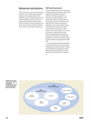
![Typical basic life and C/P values and mean wheel diameters
Basic rating life, C/P Mean wheel
Vehicle type million km value diameter DW [m]
Freight cars1) 0,8 6,84) 0,9
Mass transit vehicles
like suburban trains,
underground and
metro vehicles, light rail
and tramway vehicles
1,5 7,1÷7,7 0,7
Passenger coaches2) 33) 7,2÷8,8 0,9
Multiple units 3÷4 7,8÷9,1 1,0
Locomotives 3÷5 6,6÷8,6 1,2
1) According to UIC International Union of Railways / Union Internationale
des Chemins de fer codex, under continuously acting maximum axleload
2) According to UIC codex
3) Some operators require up to 5 million km
4) Tapered roller bearing units for AAR Association of American Railroads
applications can have, in some specific cases, a lower C/P value down to 5
Dynamic bearing loads
The loads acting on a bearing can be
calculated according to the laws of
mechanics if the external forces, e.g.
axleload, weight of the wheelset and payload
are known or can be calculated. When
calculating the load components for a single
bearing, the axle journal is considered as a
beam resting on rigid, moment–free bearing
supports. Elastic deformation in the bearing,
axlebox housing or bogie frame components
are not considered in the basic rating life
calculation. As well, resulting moments on
the bearing due to elastic deflection of shaft,
axlebox or suspension are not taken into
account. The reason is that it is not only the
shaft that creates moments.
These simplifications help to calculate the
basic rating life, using readily available
means such as a pocket calculator. The
standardized methods for calculating basic
load ratings and equivalent bearing loads
are based on similar assumptions.
G =
G00 – Gr
2
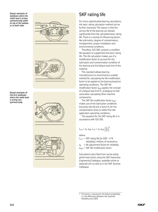
Acting bearing loads principles
Ka = axial load
G00 = static axleload
Gr = wheelset mass
Static bearing load
5
109](https://image.slidesharecdn.com/rtb-1-05-bearing-calculation-181109025220/85/Rtb-1-05-bearing-calculation-5-320.jpg)
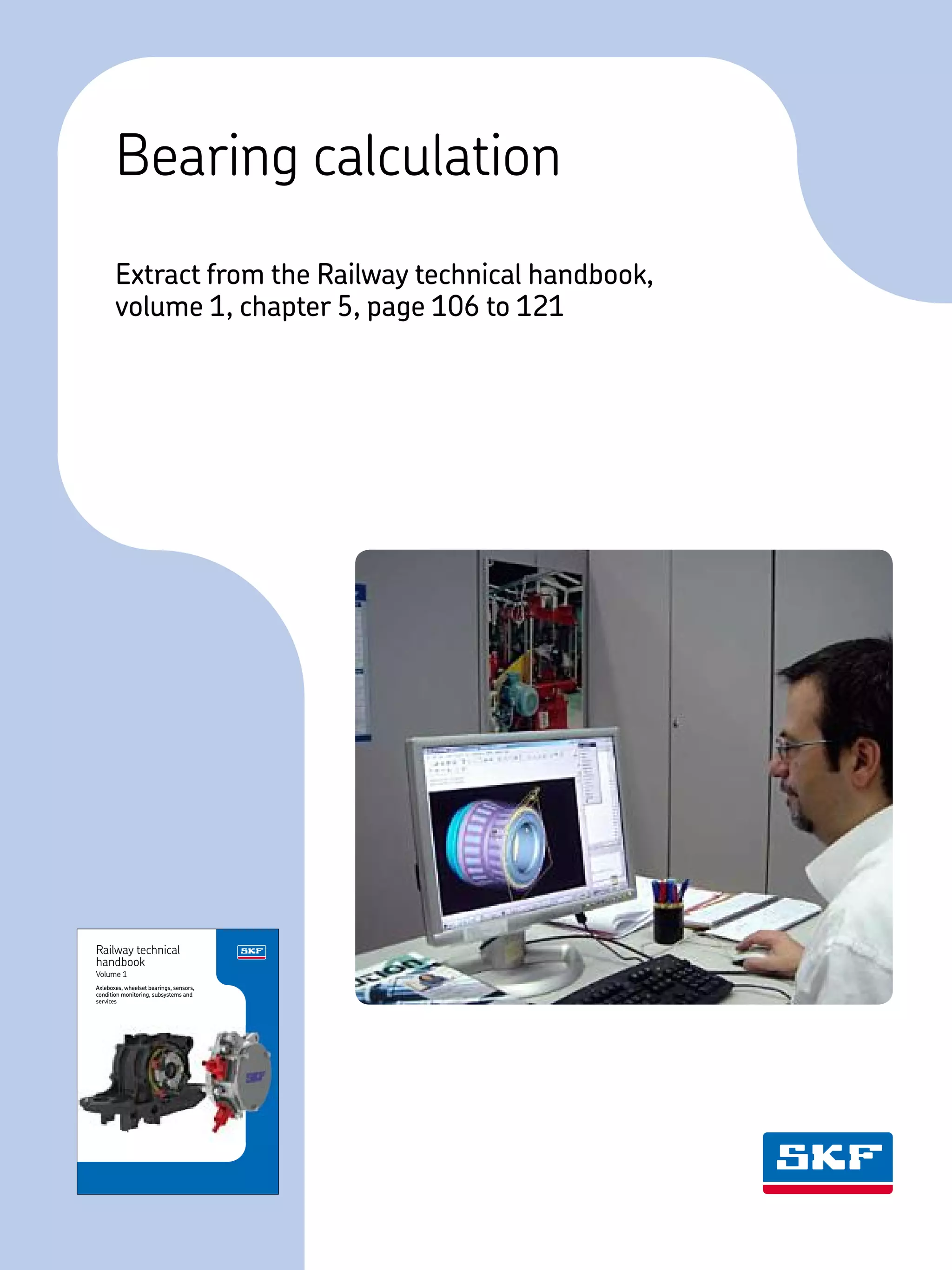
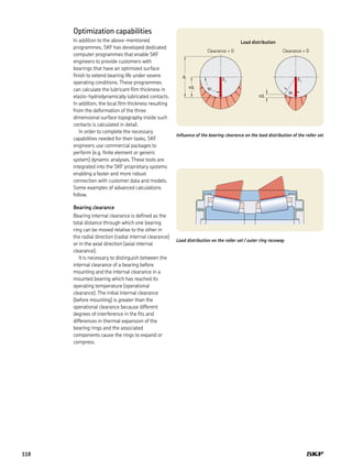
![Radial bearing load
The maximum static axlebox load per
bearing arrangement/unit is obtained from:
where
G = maximum static axlebox load [kN]
G00 = maximum static axleload [kN]
Gr = weight of the wheelset [kN]
Based on the static axlebox load, the mean
radial load is calculated by considering any
variations in the payload as well as any
additional dynamic radial forces
Kr = f0 frd ftr G
where
Kr = mean radial load [kN]
f0 = payload factor
frd = dynamic radial factor
ftr = dynamic traction factor
For standard applications, usually the mean
values are used, e.g. frd = 1,2 for passenger
coaches in standard applications.
For specific applications like high-speed
and very high-speed applications or specific
dynamic effects like irregularities of the rails,
hunting of bogies etc., the dynamic load
factor frd has to be agreed by the customer.
These additional dynamic loads are in many
cases the result of field test recordings and
statistical analysis. In principle, the
dispersion of the dynamic load increases
with the speed.
Payload factor f0 Vehicle type
0,8 to 0,9 Freight cars
0,9 to 1 Multiple units, passenger coaches and
mass transit vehicles
1 Locomotives and other vehicles having a
constant payload
The pay load factor f0 is used for variation in the static loading of the
vehicle, e.g. goods for freight and passengers incl. baggage for coaches.
A locomotive has no significant variation in the static load; that’s why
a full static axlebox load needs to be applied.
Dynamic radial factor frd Vehicle type
1,2 Freight cars, adapter application
1,1 to 1,3 Multiple units, passenger coaches and
mass transit vehicles
1,2 to 1,4 Locomotives and other vehicles having a
constant payload
The dynamic radial factor frd is used to take into account quasi-static
effects like rolling and pitch as well as dynamic effects from the wheel
rail contact.
Dynamic traction factor ftr Vehicle type
1,05 Powered vehicles with an elastic drive
system, e.g. hollow shaft drive with elastic
coupling
1,1 Powered vehicles with a non-elastic drive
system, e.g. axle hung traction motors
1 Non-powered vehicles
The dynamic traction factor is used to take into account additional radial
loads caused by the drive system.
Dynamic axial factor fad Vehicle type
0,1 Freight cars
0,08 Multiple units, passenger coaches and
mass transit vehicles, max speed
160 km/h
0,1 Multiple units, passenger coaches and
mass transit vehicles > 160 km/h
0,12 Locomotives, tilting trains or other
concepts leading to higher lateral
acceleration
110](https://image.slidesharecdn.com/rtb-1-05-bearing-calculation-181109025220/85/Rtb-1-05-bearing-calculation-6-320.jpg)
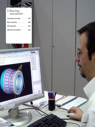
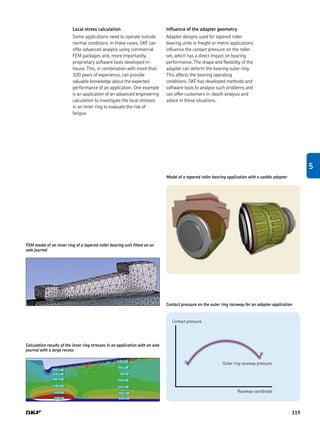
![Symmetrical axleboxes
In most cases, the radial load is acting
symmetrically either on top of the axlebox or
on both sides.
In case of such symmetrical axlebox
designs:
Fr = Kr
where
Fr = radial bearing load [kN]
Non-symmetrical axleboxes
Non-symmetrical axleboxes, like link arm
designs, have to be specially calculated as
mentioned in the calculation example 2
(† page 114).
Axial bearing load
The mean axial load is calculated by
considering the dynamic axial forces on the
axlebox.
Ka = f0 fad G
where
fad = dynamic axial factor
Fa = Ka
Equivalent bearing load P
The equivalent bearing load to be used for
the L10 basic rating life calculation either as
described before or based on specific
customer load configurations is as follows:
P = Fr + Y Fa for tapered roller bearings
and spherical roller bearings
P = Fr for cylindrical roller bearings
where
P = equivalent dynamic bearing load [kN]
Y = axial load bearing factor
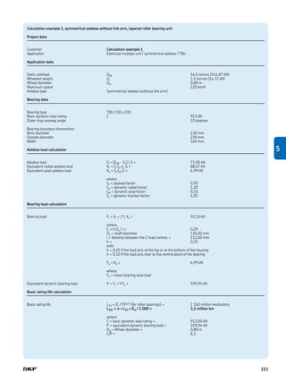
l
Link arm axlebox calculation model
lh 5
111](https://image.slidesharecdn.com/rtb-1-05-bearing-calculation-181109025220/85/Rtb-1-05-bearing-calculation-7-320.jpg)

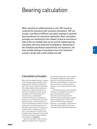
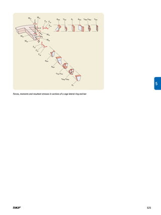
![20 000 [N]
15 000
10 000
5 000
0
90°
270° [deg]
180° 0°
90°
270°
180° 0°
14 000
10 000
6 000
2 000
0
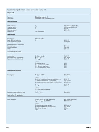
Input data example,
geometry of outer
ring, roller, flange and
raceway
SKF bearing beacon
calculated roller
contact loads
The red and blue
colours relate to the
two different roller
bearing sets. The
calculation is typically
done for various load
conditions. As an
example, two of them
feature here
X
B
A
r2 r4
b
h3e
he
Dik
Dmin
Mw
Pw
R
A
0
5
117](https://image.slidesharecdn.com/rtb-1-05-bearing-calculation-181109025220/85/Rtb-1-05-bearing-calculation-13-320.jpg)
![Cage modelling and calculation
In operation, the rolling elements pass from
the loaded into the unloaded zone where
the cage has to guide them. SKF developed
this simulation method for bearings in
railway applications to analyse the elastic
behaviour of the cage under all types of
vibrations and shocks, such as the influence
of wheel flats and rail joints. The cage is
modelled as an elastic structure where the
cage mass is uniformly distributed over each
mass centre of the cage bars (prongs) that
are connected by springs with radial,
tangential and bending stiffness. The motion
of each mass of rolling elements is described
by a group of differential equations that are
numerically solved in the simulation
programme. The results of these equations
have been verified experimentally, based on
operating conditions covering most practical
situations.
The inertia and support forces acting on
the cage produce internal stresses. In the
model of a cage cross section, the internal
forces, F, and the moments, M, acting on the
cross sections of the bars, s, and the lateral
ring, r, are displayed. The nominal value of
the normal stress is calculated as a function
of the longitudinal forces and bending
moments, while the nominal value of shear
stress is derived from the transverse forces
and the torsional moments. The stress
components can be combined into an
equivalent stress according to the form
change energy hypothesis [25].
0
a
s
as
a
bel
beA
bek
bk
Cr
Ct
Cd
bA
b1
b
e1
0L
Sk
FL
A
Sw
W
k
l
eA
ek rk
r
Dynamic model for simulation of the cage
forces
Calculation results of a FEM design optimization
of a cage lateral ring and bar of a tapered roller
bearing unit polymer cage
120](https://image.slidesharecdn.com/rtb-1-05-bearing-calculation-181109025220/85/Rtb-1-05-bearing-calculation-16-320.jpg)
![® SKF, AMPEP, @PTITUDE, AXLETRONIC, EASYRAIL, INSOCOAT, MRC, MULTILOG are registered trademarks of the SKF Group.
All other trademarks are the property of their respective owner.
© SKF Group 2012
The contents of this publication are the copyright of the publisher and may not be reproduced (even extracts) unless prior written
permission is granted. Every care has been taken to ensure the accuracy of the information contained in this publication but no liability can
be accepted for any loss or damage whether direct, indirect or consequential arising out of the use of the information contained herein.
PUB 42/P2 12789 EN · 2012
Certain image(s) used under license from Shutterstock.com
Bearings
and units
Seals
Lubrication
systems
Mechatronics Services
The Power of Knowledge Engineering
Drawing on five areas of competence and application-specific expertise amassed over more than 100
years, SKF brings innovative solutions to OEMs and production facilities in every major industry world-
wide. These five competence areas include bearings and units, seals, lubrication systems, mechatronics
(combining mechanics and electronics into intelligent systems), and a wide range of services, from 3-D
computer modelling to advanced condition monitoring and reliability and asset management systems.
A global presence provides SKF customers uniform quality standards and worldwide product availability.
References
Liang, B.:[25] Berechnungsgleichungen für Reibmomente in Planetenwälzlagern. Ruhr-
Universität Bochum. Fakultät für Maschinenbau, Institut für Konstruktionstechnik.
Schriftenreihe Heft 92.3.
www.railways.skf.com](https://image.slidesharecdn.com/rtb-1-05-bearing-calculation-181109025220/85/Rtb-1-05-bearing-calculation-18-320.jpg)

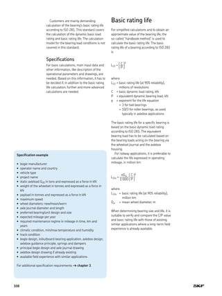
This document provides guidance on calculating bearing life for railway applications. It discusses calculation principles, basic rating life calculations according to ISO 281, and more advanced SKF rating life calculations. It also provides example calculations for typical symmetrical and link arm axlebox designs, showing how to determine static and dynamic bearing loads based on vehicle specifications in order to calculate the basic or SKF rating life in millions of revolutions or kilometers.