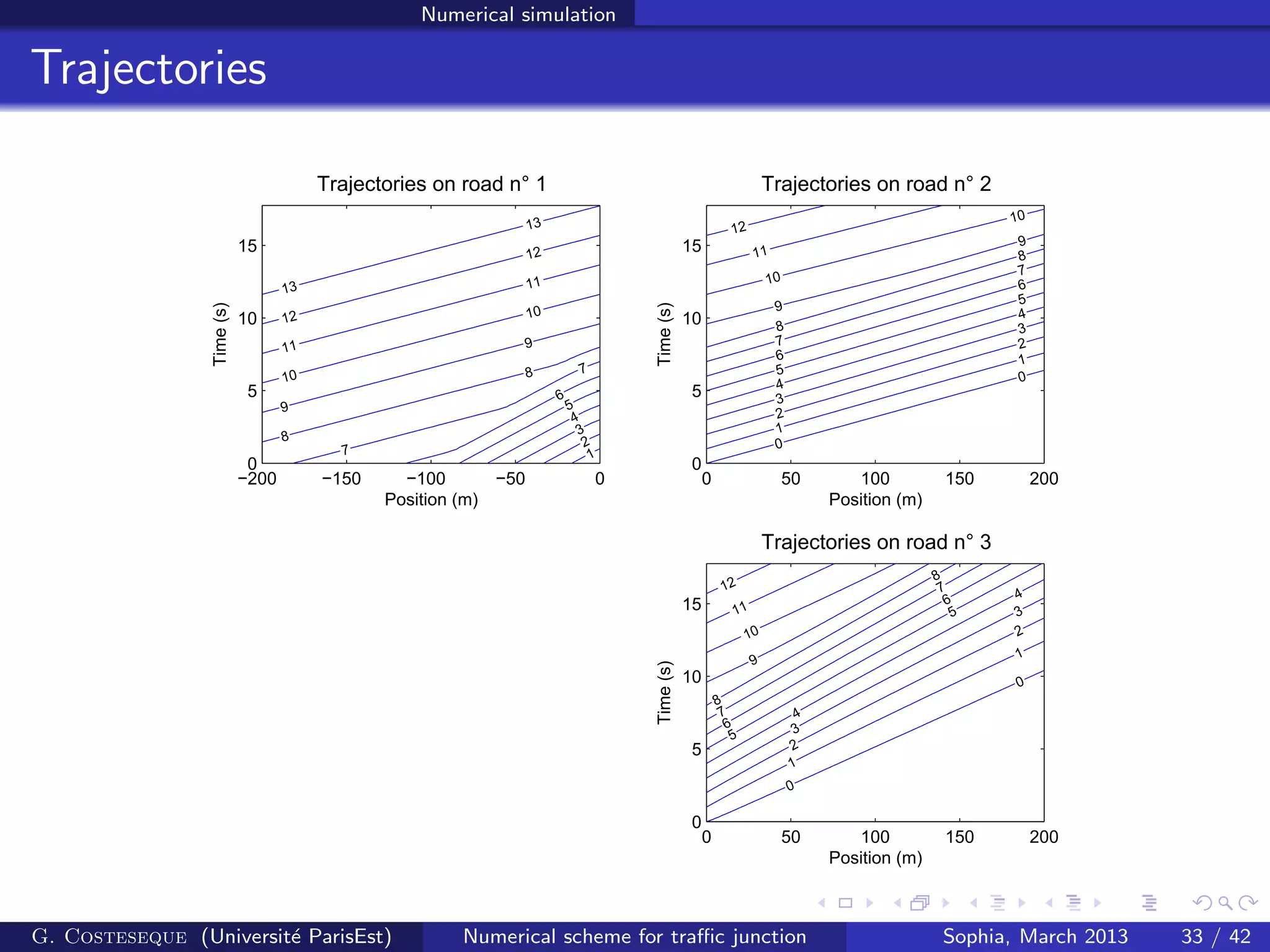
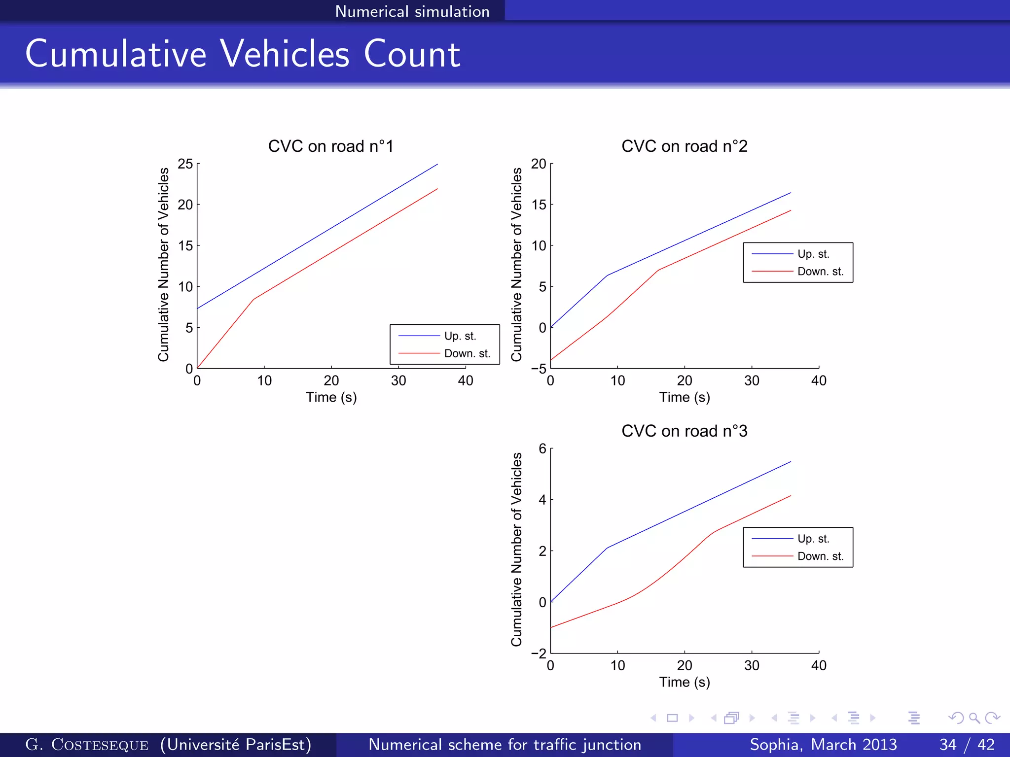
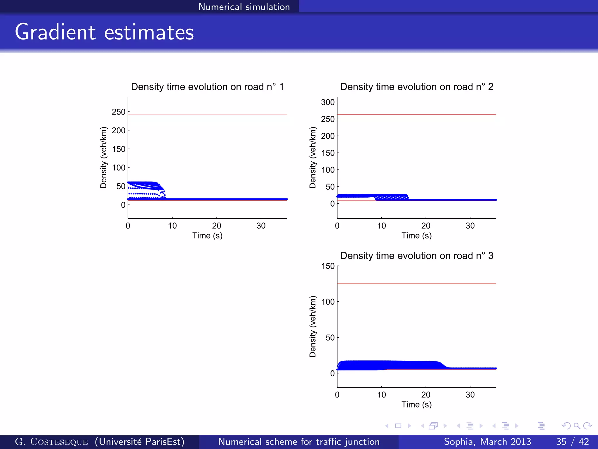
The document summarizes a numerical scheme for modeling traffic flow at road junctions using Hamilton-Jacobi equations. The scheme models traffic on each branch of the junction as well as at the junction point where branches meet. It introduces Hamiltonians representing traffic flow and establishes gradient estimates and existence/uniqueness results for the numerical solution. The scheme is shown to converge to the unique viscosity solution of the underlying partial differential equations as the grid is refined.


![Motivation
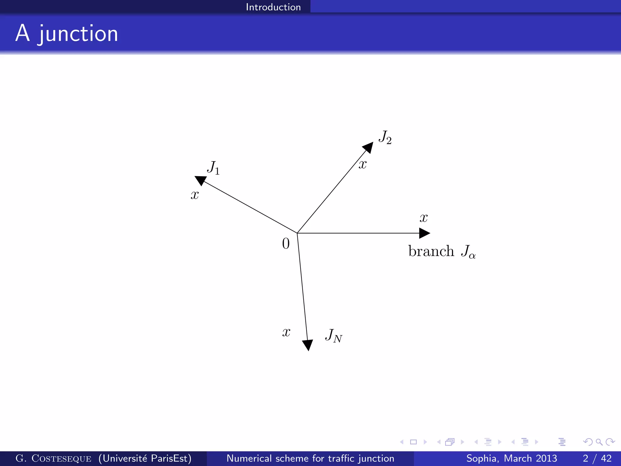
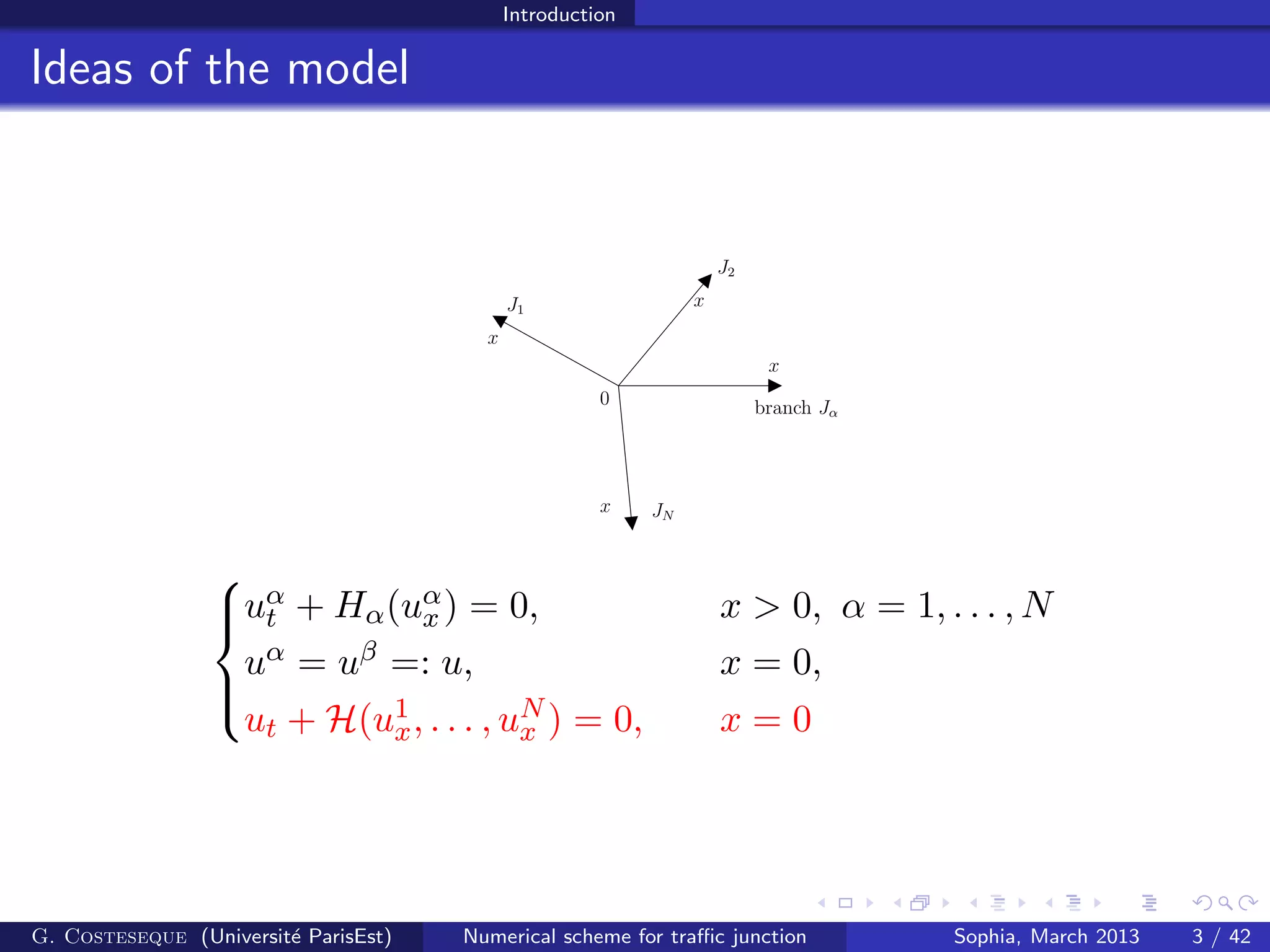
The simple divergent road
x > 0
x > 0γl
γrx < 0
Il
Ir
γe
Ie
γe = 1,
0 ≤ γl, γr ≤ 1,
γl + γr = 1
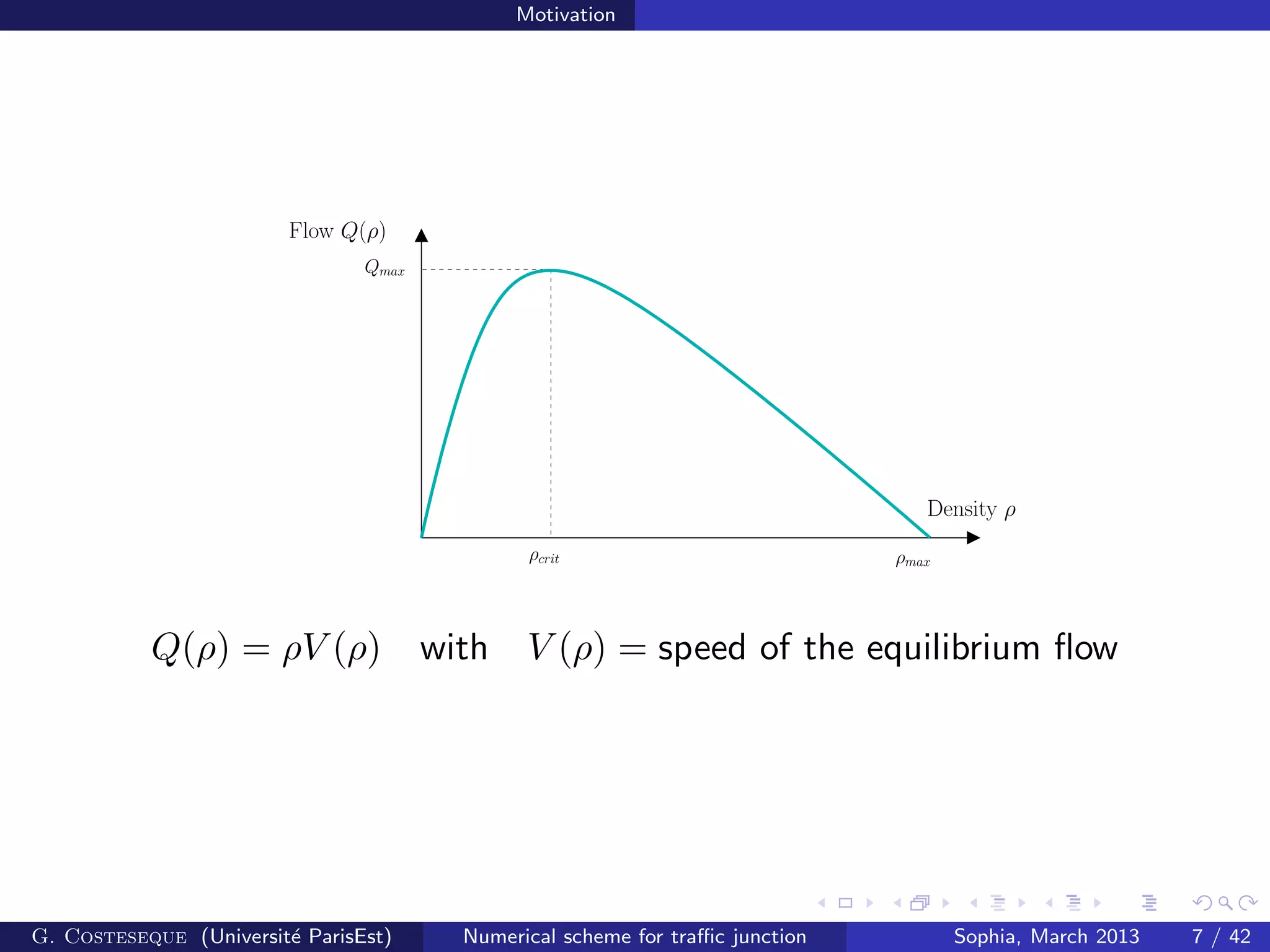
LWR model [Lighthill, Whitham ’55; Richards ’56]:
ρt + (Q(ρ))x = 0
G. Costeseque (Universit´e ParisEst) Numerical scheme for traffic junction Sophia, March 2013 6 / 42](https://image.slidesharecdn.com/workshopsophia-costeseque-v3-190806053521/75/Road-junction-modeling-using-a-scheme-based-on-Hamilton-Jacobi-equations-6-2048.jpg)

![Junction model and adapted scheme Mathematical results
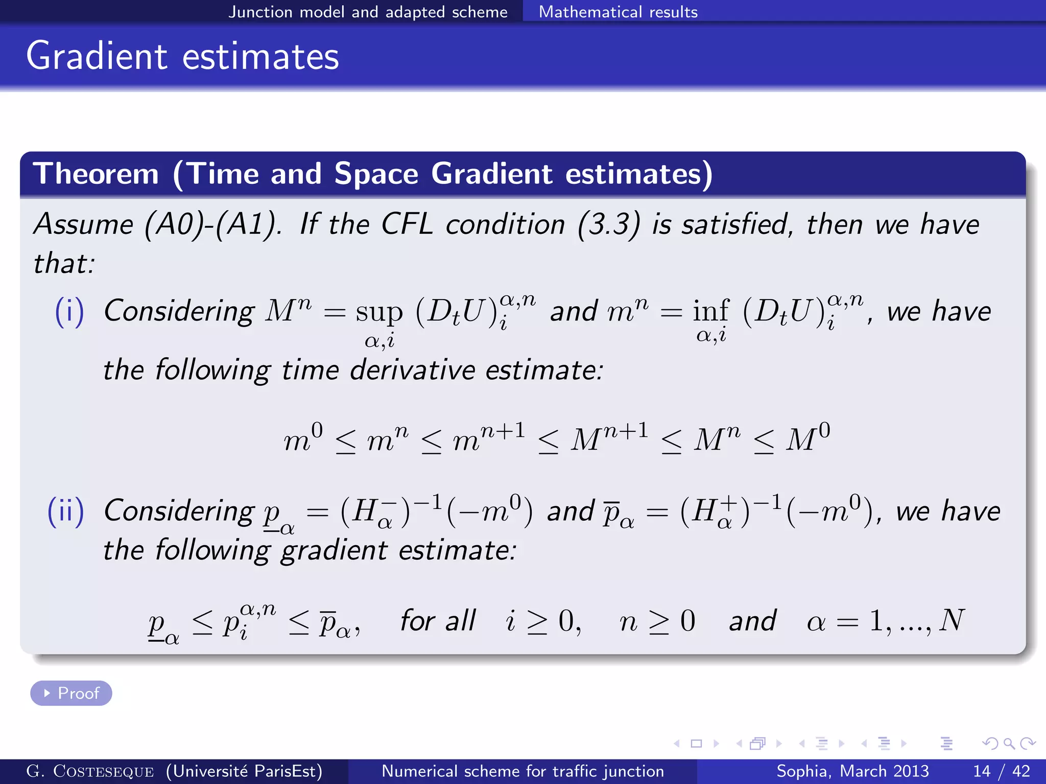
Stronger CFL condition
As for any α = 1, . . . , N, we have that:
pα
≤ pα,n
i ≤ pα for all i, n ≥ 0
−m0
pα
p
Hα(p)
pα
Then the CFL condition becomes:
∆x
∆t
≥ sup
α=1,...,N
pα∈[pα
,pα]
|H′
α(pα)| (3.4)
G. Costeseque (Universit´e ParisEst) Numerical scheme for traffic junction Sophia, March 2013 15 / 42](https://image.slidesharecdn.com/workshopsophia-costeseque-v3-190806053521/75/Road-junction-modeling-using-a-scheme-based-on-Hamilton-Jacobi-equations-16-2048.jpg)
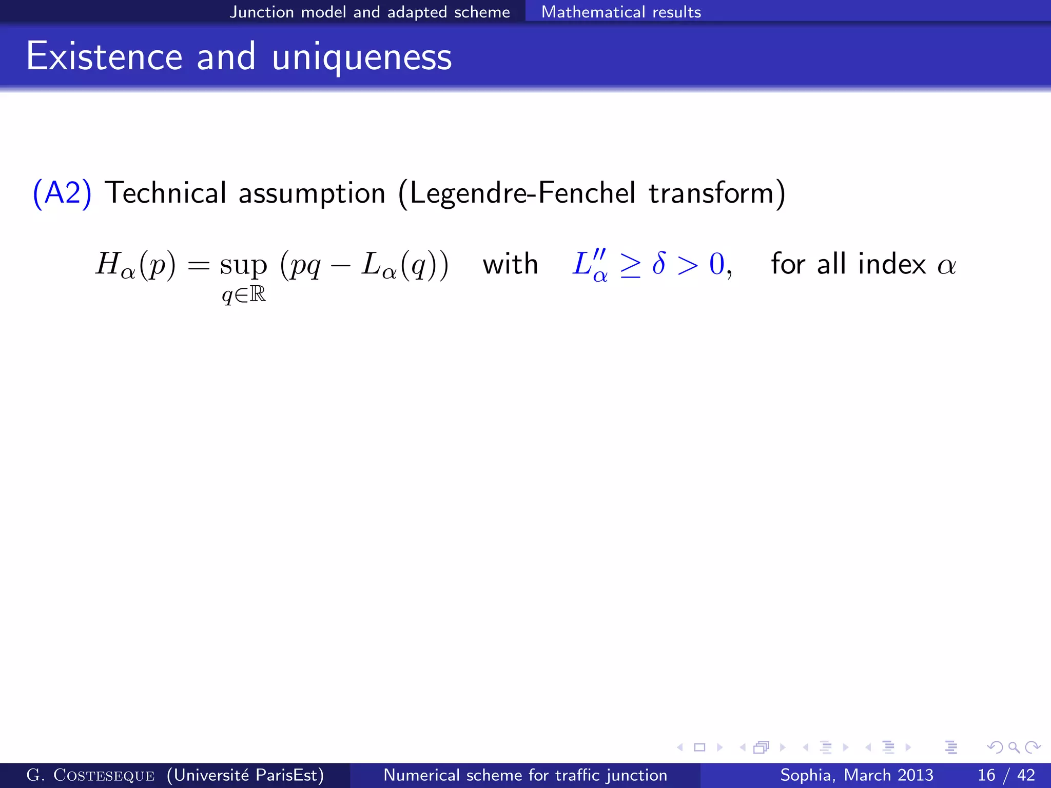
![Junction model and adapted scheme Mathematical results
Existence and uniqueness
(A2) Technical assumption (Legendre-Fenchel transform)
Hα(p) = sup
q∈R
(pq − Lα(q)) with L′′
α ≥ δ > 0, for all index α
Theorem (Existence and uniqueness [IMZ, ’11])
Under (A0)-(A1)-(A2), there exists a unique viscosity solution u of (3.1)
on the junction, satisfying for some constant CT > 0
|u(t, y) − u0(y)| ≤ CT for all (t, y) ∈ JT .
Moreover the function u is Lipschitz continuous with respect to (t, y).
G. Costeseque (Universit´e ParisEst) Numerical scheme for traffic junction Sophia, March 2013 16 / 42](https://image.slidesharecdn.com/workshopsophia-costeseque-v3-190806053521/75/Road-junction-modeling-using-a-scheme-based-on-Hamilton-Jacobi-equations-18-2048.jpg)
![Junction model and adapted scheme Mathematical results
Convergence
Theorem (Convergence from discrete to continuous [CML, ’13])
Assume that (A0)-(A1)-(A2) and the CFL condition (3.4) are satisfied.
Then the numerical solution converges uniformly to u the unique viscosity
solution of (3.1) when ε → 0, locally uniformly on any compact set K:
lim sup
ε→0
sup
(n∆t,i∆x)∈K
|uα
(n∆t, i∆x) − Uα,n
i | = 0
Proof
G. Costeseque (Universit´e ParisEst) Numerical scheme for traffic junction Sophia, March 2013 17 / 42](https://image.slidesharecdn.com/workshopsophia-costeseque-v3-190806053521/75/Road-junction-modeling-using-a-scheme-based-on-Hamilton-Jacobi-equations-19-2048.jpg)
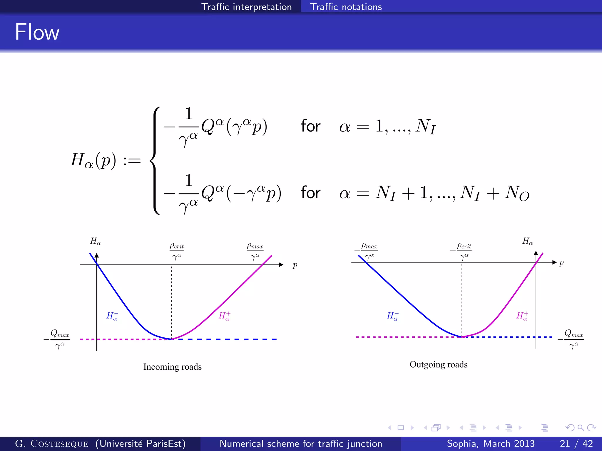
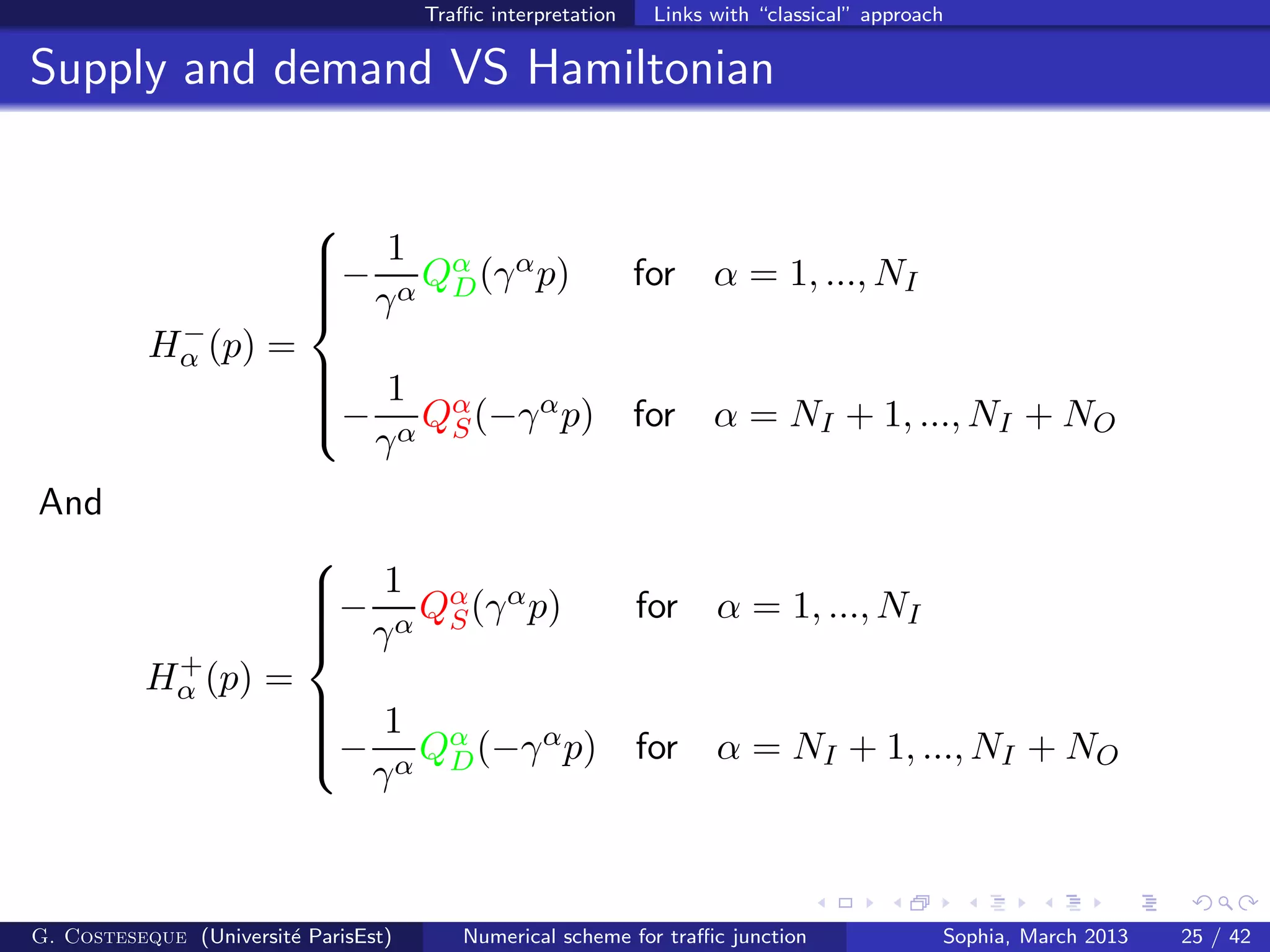
![Traffic interpretation Links with “classical” approach
Supply and demand functions
Remark
It recovers the seminal Godunov scheme with passing flow = minimum
between upstream demand QD and downstream supply QS.
Density ρ
ρcrit ρmax
Supply QS
Qmax
Density ρ
ρcrit ρmax
Flow Q
Qmax
Density ρ
ρcrit
Demand QD
Qmax
From [Lebacque ’93, ’96]
G. Costeseque (Universit´e ParisEst) Numerical scheme for traffic junction Sophia, March 2013 24 / 42](https://image.slidesharecdn.com/workshopsophia-costeseque-v3-190806053521/75/Road-junction-modeling-using-a-scheme-based-on-Hamilton-Jacobi-equations-26-2048.jpg)
![Traffic interpretation Literature review
Some references for conservation laws
ρt + (Q(x, ρ))x = 0 with Q(x, p) = 1{x<0}Qin
(p) + 1{x≥0}Qout
(p)
Uniqueness results only for restricted configurations:
See [Garavello, Natalini, Piccoli, Terracina ’07]
and [Andreianov, Karlsen, Risebro ’11]
Book of [Garavello, Piccoli ’06] for conservation laws on networks:
Construction of a solution using the “wave front tracking method”
No proof of the uniqueness of the solution on a general network
G. Costeseque (Universit´e ParisEst) Numerical scheme for traffic junction Sophia, March 2013 26 / 42](https://image.slidesharecdn.com/workshopsophia-costeseque-v3-190806053521/75/Road-junction-modeling-using-a-scheme-based-on-Hamilton-Jacobi-equations-28-2048.jpg)
![Traffic interpretation Literature review
Numerics on networks
Godunov scheme mainly used for conservation laws:
[Bretti, Natalini, Piccoli ’06, ’07]: Godunov scheme compared to
kinetic schemes / fast algorithms
[Blandin, Bretti, Cutolo, Piccoli ’09]: Godunov scheme adapted for
Colombo model (only tested for 1 × 1 junctions)
G. Costeseque (Universit´e ParisEst) Numerical scheme for traffic junction Sophia, March 2013 27 / 42](https://image.slidesharecdn.com/workshopsophia-costeseque-v3-190806053521/75/Road-junction-modeling-using-a-scheme-based-on-Hamilton-Jacobi-equations-29-2048.jpg)
![Traffic interpretation Literature review
Numerics on networks
Godunov scheme mainly used for conservation laws:
[Bretti, Natalini, Piccoli ’06, ’07]: Godunov scheme compared to
kinetic schemes / fast algorithms
[Blandin, Bretti, Cutolo, Piccoli ’09]: Godunov scheme adapted for
Colombo model (only tested for 1 × 1 junctions)
[Han, Piccoli, Friesz, Yao ’12]: Lax-Hopf formula for HJ equation coupled
with a Riemann solver at junction
G. Costeseque (Universit´e ParisEst) Numerical scheme for traffic junction Sophia, March 2013 27 / 42](https://image.slidesharecdn.com/workshopsophia-costeseque-v3-190806053521/75/Road-junction-modeling-using-a-scheme-based-on-Hamilton-Jacobi-equations-30-2048.jpg)
![Traffic interpretation Literature review
Junction modelling
State-of-the-art review:
[Lebacque, Khoshyaran ’02, ’05, ’09]
[Tamp`ere, Corthout, Cattrysse, Immers ’11],
[Fl¨otter¨od, Rohde ’11]
Calibration of γα for realistic models:
[Cassidy and Ahn ’05]
[Bar-Gera and Ahn ’10],
[Ni and Leonard ’05] (small data set)
G. Costeseque (Universit´e ParisEst) Numerical scheme for traffic junction Sophia, March 2013 28 / 42](https://image.slidesharecdn.com/workshopsophia-costeseque-v3-190806053521/75/Road-junction-modeling-using-a-scheme-based-on-Hamilton-Jacobi-equations-31-2048.jpg)
![Conclusion
Complementary results [CML ’13]:
Generalization for weaker assumptions on the Hamiltonians
Numerical simulation for other junction configurations (merge)
G. Costeseque (Universit´e ParisEst) Numerical scheme for traffic junction Sophia, March 2013 37 / 42](https://image.slidesharecdn.com/workshopsophia-costeseque-v3-190806053521/75/Road-junction-modeling-using-a-scheme-based-on-Hamilton-Jacobi-equations-40-2048.jpg)
![Conclusion
Complementary results [CML ’13]:
Generalization for weaker assumptions on the Hamiltonians
Numerical simulation for other junction configurations (merge)
Open questions:
Error estimate
Non-fixed coefficients γα
Other link models (GSOM)
Other junction condition
G. Costeseque (Universit´e ParisEst) Numerical scheme for traffic junction Sophia, March 2013 37 / 42](https://image.slidesharecdn.com/workshopsophia-costeseque-v3-190806053521/75/Road-junction-modeling-using-a-scheme-based-on-Hamilton-Jacobi-equations-41-2048.jpg)
![Proofs of the main results
Sketch of the proof (gradient estimates):
Time derivative estimate:
1. Estimate on mα,n = inf
i
(DtU)α,n
i and partial result for mn = inf
α
mα,n
2. Similar estimate for Mn
3. Conclusion
Space derivative estimate:
1. New bounded Hamiltonian ˜Hα(p) for p ≤ pα
and p ≥ pα
2. Time derivative estimate from above
3. Lemma: if for any (i, n, α), (DtU)α,n
i ≥ m0 then
pα
≤ pα,n
i ≤ pα
4. Conclusion as ˜Hα = Hα on [pα
, pα]
Back
G. Costeseque (Universit´e ParisEst) Numerical scheme for traffic junction Sophia, March 2013 40 / 42](https://image.slidesharecdn.com/workshopsophia-costeseque-v3-190806053521/75/Road-junction-modeling-using-a-scheme-based-on-Hamilton-Jacobi-equations-44-2048.jpg)