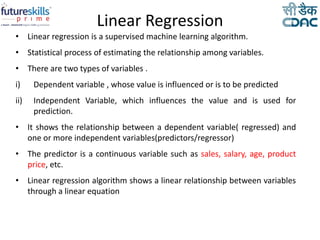
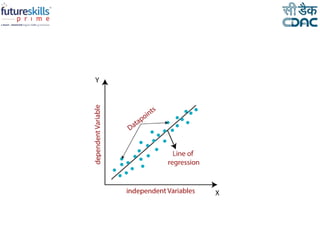
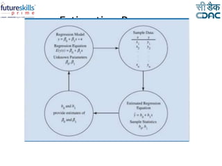
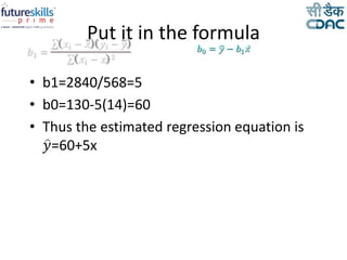
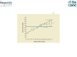
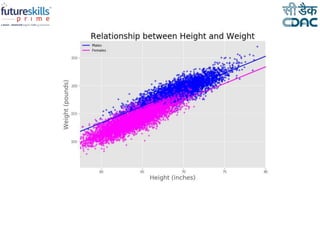
Linear regression is a machine learning technique used to model relationships between variables. It can be used to predict the value of a dependent variable based on the value of one or more independent variables. Simple linear regression uses one independent variable to predict the dependent variable, while multiple linear regression uses two or more independent variables. The linear regression equation is estimated using the least squares method to minimize error. Linear regression has various applications including predictive analytics and assessing risk.

1. Linear Regression
By: Ms. Sidhidatri Nayak
CDAC NOIDA, India

2. Objectives
• What is Regression?
• Regression Analysis
• Applications of Regression
• Simple linear regression through Least Squares Method
• Coefficient of Determination
• Using the Estimated Regression Equation for Estimation and
Prediction
• Multiple Linear Regression
• Implementation in Python

3. Linear Regression
• Linear regression is a supervised machine learning algorithm.
• Statistical process of estimating the relationship among variables.
• There are two types of variables .
i) Dependent variable , whose value is influenced or is to be predicted
ii) Independent Variable, which influences the value and is used for
prediction.
• It shows the relationship between a dependent variable( regressed) and
one or more independent variables(predictors/regressor)
• The predictor is a continuous variable such as sales, salary, age, product
price, etc.
• Linear regression algorithm shows a linear relationship between variables
through a linear equation

4. Example
• House 1 : x1: 1200sqft y1=200000
• House 2 : x2: 1500sqft y2=300000
• House 3 : x3: 1800sqft y3=400000
• House 4 : x4: 2000sqft y4=500000
• House 5: x5: 2200sqft y5=600000
• Input( x1,x2,x3,x4,x5)
• Output(y1,y2,y3,y4,y5)
• The value of y can be predicted from x, the predictor
variable.
• Y variable is the quantity of interest.

7. Regression Lines

8. Applications of Regression
• Predictive Analytics
• Example:
1. Evaluating trend and sales estimate
2. Analyzing the impact of price changes
3. Assessment of risk in financial services and
insurance domain

9. Regression Analysis
• Regression Analysis is the process of
developing a statistical model , to predict the
value of dependent variable by at least one
independent variable.

10. The Simple Linear Regression Model
• Simple Linear Regression Model
y = 0 + 1x + 
• Simple Linear Regression Equation
E(y) = 0 + 1x

11. Example
• ABC café chain located in different cities of India.
It is more popular near the university campus.
The manager believes that the quarterly sales for
the café ( denoted by y) are related to the size of
the student population (denoted by x).
• That is cafes that is near to university campus
with large student population may generate more
sales compared to others.
• Using regression analysis we can develop an
equation showing how the dependent variable y
is related to the independent variable x.

12. Estimation Process

13. Scatter plot

14. The Least Squares Method
• Slope for the Estimated Regression Equation
• Intercept for the Estimated Regression Equation
𝑏0 = 𝑦 − 𝑏1𝑥
where:
xi = value of independent variable for ith
observation
yi = value of dependent variable for ith
observation
x = mean value for independent variable
_
_
𝑏1 =
𝑥𝑖 − 𝑥 𝑦𝑖 − 𝑦
𝑥𝑖 − 𝑥 2

15. Table 2 calculating the least squares
estimated regression equation for ABC
cafe

16. Put it in the formula
• b1=2840/568=5
• b0=130-5(14)=60
• Thus the estimated regression equation is
𝑦=60+5x
𝑏0 = 𝑦 − 𝑏1𝑥

18. Table 3 for SSE

19. Table for SST

21. Finding SSR and r2
• SSR=SST-SSE=15730-1530=14200
• Coefficient of Determination
r2 = SSR/SST = 14200/15730 = .9027

24. Mean Square Error
• An Estimate of s 2
The mean square error (MSE) provides the estimate
of s 2, and the notation s2 is also used.
s2 = MSE = SSE/(n-2)

26. • MSE=SSE/(n-2)
• MSE=1530/8=191.25
• S=13.829
• The predictive precision of the linear
regression model using evaluation metrics
such as the mean square error.

27. The Multiple Regression Model
• The Multiple Regression Model
y = 0 + 1x1 + 2x2 + . . . + pxp + 
• The Multiple Regression Equation
E(y) = 0 + 1x1 + 2x2 + . . . + pxp
• The Estimated Multiple Regression
Equation
y = b0 + b1x1 + b2x2 + . . . + bpxp
^