Downloaded 38 times
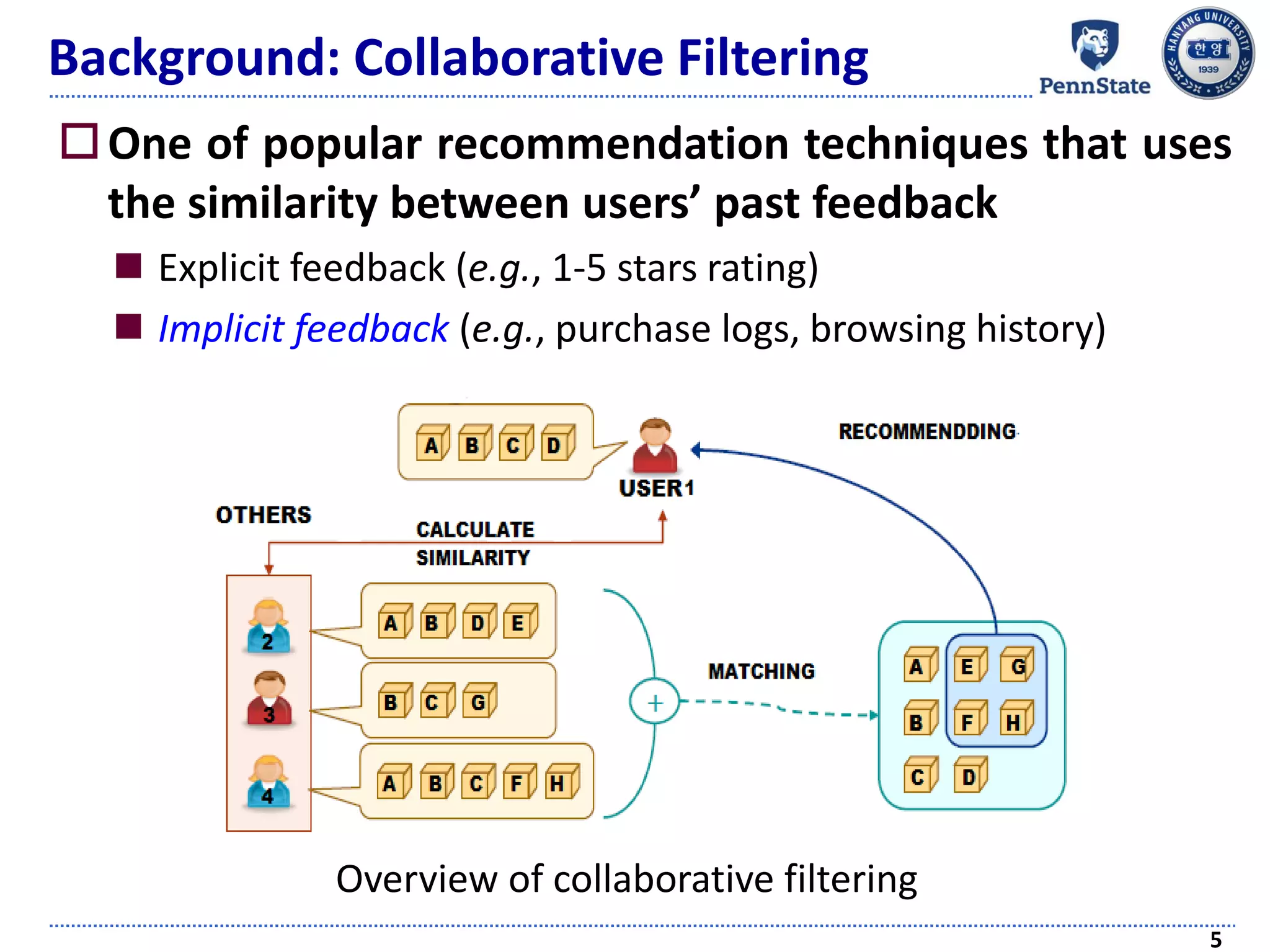
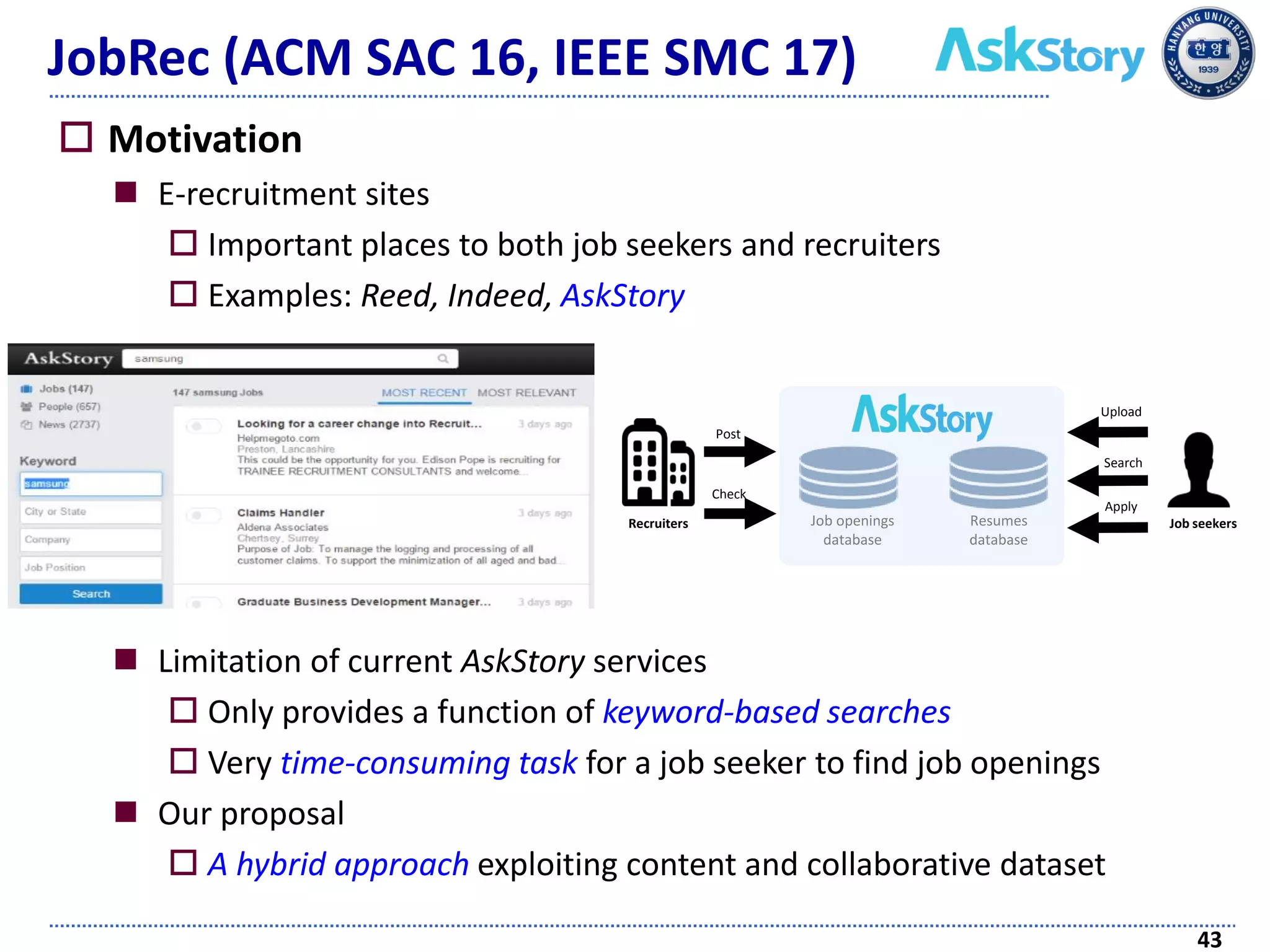
![Motivation
Zero-injection [Hwang et al., ICDE 16]
Address the sparsity problem successfully in multi-class
setting
Define a novel notion of ‘uninteresting items’ (U-items, in
short) of a user
Items on which the user has “negative” preferences
8
Whole items (𝐼u)
Interesting items
(𝐼 𝑢
𝑖𝑛
)
Uninteresting items
(𝐼 𝑢
𝑢𝑛
= 𝐼 − 𝐼 𝑢
𝑖𝑛
)
Evaluated items
(𝐼 𝑢
𝑒𝑣𝑎𝑙
)
Preferred Items
(𝐼 𝑢
𝑝𝑟𝑒
)
Venn diagram for preferences of items](https://image.slidesharecdn.com/recommendersystemswithimplicitfeedbackchallengestechniquesandapplications-180410005822/75/Recommender-Systems-with-Implicit-Feedback-Challenges-Techniques-and-Applications-8-2048.jpg)
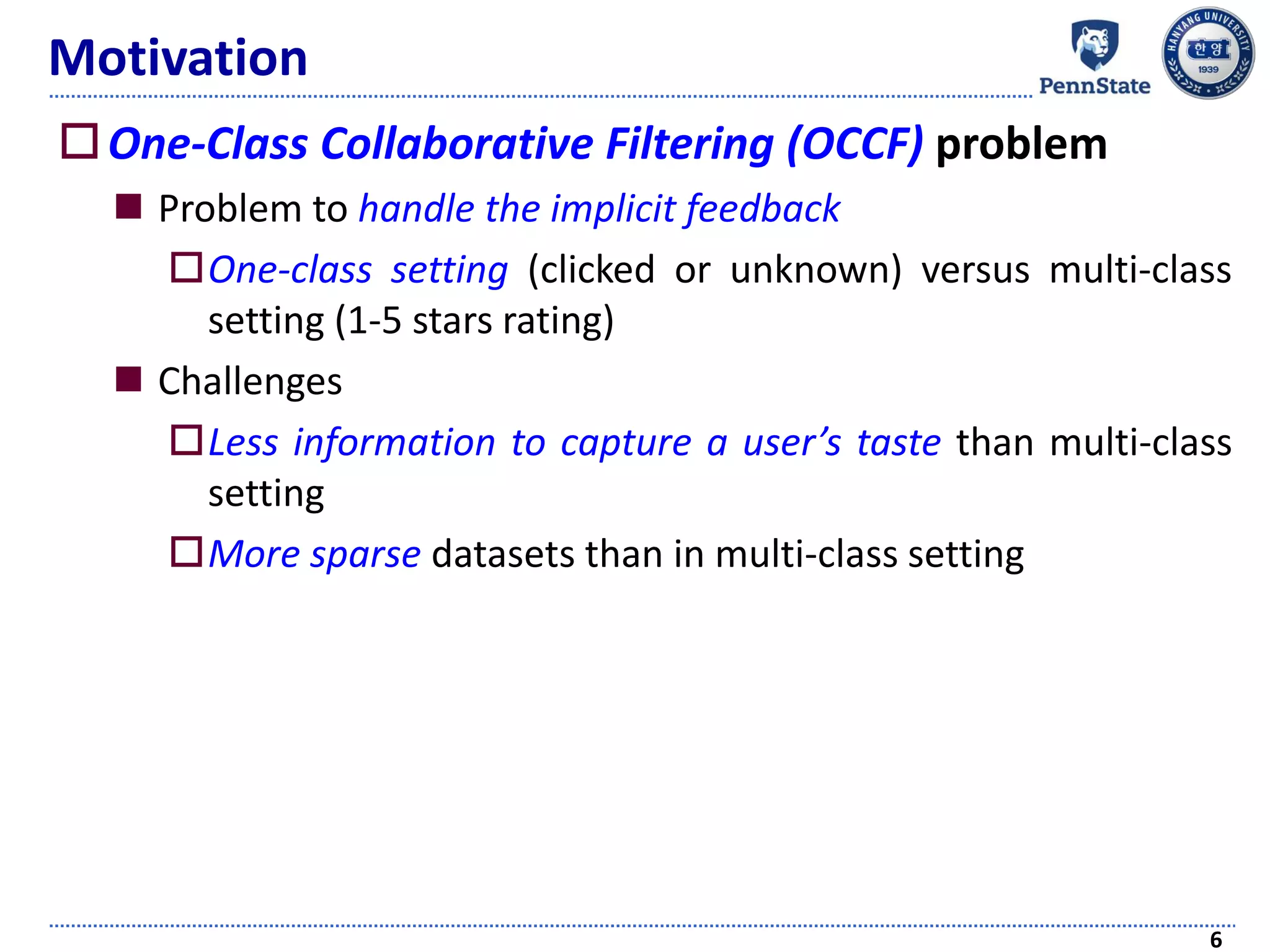
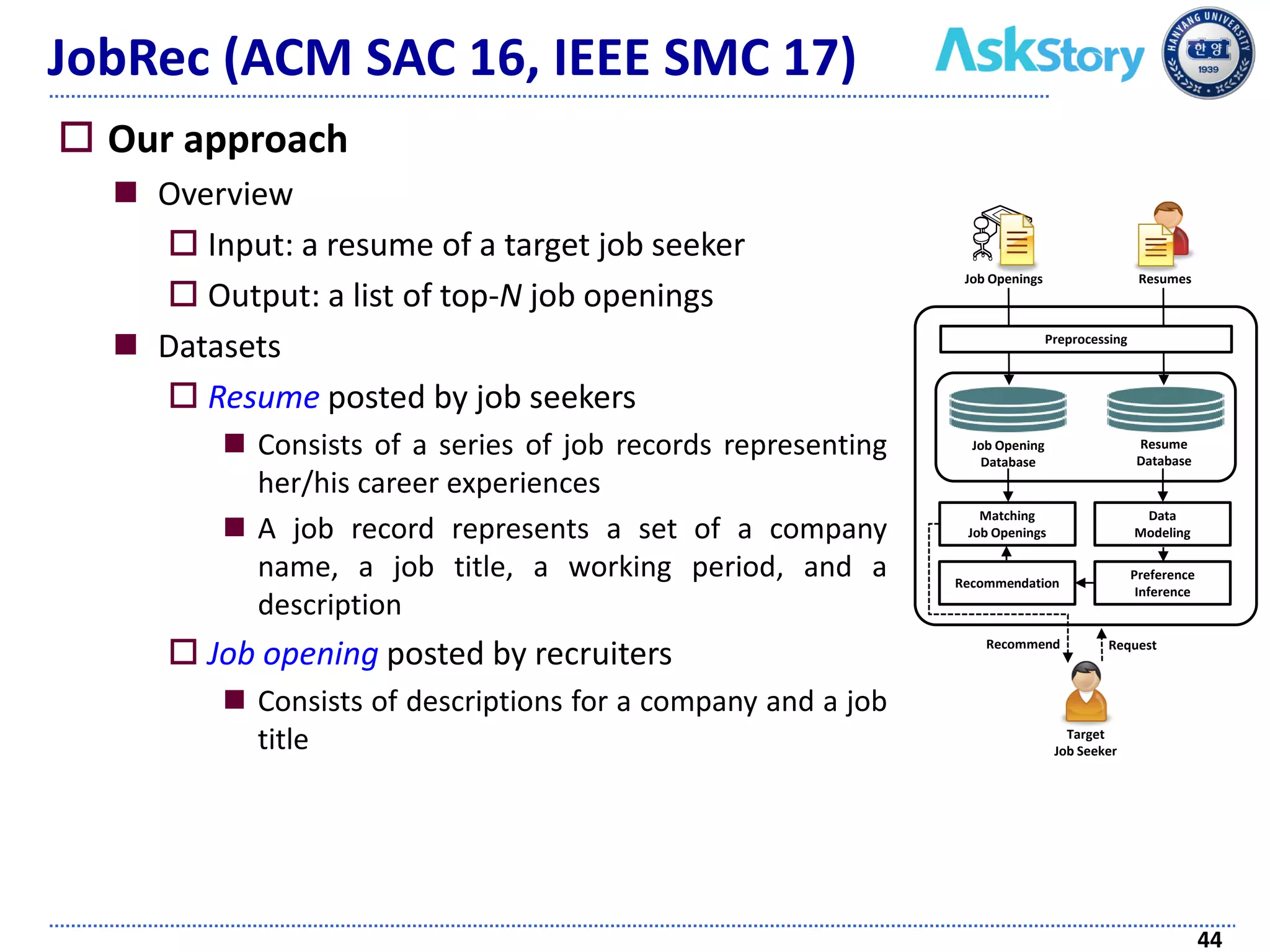
![Motivation
Zero-injection [Hwang et al., ICDE 16]
9
Overview of zero-injection](https://image.slidesharecdn.com/recommendersystemswithimplicitfeedbackchallengestechniquesandapplications-180410005822/75/Recommender-Systems-with-Implicit-Feedback-Challenges-Techniques-and-Applications-9-2048.jpg)
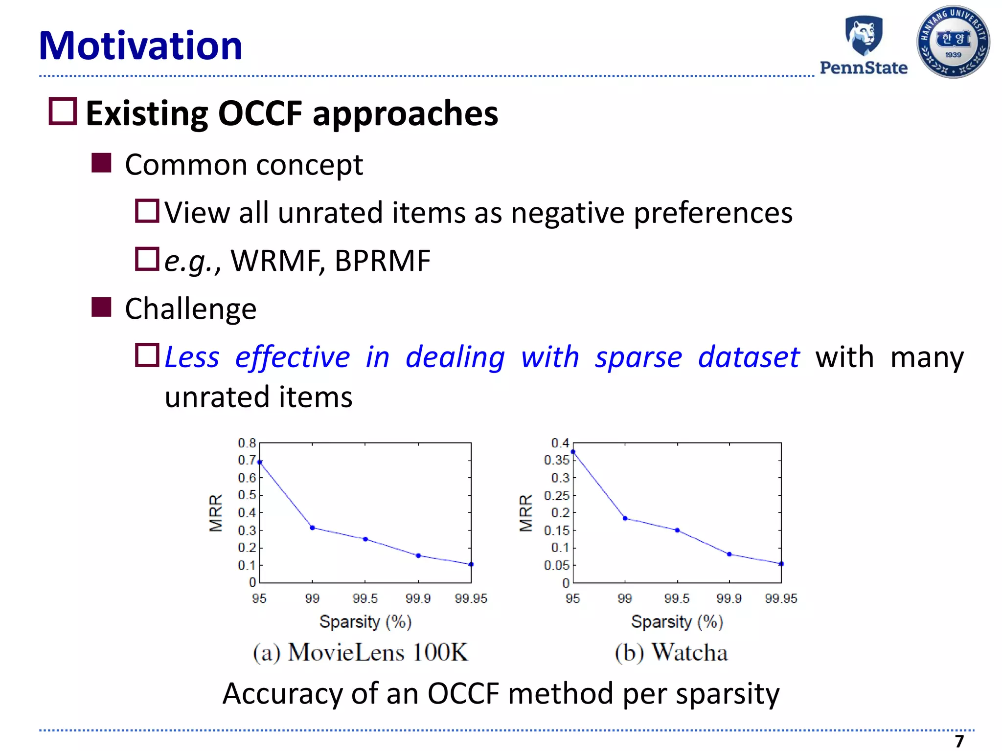
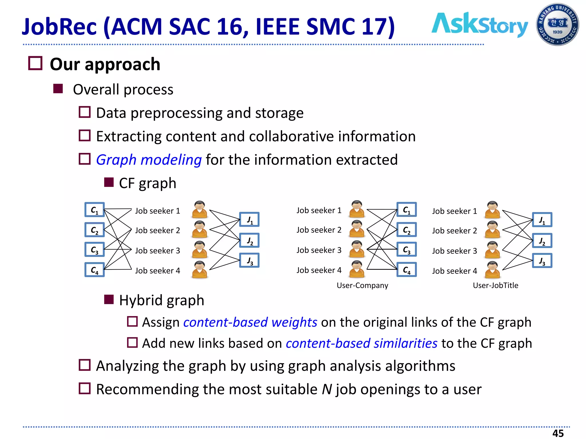
![Motivation
Zero-injection [Hwang et al., ICDE 16]
10
Accuracy of zero-injection
90 92 94 96 98 99.7
0
0.05
0.1
0.15
0.2
0.25
0 2 4 6 8 10
0
0.05
0.1
0.15
0.2
0.25
0 20 40 60 80 99.7
Precision
Parameter θ
Zero-injection + SVD
Zero-injection + ICF
<Recall>
<nDCG>
<MRR><Precision>](https://image.slidesharecdn.com/recommendersystemswithimplicitfeedbackchallengestechniquesandapplications-180410005822/75/Recommender-Systems-with-Implicit-Feedback-Challenges-Techniques-and-Applications-10-2048.jpg)
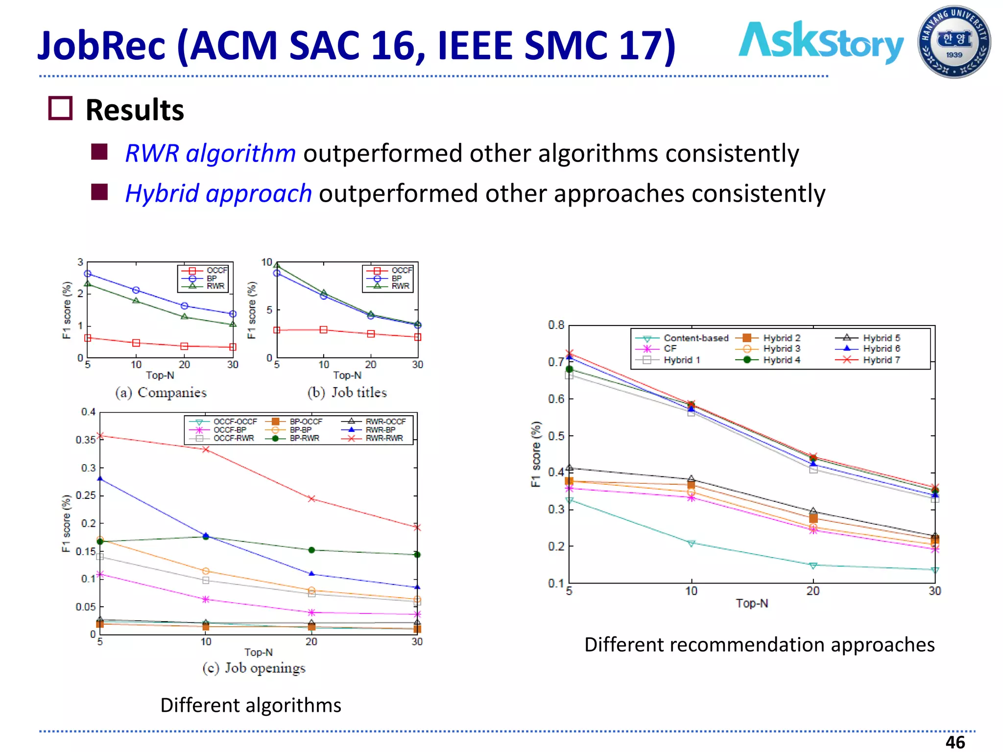
![Motivation
Zero-injection [Hwang et al., ICDE 16]
A naïve application of zero-injection in one-class setting
Lower accuracy than OCCF approaches
Sensitivity to the number of U-items
11
Accuracy in one-class setting: SVD and PMF with varying
degree of zero injection and WRMF without zero-injection](https://image.slidesharecdn.com/recommendersystemswithimplicitfeedbackchallengestechniquesandapplications-180410005822/75/Recommender-Systems-with-Implicit-Feedback-Challenges-Techniques-and-Applications-11-2048.jpg)
![Employ a popular OCCF method (WRMF) [Pan et al.,
ICDM 08]
Steps
Treat all unrated items as negative preferences (i.e., value of 0)
Assign different weights to quantify the relative contribution
Predict the value of by matrix factorization
13
U
V
Feature of user u
Feature of item i
1 1 1 0
1 0 0 0
0 0 1 0
1 1 1 0.6
1 0.2 0.2 0.2
0.2 0.2 1 0.2
Binary rating matrixUnary rating matrix
Weight matrix
1 1 1
1
1
WRMF
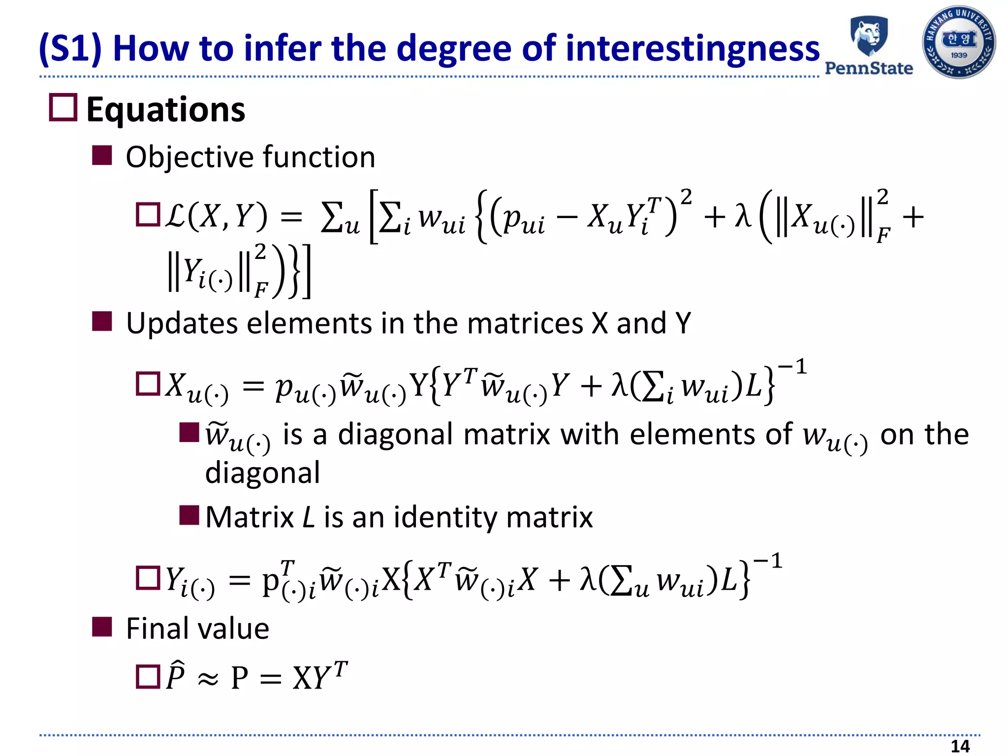
(S1) How to infer the degree of interestingness](https://image.slidesharecdn.com/recommendersystemswithimplicitfeedbackchallengestechniquesandapplications-180410005822/75/Recommender-Systems-with-Implicit-Feedback-Challenges-Techniques-and-Applications-13-2048.jpg)
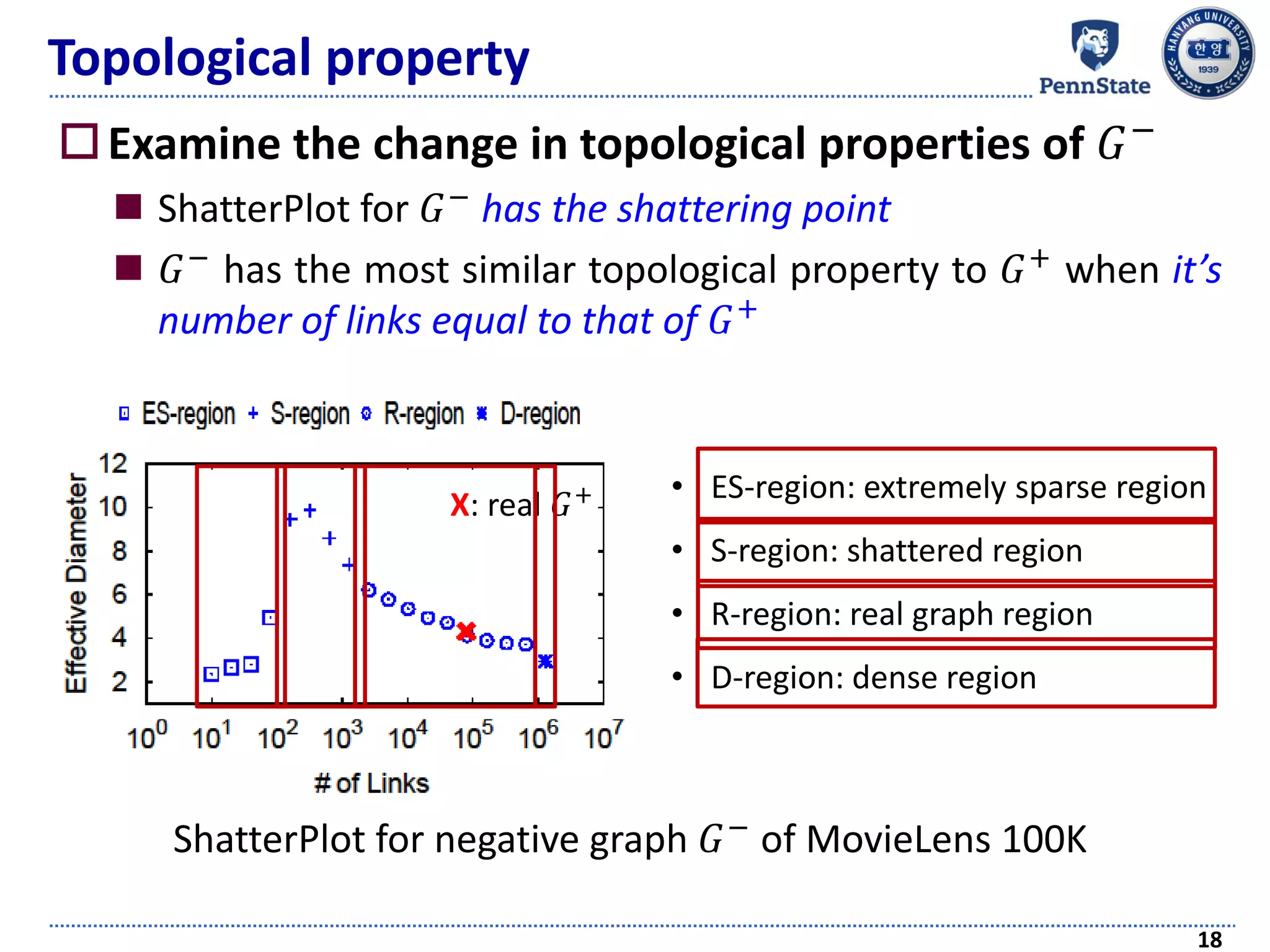
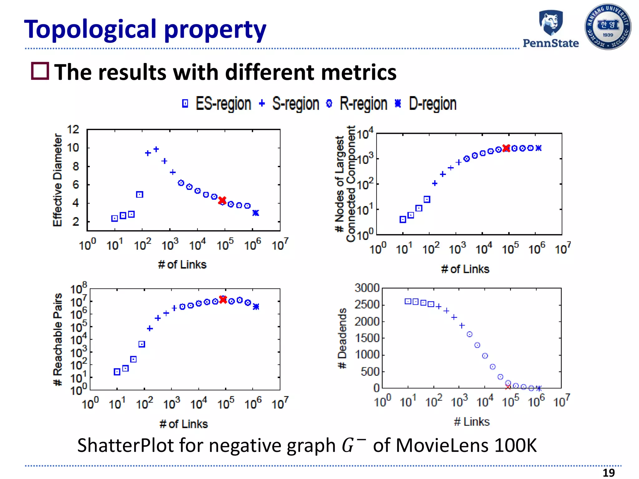
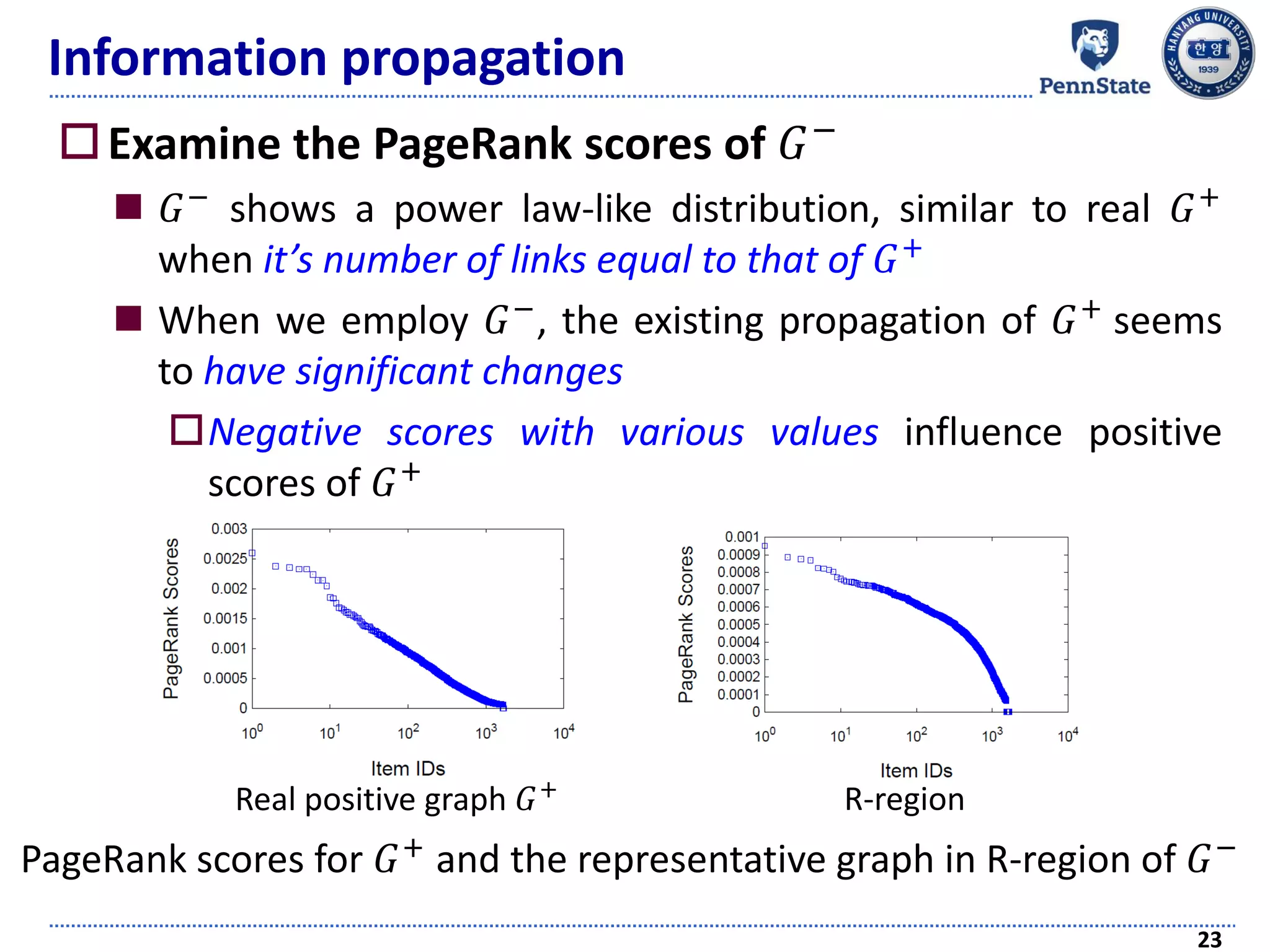
![Topological property
Graph shattering theory [Appel et al., SDM 09]
Introduces a “shattering point”
Connectivity of a graph becomes seriously collapsed
As links are continuously removed in a random way
ShatterPlot: visualizing the process of generating the
shattering point
17
ShatterPlot for positive graph 𝐺+
of MovieLens 100K](https://image.slidesharecdn.com/recommendersystemswithimplicitfeedbackchallengestechniquesandapplications-180410005822/75/Recommender-Systems-with-Implicit-Feedback-Challenges-Techniques-and-Applications-17-2048.jpg)
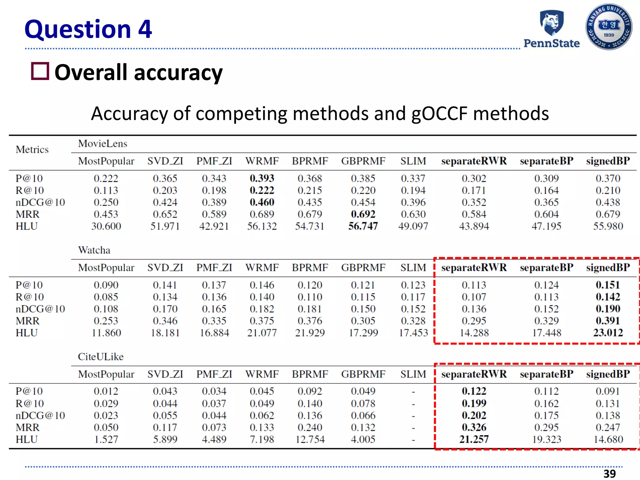
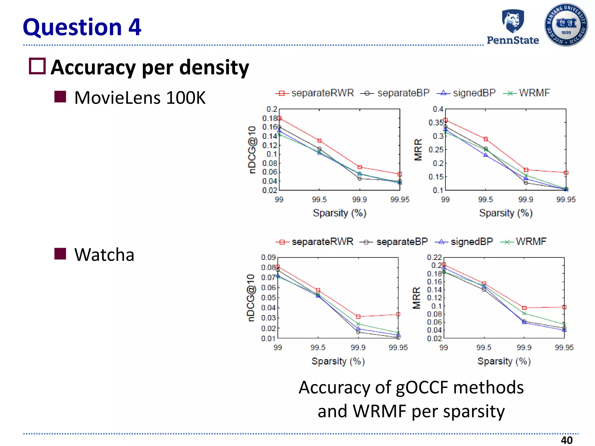
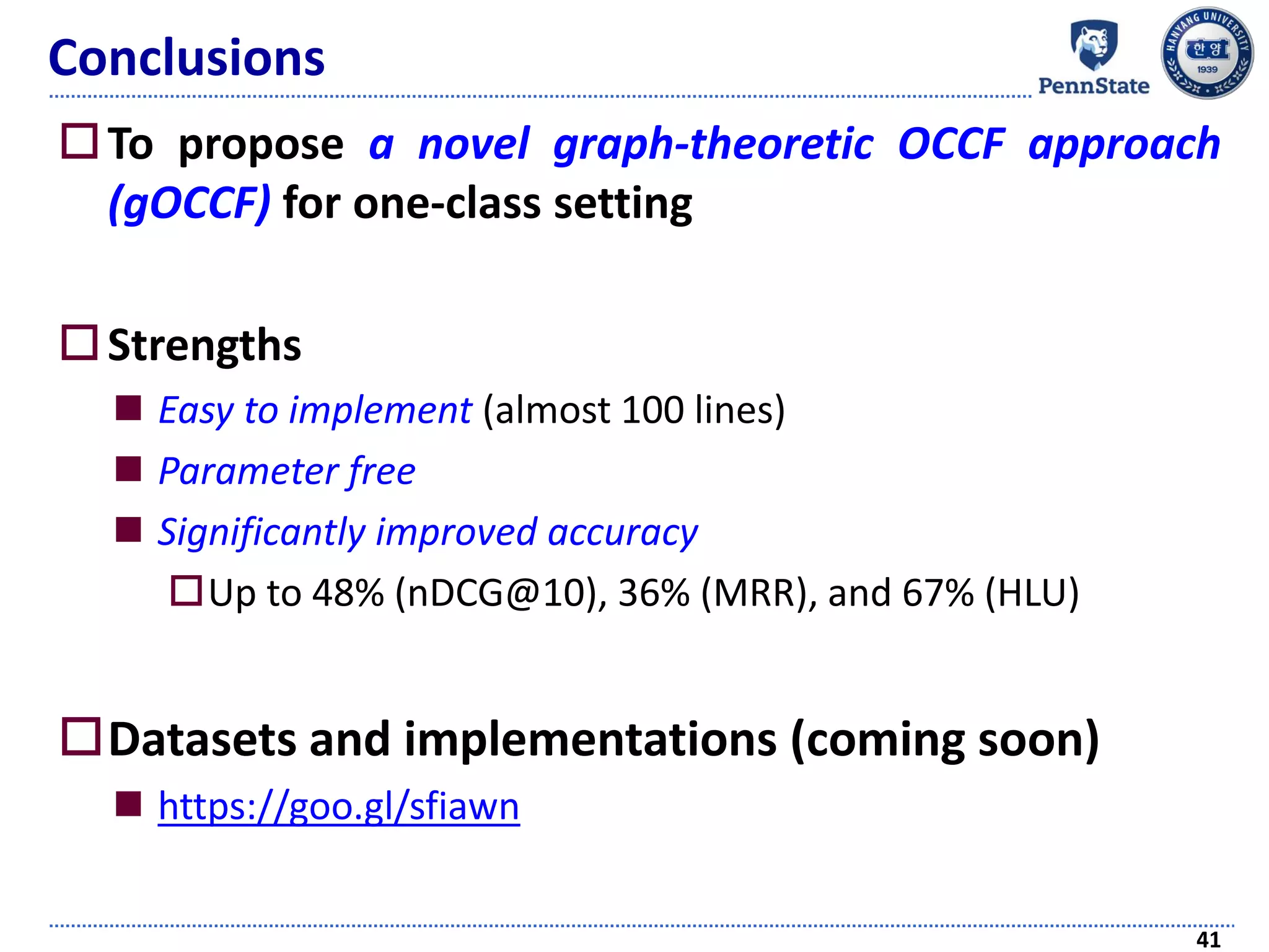

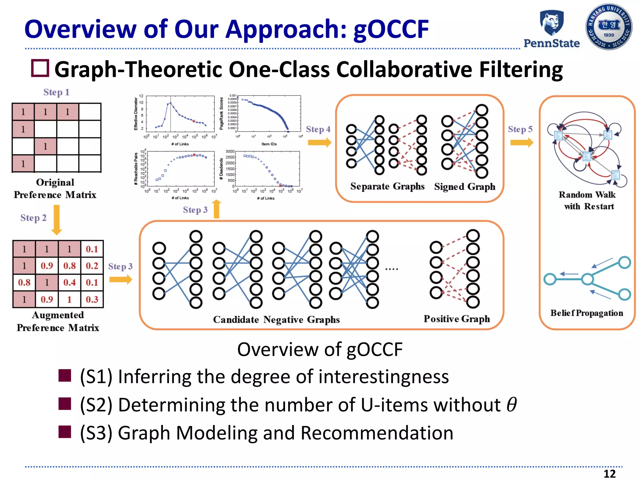
The document discusses challenges and techniques in recommender systems utilizing implicit feedback, particularly focusing on a novel approach called Graph-Theoretic One-Class Collaborative Filtering (GOCCF). It highlights the motivation behind GOCCF, which aims to better handle sparse datasets by inferring interestingness of items and modeling preferences using graph analysis. The document also outlines applications of this approach in job, paper, and TV show recommendations, showcasing its efficacy in improving recommendation accuracy.


![Coded Agents – with UiPath SDK + LangGraph [Virtual Hands-on Workshop]](https://cdn.slidesharecdn.com/ss_thumbnails/codedagentsdeck-251215155422-5497c599-thumbnail.jpg?width=640&height=640&fit=bounds)


